Ravenna : HEC Montréal, Institute of Applied Economics and CIRPÉE [email protected]
Thanks to Joshua Aizenman, Timothy Cogley, Oscar Jorda, Ken Kletzer, David Lopez-Salido, Carl Walsh and John Williams for useful comments and suggestions.
Cahier de recherche/Working Paper 14-09
How Central Banks Learn the True Model of the Economy
Federico Ravenna
Abstract:
Policy decisions affect economic outcomes, and the likelihood of observing a given state
of the world. We investigate how policy choices affect learning of the true model of the
economy when the policymaker’s model is mis-specified. We ask under what conditions
can the central bank learn the correct specification of the model describing the economy,
and what is the impact of exogenous shocks and of adopting an optimal monetary policy
on the speed of learning. Slow learning can occur simply because identifying the correct
model at standard confidence levels requires a long data sample. We show that neither
real-time learning by the policymaker or the private sector, nor the adoption of an
optimal policy, affect the speed of detection of model misspecification. Detection speed
depends instead on the relative volatility of supply and demand shocks.
Keywords: Learning, Optimal Policy, Model Misspecification
1
Introduction
The adoption of an optimal monetary policy requires knowledge of the model de-scribing the economy’s law of motion. Policy-makers look with caution at the pre-scriptions of optimal policy rules because they tend to be highly model-specific. The literature on optimal monetary policy under model uncertainty dates back at least to Brainard (1967), who showed how uncertainty in the models’ parameters would alter the optimal behaviour of the central bank. A growing literature has suggested several approaches to account for model uncertainty in policy design, including the use of robust control (Hansen and Sargent, 2003), policy rules robust to some form of model misspecification (Giannoni and Woodford, 2005) and model averaging methods (Brock et al., 2007, Cogley and Sargent, 2005, Cogley et al., 2011). These methodolo-gies aim at allowing policymakers to explicitly account for the likelihood of competing models to correctly describe the economy when choosing policy.
Nevertheless, policymakers may need to engage in model selection, and take a stand on what is the ’true’ model of the economy. For example, central banks need to produce forecasts of the economy, which constitute an important input in the policymaking process. Alternatively, policymakers may have a preference for policies which are independent of the continuous updating of model probabilities over time.
The central bank’s policy problem has two distinctive characteristics. First, policy choices depend on the available data and the understanding of the economy. At the same time, policy decisions affect economic outcomes, and the very data-generating process used as an input when estimating the economy’s model. Second, central banks do not base policy decisions on models that nest every possible specification. Therefore the problem of whether a central bank can learn the correct model often cannot be reduced to whether the true parameters can be estimated. The evolution of central bank behavior arises from switching to different (non-nested) models that can give better account of data observations (Sargent, 1999, suggest as an explanation of the move to a low-inflation environment in the 1980s the ’triumph of natural rate theories’).
In this paper we study the problem of a central bank which must identify the true model across competing alternatives while conducting policy according to its beliefs on the model of the economy. We assume the policymaker tries to detect the existence of misspecification in its believed model against a proposed alternative, while estimating in real time the deep parameters of the model needed to compute the optimal policy. We also allow for the private sector to learn over time the law of motion of the economy, as in Evans and Honkapohja (2003b). In this framework, we can assess whether the objective of selecting the correct model across competing
alternatives provides an incentive to deviate from the full-information optimal policy, as in Wieland (2000).
Our results show that a central bank using an optimal policy updated in real-time can detect the misspecification in its believed model as fast as a non-optimizing poli-cymaker setting policy using a given Taylor-type rule. Behaving optimally does not affect the likelihood that equilibrium outcomes are observed that reveal the model mis-specification to the policymaker. Moreover, real-time learning of the model pa-rameters by the policymaker or of the law of motion by the private sector does not affect the speed of misspecification detection. Crucially, our results depend on the relative volatility of supply and demand shocks. When supply shocks are sufficiently more volatile than demand shocks, detection of the model misspecification does not occur even after the central bank has accumulated a 25-year long sample of data.
In our analysis we focus on competing models for the inflation process within a new Keynesian business cycle framework. Our choice of competing models reflects a long-standing debate on the nature of inflation inertia - whether inflation is driven by inertial exogenous shocks, or by an endogenous inertial mechanism for price updating - which has proven up to date difficult to resolve using available data. We assume the central bank believes inflation is a completely forward-looking variable. Therefore, costless disinflations are possible, and persistence in inflation is driven by persistence in the inflation equation’s shock process. Goodfriend and King (2001) show this to be a plausible model of the US inflation behaviour. The true model embeds a substantial degree of inflation inertia, and an i.i.d. supply-side shock process, in the spirit of the Fuhrer and Moore (1995) model of US inflation dynamics. While both models imply long-run neutrality, they have sharply different implications on the speed of disinflation, the central bank’s mis-specified model calling for instantaneous disinflation, the true model requiring gradualism.
A large literature on real-time learning studies the stability of REE when the private sector updates the model’s estimate recursively, for a given policy rule (Evans and Honkapohja, 2003b). Evans and Honkapohja (2003a) and Dennis and Ravenna (2008) examine the case of a central bank estimating the model’s parameters in real time, and updating its estimate when formulating the optimal policy. Within the real-time learning framework, we examine the problem of a central bank which must also select across non-nested model alternatives. Cogley and Sargent (2005) and Cogley et al. (2011) are closer in spirit to our work, assuming that the central bank updates the probability assigned to alternative reference models when formulating policy. These contributions rely on model averaging in a Bayesian learning framework, thus the optimal policy is affected by the possibility of large losses in competing models, even if they have a very low probability of being correct. Our analysis focuses on
the econometric problem of distinguishing across model alternatives in a real-time learning environment. As in most of the learning literature, we assume a boundedly rational policymaker does not account for uncertainty in the parameters estimate when implementing policy, or for the learning process of the private sector.
2
Can the Central Bank Learn the true model? An Easy
Example
This section uses a simple form of model mis-specification to illustrate the issues arising when the central bank is at the same time trying to learn the true structure of the economy and setting policy optimally.
2.1
Irrelevant mis-specifications
The economy is described by a log-linear, two-equations New-Keynesian model (widely adopted in the optimal monetary policy literature, see Clarida, Gali, and Gertler, 1999). The central bank believes the inflation equation includes an unobservable,
exogenous cost push shock when no such shock appears in true model:
Central bank = +1+ + (1)
mis-specified model = +1− (− +1) + (2)
= −1+ ; = −1+
where is inflation, is the output gap, is the nominal interest rate, is an i.i.d.
random variable. Given a loss function ( ∞) = P∞=0
h
2++ 2+i the
optimal time-consistent policy first order conditions are given by eqs. (1), (2) and:
= −
(3)
Conditional on the optimal policy, the central bank expects to observe the follow-ing equilibrium law of motion:
= (4)
= − (5)
= 1
2+ (1 − )
This set of equations describes the central bank’s Perceived Law of Motion ( ) as defined in Evans and Honkapohja (2003a). The optimal policy can be implemented
through an instrument rule that does not depend explicitly on the unobservable shock : = ∙ 1 + (1 − ) −1 ¸ +1+ −1 (6)
The true model of the economy is given by:
True Model = +1+
= +1− (− +1) +
= −1+
What is the Rational Expectation Equilibrium () of the economy? It is straightforward to show that the true model and the policy rule (6) lead to the :
= 0
= 0
This is the same equilibrium that we would observe if the central bank
imple-mented the optimal policy conditional on the true model: = −11. For this kind
of model mis-specification, two results emerge. First, the mis-specification does not
lead to any welfare loss: the policy rule (6) can sustain the optimal 2 Second,
the central bank would never be able to learn the mis-specification, since both
and have zero variance in the . The very policy chosen by the central bank
prevents econometric estimation and testing of the model in eqs. (1), (2). In other words, the fact that the optimal equilibrium can be attained does not imply that the central bank knows the true model.
If the private sector is trying to learn the law of motion of the economy, will the
be attained? It can be shown that the optimal , = = 0 (the True
Law of Motion, or ) can be learnt - the is E-stable. Let = [ ]0. The
private sector needs to form expectations of +1 +1 Assume the private sector
Perceived Law of Motion ( ) takes the form:
+1= 21
where is not the mathematical expectation of a variable, but the expectation
conditional on current knowledge of the reduced form model of the economy. In
1
It is well known that this rule leads to indeterminacy (Woodford, 2003). This point is not crucial for the issue at hand, and is illustrated in the following section.
2This result extends to some other model mis-specifications, but is not true in general. For
example, with habit-persistent preferences the true output-gap equation is = (1 − )+1+
−1− (− +1) + . The mis-specified output-gap dynamics (2) would not have any impact
this model, the is E-stable if both rows of the vector converge to 0 as the private sector updates its estimate of (under some regularity conditions). Since the true law of motion in this example corresponds to the optimal , learnability of the would imply learnability of the optimal policy rule by the central bank
- although not learnability of the true model3.
2.2
Easily learnable mis-specifications
Contrary to the previous example, most model mis-specifications cause a welfare loss. Assume that the central bank is not aware of the existence of cost-push disturbances to the inflation equation, whereas they do exist in the true model of the economy:
Central Bank Model True Model
= +1+ = +1+ +
= +1− (− +1) + = +1− (− +1) +
= −1+ = −1+ ; = −1+
The time-consistent optimal policy first order conditions are given by the central bank’s model and:
= −
(7)
The optimal policy can be implemented using the policy rule = −1. Since
this rule would lead to indeterminacy and E-instability, we assume the central bank implements the policy:
= +1+ −1
1
Model mis-specification leads to a welfare loss Conditional on the central
bank policy, the - or true law of motion ( ) - is:
= 0
= 0
0 = ; 0 = (1 − )−1
= (1 − ) − [(1 − ) + (1 + )]
3
While this conclusion would require a formal proof and a complete specification of the Central Bank’s learning process, an even stronger result is true in this example: learnability of the implies learnability of the optimal , regardless of whether the Central Bank is updating its model, provided the parameter is known.
But the model mis-specification implies a loss in the economy’s welfare: the under the true optimal policy is different, and is given by eqs. (4), (5). Notice that the is E-stable, but inefficient.
Mis-specification detectability Can the central bank realize it is using a
mis-specified model? The monetary authority perceived law of motion ( ) is given by:
= 0
= 0
whereas the actual law of motion ( ) has been shown to be:
= 0
= 0
Therefore, by comparing the economy’s dynamics to the the central bank can easily realize its model suffers from specification. We will say that the mis-specification is ’detectable’ if the allows econometric identification of the model - if differences between the believed model and any alternative model lead to testable restrictions in the law of motion.
The speed of learning In this example, all that the central bank needs to detect
the mis-specification is one observation. In general, this is not the case: learning takes time, many observations may be needed to be able to reject a false model. The speed of learning is affected by the policy adopted: although in this model any policy
would lead to an instantaneous learning, since the shock is observable. The speed
of learning is also a function of the random disturbances: even in this easy example,
until a shock occurs, the central bank would have no reason to reject the model,
since conditional on the and the are identical.
The usefulness of Robust Optimal Explicit rules Giannoni and Woodford
(2005) discuss policy rules (Robust Optimal Explicit, or ROE rules) which are invari-ant to the random disturbances affecting the economy. Essentially, they suggest using as policy rule the first order conditions of the optimal policy problem which do not involve random shocks. In the two previous example, this corresponds to assuming
the monetary authority can use as an instrument. In fact, the first order
condi-tions (3) and (7) are identical, since the only differences in the two models is in the disturbances. It is true that using the ROE rule would allow the optimal to be
achieved in both examples. Unfortunately, this is not the case for more sophisticated mis-specifications. To illustrate this point, in the following section we will always use the ROE rule.
Robustness to parameter uncertainty In this example, the monetary authority
could easily guard itself from mis-specification by adopting the inflation equation specification:
= +1+ + (8)
and using an optimal policy rule robust to uncertainty in the parameter . While this is a wise strategy, it will only work if the alternative (true) model is a restricted version of the estimated equation (8) - if the estimated model the alternative. As we show in the following section, often even very straightforward model alterna-tives can be non-nested. This implies that robustness to parameter uncertainty is of limited help when addressing the issue of model mis-specification in formulating the optimal policy
3
The model
3.1
The true model
The model that we analyze is a sticky-price New Keynesian model widely used in the monetary policy literature. Households are assumed to consume a Dixit-Stiglitz aggregate of the goods firms produce, choosing consumption, leisure, and their
hold-ings of real money balances to maximize utility. Household consumption behavior
is governed by
= −1+ (1 − )+1+ (− +1) + (9)
where , and are the consumption gap, inflation, and the nominal interest rate,
respectively. The lagged consumption term in equation (9) is motivated by external habit formation. In equation (9), is the intertemporal elasticity of substitution,
is a function of the degree of habit formation and is a consumption preference
shock.4 In the special case where there is no habit formation, = 0, equation (9)
collapses to the standard Euler equation for consumption with time-separable utility. The economy’s resource constraint equates consumption to output, which implies
that equation (1) can be expressed in terms of either consumption or output. In
what follows we use equation (9) to describe the behavior of the output gap, which
we denote by .
4Formal derivations of equation (9) can be found in McCallum and Nelson (1999) and Amato and
On the supply side, we assume each period a fixed share of firms is able to
re-optimize their price. However, within this share, a fixed proportion of firms
un-dertakes the standard Calvo (1983) re-optimization while the remaining firms adjust their price to the time − 1 price chosen by the optimizing firms adjusted for the lagged aggregate inflation rate. Galí and Gertler (1999) show that this model implies the behavior of inflation can be summarized by the Phillips curve equation
= (1 − ) +1+ −1+ + (10)
where denotes real marginal costs and is a supply shock. In equation (10),
is the discount factor while and are composite parameters that depend on
the share of Calvo-pricing firms and on the share of indexing firms. While the
underlying theory implies that real marginal costs should be the driving variable in the Phillips curve, we follow Clarida, Galí, and Gertler (1999) and substitute the
output gap for real marginal costs . 5 We assume that the supply shock and
the consumption preference shock are independent, white noise processes, with finite absolute moments. We further assume that the parameters in equations (9) and (10) satisfy 0 ≤ ≤ 1 0 1, 0, and 0.
While equations (9) and (10) are reasonably simple, and are intended to serve only as a stylized description of the economy, they encompass several widely studied
macroeconomic models. As noted earlier, when = 0, equation (9) collapses to
the standard (log-linearized) time-separable consumption Euler equation. Similarly, when = 1 equation (10) corresponds to a backward-looking accelerationist Phillips curve (Ball, 1999) and when = 0 equation (10) simplifies to the traditional Calvo-pricing specification. Further, if = 0 and = 1, then equation (10) is equivalent to the costly-price-adjustment specification of Rotemberg and Woodford (1982). Inter-mediate values of accommodate Phillips curves with complete inflation indexation (Christiano, Eichenbaum, and Evans, 2005) and partial inflation indexation (Smets and Wouters, 2003).
3.2
Monetary policy
We assume that monetary policy is set under discretion and the central bank chooses
the nominal interest rate, , to minimize the loss function
( ∞) = ∞ X =0 h2++ 2++ (∆+)2 i (11)
5In the absence of habit formation, it is easily shown that real marginal costs are directly
propor-tional to the gap. See Amato and Laubach (2004) or Dennis (2004) for derivations of the relationship between the gap and real marginal costs in the presence of habit formation.
subject to the behavior of households and firms, as summarized by equations (9) and (10). This loss function postulates that the central bank aims to stabilize inflation
and the output gap avoiding large changes in the nominal interest rate. With the
weight on inflation stabilization normalized to one, the relative weight on output stabilization is ≥ 0 and the relative weight on interest rate smoothing is ≥ 0.
To solve the model we use the procedure developed in Dennis (2007) to solve for the Euler equation, or targeting rule, associated with the optimal discretionary policy. A key feature of this targeting rule is that it is expressed in terms of endogenous
variables and excludes the shocks, and . As a consequence, it is robust, to
mis-specification of the shocks process. In addition to the Euler equation for the optimal discretionary policy, the solution algorithm yields decision rules for inflation, the output gap, and the nominal interest rate that take the form
z= Az−1+ Bv (12) where z= £ ¤0 and v= £ ¤0 .
3.3
Model parameterization
To simulate the model we require benchmark values for each of the parameters in the model. We set equal to 050 and equal to 030. With these values, consumption and inflation are persistent, but consumption smoothing and the forward looking
nature of price setting remain prominent. The household’s discount factor, , is
set to 099. Two parameters that are central in our analysis are and . In our
simulations = −015 and = 020. In our benchmark parameterization for the central bank preferences we set = 100 and = 05. Finally, we set the standard deviations of the demand and supply shocks equal to 15.
3.4
The Central Bank Model
The central bank believes that the dynamics for inflation and the output gap are described by
= −1+ (1 − )+1− (− +1) + (13)
= +1+ + (14)
= −1+
Thus the central bank believes that the economy is impacted by serially corre-lated supply shocks whereas in fact its model mis-specifies the economy’s inflation
and output dynamics. The perceived supply shock, , truly represents model
mis-specification and evolves according to
= −+1+ −1+ (15)
Both the true and central bank’s specification imply and display autocorrelation
under the (respective) optimal policy. But they have radically different implications for the way the central bank should move its instrument in response to shocks, for the cost of moving to a lower steady-state inflation level, and for the optimal way to achieve it (Clarida, Gali and Gertler, 1999, offer a detailed discussion). The central bank believes disinflation can be achieved without any cost, while a monetary authority which knows the true model and has a quadratic loss function in inflation would find optimal a gradual inflation reduction.
3.5
Central Bank Learning
The central bank formulates the optimal policy conditional on eqs. (13), (14) and on the real-time estimate of the unknown parameters Since the central bank puts
a positive weight on and ∆in the objective function, the set of state variables
under the mis-specified model is the same as in true model: −1 −1 −1. To
have a meaningful mis-specification problem in the estimation, we must assume that
at least the shock is unobservable to the policy maker. This assumption still leaves
the central bank a choice of three instruments to use in the GIV estimator.
The Robust Optimal Explicit rule involves and lagged values of the nomi-nal interest rate, and therefore gives an instrument rule independent of the exogenous shock process for the cost-push shock. This also means that estimates of the coeffi-cient do not need to enter the formulation of the optimal policy.
Replacing expected values with realizations for estimation purposes, equation (13) becomes
= − (− +1) + − (1 − )+1+ +1 (16)
≡ − −1− (1 − )+1
where +1−+1= +1and +1−+1= +1 Similarly, with and assumed
to be known, the Phillips curve can be expressed as
− +1= + (17)
Once expected future inflation is replaced with observed inflation, introducing an expectation error to the dependant variable, we obtain:
= + − +1 (18)
Since is an AR(1) process, lagged values of all the variables will be correlated with
the error term, and will not satisfy the necessary condition for instrument validity. We assume the central bank uses the Cochrane-Orcutt transform:
(1 − ) = (1 − )+ (1 − )(− +1)
= −1+ − −1+ ( +e+1) (19)
where both and e+1 are i.i.d. shocks and is the lag operator. Efficient
estimation would require the use of a NLIV estimator (see Fair, 1970), but we assume the central bank estimates equation (19) without imposing the non-linear parameter
restriction. −1 can serve as instrument for while −1 −1 are valid instruments
for the remaining endogenous regressors. Note that while needs to be estimated, it does not appear in the optimal policy rule.
3.6
Private Sector Learning
We assume private agents estimate the economy’s equilibrium relationships and use these estimated relationships to form expectations of future output and inflation. The private sector is assumed to know the structure of the economy and have an
information set given by = { −1}.
Rewrite the structural model in matrix form:
0= 1−1+ 2+1+ 3 (20)
The REE takes the form:
z= Az−1+ Bv (21)
Substituting from the REE equations +1= into the structural equations
system, gives the matrix quadratic equations:
= (0− 2)−11 (22)
= (0− 2)−13
which can be solved for the matrices and
Assume that the private sector forms expectations ∗+1 according to the
Per-ceived Law of Motion (PLM ) and the estimated matrices ∗ ∗ :
Then:
∗+1= ∗+ ∗+1 (24)
Substituting eq. (24) in the structural model gives:
0= 1−1+ 2∗+1+ 3
The reduced-form dynamics of the economy, or Actual Law of Motion (ALM ), is then:
z= Az−1+ Bv (25)
where
= (0− 2∗)−11 (26)
= (0− 2∗)−13
Comparing eqs. (22) and (26) it is clear that 6= unless we are in the REE.
Moreover, 6= ∗ therefore as more observations are generated the private
sector estimates of will change. Finally, when the central bank’s model is mis-specified, the REE is different from the optimal REE.
4
How Central Banks Learn: Competing Reference
Mod-els
4.1
Evaluating reference models
This section asks whether the economy may eventually attain the optimal REE from any suboptimal one that has been reached because of the central bank model mis-specification. Can the central bank realize the model mis-specification by estimating competing models, and selecting among them? If the competing models have testable implications, we expect the central bank will be able to detect which one is the true model, since this will be the one with the highest probability of having generated the data observed. In the following we examine the model mis-specification detectability, and the impact on the speed of learning of the policy rule chosen by the central bank and of the relative shocks variance.
4.2
Optimal monetary policy and non-nested models
Whenever model uncertainty cannot be described in terms of parameter uncertainty the fact that the competing models are non-nested complicates the central bank learning problem at two separate stages - in devising the optimal monetary policy, and in estimating the correct model. In general, optimal policy rules robust to parameter
uncertainty and robust optimal explicit rules are of no help to deal with this kind of model uncertainty. Recall that: Central Bank = +1+ + (27) mis-specified model = −1+ (1 − )+1− (− +1) + (28) = −1+ (29) True model = (1 − ) +1+ −1+ + (30) = −1+ (1 − )+1− (− +1) + (31)
If the monetary authority considered the true model as a possible alternative, how would it alter its current policy-making?
First, the central bank faces an econometric problem. Consider the case when all parameters are unknown. It is useful to build an encompassing model of the inflation equation to be used for estimation purposes:
=
1
1 + (1 − ){(1 − )+1+ ( + )−1− −2+ − −1}+
0 (32)
Eq. (32) is obtained from a model given by eqs. (29), (30) and (31). The variable
+1 is replaced with the realized value +1 and the Cochrane-Orcutt transform
is applied, so that the term 0 is a linear function of i.i.d. Gaussian variables (the
shock
and a forecast error). The vector of parameters values b can be estimated
using a non-linear instrumental variables estimator (provided enough instruments are available). Under the hypothesis = 0 we obtain the central bank model’s inflation equation needed for estimation of the unknown parameters:
=
1
1 + {+1+ −1+ − −1} +
0
(33)
while under the hypothesis = 0 we obtain the true model inflation equation :
= (1 − )+1+ −1+ + 0 (34)
These model alternatives are non-nested. The parameter space of each alternative
is a subset of the parameter space of the unrestricted model (32): b = ( ), but
neither model can be obtained as a restriction on the other.
Estimation of equation (32) will likely return biased estimates since we are
includ-ing the irrelevant regressor −2 whereas under either the central bank or the true
necessarily true that adding an irrelevant regressor does not affect the unbiasedness of the estimator.
Second, and independently from how the estimation problem is dealt with, there is no compelling reason for the central bank to use an encompassing model to formulate the optimal monetary policy. The optimizing policymaker knows with certainty that this model is incorrectly specified. When models are non-nested it is clearly always possible to build a new model encompassing all alternative theories. In our case, it would be given by:
Encompassing = (1 − ) +1+ −1+ +
model = −1+ (1 − )+1− (− +1) +
= −1+
But this model has zero probability of being correct, and it is difficult to argue that it should be the basis for formulating an optimal policy. Effectively, endowing the policymaker with the information that the encompassing model is incorrect trans-forms the central bank problem from one of finding the correct parameters to one of finding the correct theory. Therefore, rules robust to parameter uncertainty built as in Brainard (1967) that use the encompassing model are of no help.
The challenge raised by non-nested alternatives becomes clear when we look at a case where competing models are nested. Consider the estimation problem faced by a central bank contemplating the choice between eq. (27) and (30). We now endow the central bank with knowledge of the fact that supply shocks are white noise. In this case the central bank could estimate eq. (34) and use eq. (30) in formulating policy. Eq. (30) nests the central bank model where = 0 Over time estimates of would converge to the true value, so the problem faced by the central bank becomes simply one of parameter uncertainty in one of the coefficients in the inflation equation. The central bank model, whatever the current estimate of will be the one with the highest probability of being correct conditional on the data available.
It is worth noting that, within the mis-specification we examine, using a Robust Optimal Explicit rule would offer the central bank the chance to effectively nest the alternative models in the optimization problem. Since the ROE rule is independent of the central bank can use the true model when optimizing - the shock processes equations do not enter the first order condition implementing the optimal policy. The fact that the estimable inflation equations (33) and (34) are non-nested is irrelevant for the optimization problem. This result is by no means general. For example, eq. (30) could easily be only an encompassing model, with the two alternatives characterized by = 0 and = 1 Then the problem of choosing the true model cannot be reduced anymore to parameter uncertainty, even adopting a ROE rule.
Many of the policy-making paradigm shifts which happened in the last decades involved choosing among non-nested alternatives. In the following we assume the central bank will abandon its current model and adopt the alternative one when the current model can be rejected at a given level of statistical significance.
If the central bank wished to take into account different models’ likelihood of being correct, it would be appropriate to use a Bayesian setup, as in Cogley and Sargent (2005), where competing models are assigned different, time-varying weights in the policymaker optimization problem. In this framework though the weight of any model on the shaping of policy can be different from the likelihood a model has of being correct, since each model enters into the calculation of expected discounted welfare in the policymaker’s optimization. Therefore a model can be learnt quickly, but still have a small impact on policy. We instead assume that once a model can be rejected, its weight drops to zero. Slow learning can simply be the outcome of the slow convergence of the estimator, coupled with the central bank and private sector affecting the data generating process.
4.3
Detectability with reduced-form estimation
The central bank model, eqs. (27), (28) and (29), and the alternative model, eqs. (30) and (31), have reduced form representation:
= [ ]−1+ [ ] (35)
where = [ ]0 = [ ]0 = [ ]0. The optimal monetary
policy conditional on the central bank model implies that −1 is not a state variable
in the REE. On the contrary, if the alternative model is true all variables are state variables. If all variables and shocks were observable, the central bank would only need one observation to discriminate between the two models. Since the vector is unobservable, the policy-maker must rely on statistical testing to determine whether
the restriction = 0 is validated by the data.
How long will it take to discriminate between the alternative models? We ran 500 simulations to determine the average learning time, assuming that the central bank has available an initial sample of twenty observations (five years at a quarterly
frequency), generated by the true model conditional on the rule = 15+05 The
policy maker estimates the model parameters and updates the optimal policy, and in every period also estimates the VAR reduced form (35) to test the restriction
on the vector The likelihood ratio test compares the hypotheses:
0 : = 0
through the likelihood ratio statistics Λ = (ln | | − ln |∗|) is the residual
covariance matrix based on the restricted (true) model, whereas ∗ is the
corre-sponding statistic for the unrestricted model.
We evaluate the speed of detection using two different measures. First, we build the average p-value of the statistic Λ across the different simulations, at each period Since there are 20 initial observations, the sample size at time is +20 To provide a measure of how the data volatility affects speed of detection in individual samples, we also build an average detection time statistic, reporting the average of the number of observations necessary in each simulation run to obtain four consecutive rejections of the null hypothesis at 5% confidence - we assume after a full year the central bank can reject its model, it switches to the alternative one.
Figure 1 shows the average p-value at time . Mis-specification detection is quite slow - it takes over 15 years of data for the average p-value of the null hypothesis to fall in the 5% rejection region. The test average speed of detection is 34 quarters.
0 10 20 3 0 4 0 5 0 6 0 7 0 8 0 90 1 0 0 0 5 1 0 1 5 2 0 2 5 3 0 3 5 F i g . 1 0 : R e s t r ic t e d m o d e l V AR e s tim a t e s : A v er a g e p - va l ue at tim e t fo r H 0 C e n t r al B a nk lea r n in g N o le ar n in g t
Figure 1: Restricted model VAR estimates: average p-value for 0 at time
Does the central bank real-time learning of the model parameters slow the de-tection process? Not in a significant way. Using the same random draw, we ran the simulation giving full knowledge to the central bank of the parameter values. The av-erage p-value is very close to the previous case at every horizon, and the test avav-erage speed of detection rises to 36 quarters.
Reduced-form testing cannot be used if the private sector is learning too. In this case, rejection of the null hypothesis would not imply a model mis-specification: it could also originate from the private sector forecasting function not having converged
to the REE. In principle it is always possible for the central bank to estimate the
private sector forecasting model, build the predicted [ ] vector using the
opti-mal policy rule and the private sector expectations, and test it as the null hypothesis against the estimated actual law of motion. But this implies that the central bank has full knowledge of the private sector forecasting model.
In the same fashion, testing the restriction = 0 is not a valid test of the central
bank model if the policy rule is given by a Taylor rule, such as = 15+ 05
Then the vector [ ] would have no zero elements conditional on any of the two
alternative models.
4.4
Detectability with structural estimation
Structural estimation allows us to examine the impact of a wider range of parameters on the learning speed. As in the previous section, the central bank in every period up-dates the estimates for of the current (mis-specified) model (27) and re-optimizes conditional on the new information. The private sector updates its estimates of the law of motion, and generates expectations of future variables. The policymaker is also endowed with the alternative (true) model (30), and in every period tests the hypothesis that the current model is correct.
There is a number of ways in which the two models can be statistically compared. First, the policymaker can use any of a long list of test for non-nested models (see Greene, 2003). Most of these tests though have been devised for linear models and in the context of OLS estimation (see Godfrey, 1983 for an extension of the Cox, 1961, test to the IV estimator)
We examine an easier testing strategy. The central bank can estimate eq. (33). While this equation’s coefficient vector does not nest the alternative eq. (34) coef-ficient vector, its reduced-form, linear unrestricted coefficient vector does nest the alternative. The central bank can distinguish the two models by testing whether
the coefficient on −1 is significantly different from zero. This methodology has the
advantage that we do not need to assume knowledge of or and do not involve tests of these coefficients. On the other hand, the central bank would be using for models selection an equation different from the one used for model estimation.
In our simulations we rearranged equation (33) for estimation purposes6, so that
6
This specification is also used in Linde (2005) when testing the New Keynesian inflation equation. We found the test performs better when compared to the results from estimating eq. (33), but the results are qualitatively unaltered.
the two alternative equations are: +1 = 1 [−−1− + −1+ (1 + )] + +1 +1 = 1 (1 − )[−−1− + ] + +1
and is an i.i.d. Gaussian random variable. We assume the policy maker runs
two Wald test on the estimated equation.
+1= + 1−1+ 2+ 3−1+ 4+ +1 (36)
The first test compares the hypotheses:
0 : 3= 0
1 : 36= 0
If 0 cannot be rejected, doubt is cast on the central bank’s model. Since the
acceptance region for 0 can be very large, we assume the mis-specification detection
occurs when the policy maker cannot reject 0 and at the same time can reject 2
in the test:
2 : 3 =
3 : 3 6=
The parameter is set equal to 05 - a very large value, which will bias the test
towards detection, given 4= the true value of is 02 and 1
To build the test statistics, we need an estimate of the asymptotic variance of 3
Since the regressors are correlated with the error term, we would need to use an IV estimator. The need to estimate four regression coefficients (beyond the constant)
lead us to the choice of four instruments: −1 −1 −1 −2 Conditional on the
true model, only the first three are valid instruments, whereas conditional on the
central bank model the only valid instruments are −1 and −1 Given that in the
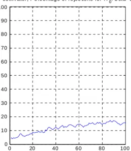
simulations both the private sector and the central bank are updating their estimates in real time, we can expect our list of instruments will be appropriate, although not asymptotically in the REE. To check the power of the test, we ran 500 simulations assuming all agents have full information, and no learning takes place. It takes several hundred observation for the coefficients to converge to the population values. The large variance of the estimates makes the Wald statistics a very weak test in detecting model mis-specification, unless the sample is in the thousands of observation. Figure 2 (panels A and B) shows the percentage of rejections of the two null hypotheses
slowly with the sample size, and after a 25 year-long span still amounts to less than 20% of the simulations. 0 20 40 60 80 10 0 0 0.2 0.4 0.6 0.8 1 1.2 1.4
IV e stim at or, Pe rc ent ag e o f re jec tio ns for H
0: b et a=0 0 20 40 60 80 100 0 10 20 30 40 50 60 70 80 90 100
IV es tim ator, P e rc entage of re jec tions for H
0: b et a= 0 .5 0 20 40 60 80 10 0 0 2 4 6 8 10 12 14 16 18 20
O LS es tim ato r, P erce nta ge of rejec tion s f or H
0: bet a= 0 s am ple s iz e 0 20 40 60 80 100 30 40 50 60 70 80 90 100
O LS es tim ato r, Pe rce nta ge of rejec tion s f or H
0: beta= 0.5
sa m ple siz e
Fig. 11
Figure 2: Structural model: percentage of rejections of the two null hypotheses
If the central bank were to rely on asymptotic theory for testing the IV estimates, it would never be able to detect the model mis-specification except after several decades. Learning cannot happen.
There is obviously an advantage in terms of estimator asymptotic variance in using an OLS rather than an IV estimator. On the other hand, the OLS estimate of the vector is inconsistent, and its asymptotic variance does not converge to zero, if correlation between the regressor and the error term exists. Whether this correlation is such to make the IV estimator superior to the OLS estimator in our testing environment is an empirical issue that we investigated. The very large variance of the IV estimator implies that an Hausman test could not reject the null hypothesis that the OLS estimator is consistent. Running 500 simulations (using the same random draws as in the previous sections) we ascertained that the OLS estimate of
3 is consistent. Figure 2 (panels C and D) shows the percentage of rejections of the
two null hypothesis using the OLS estimator, in the case when no agent is learning7.
The performance of the OLS estimator Wald test is clearly superior, and the sample size for which the test is asymptotically valid is an order of magnitude lower than in the IV estimator case.
Structural OLS estimation allows us to examine the impact of the learning en-vironment and of many other variables that may affect the learning speed, to which the estimated equation is invariant.
4.4.1 The Impact of Learning
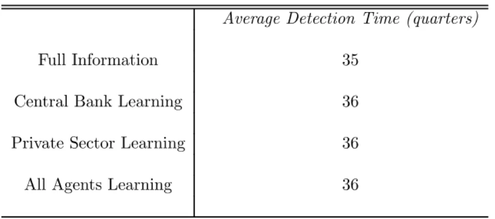
Mis-specification detectability and speed of learning Table 1 reports the
average detection time for the misspecification in the central bank’s model, measured
using the average number of quarters after which 0 cannot be rejected and 2 is
rejected at 10% significance level for four consecutive samples.
7
Therefore, the asymptotic variance of is calculated as 2[0]−1. The estimated asymp-totic variance for the IV estimator is given by 2[0(0)−1(0)]−1where is the matrix of regressors, the matrix of instruments, 2 is a consistent estimate of the error variance.
Table 1: Model selection and the impact of learning Average Detection Time (quarters)
Full Information 35
Central Bank Learning 36
Private Sector Learning 36
All Agents Learning 36
Note: Average Detection Time for2 using Wald test, OLS estimator, equation
(36). Average number of quarters after which0 cannot be rejected and2 is
rejected at10%confidence for four consecutive observations. The total sample
size is equal to the detection time plus the initial 20 observations. Initial obser-vations are generated using a Taylor rule. All simulations use the same random
draws from a normal distribution. The volatility of the shocks is2
= 2 = 15
Central Bank real-time learning Does the real-time learning behaviour of the
central bank impact the speed of detection? Interestingly, very little. The first line of Table 1 shows that in the full information case the learning speed is about the same as in the case when the central bank is estimating the values of and in real time.
Private sector learning The simulations show that the private sector learns very
fast how to use the model’s reduced form to generate its forecast. When the private sector is learning - either with or without the central bank also estimating the model’s parameters - mis-specification detection happens at about the same speed as in the full information case. This result indicates that (in the context of our model) the welfare loss due to the optimal monetary policy ignoring private sector learning is likely to become negligible very fast.
4.4.2 Shocks volatility and detectability
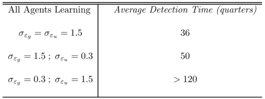
The speed of model misspecification detection is heavily impacted by the shocks
realization. Table 2 shows that relative to our baseline case, where 2 = 2 = 15
40% The learning speed changes dramatically if the volatility of demand shocks
decreases, so that 22 = 15. In this case, learning has not happened even after
30 years.
Table 2: Model selection and the impact of shocks
All Agents Learning Average Detection Time (quarters)
= = 15 36
= 15 ; = 03 50
= 03 ; = 15 120
Note: Average Detection Time is the average number of quarters after which
0 cannot be rejected and 2 is rejected at 10% significance level for four
consecutive samples, computed over 500 simulations.
4.4.3 Does optimal monetary policy slow learning?
Wieland (2000) argues that a central bank weighing the advantages of learning fast against the advantages of using an optimal policy conditional on partial information may find desirable to generate spurts of large volatility in the economy to speed up the learning process. Within our framework, using an optimal policy does not penalize significantly the learning speed of the policy-maker. Table 3 shows the average detection time for the optimizing policymaker, compared to the one achieved
by a policymaker using a Taylor rule = 15+ 05 While there will be
non-optimizing policy rule that can slow down learning, using an optimal policy does not put the policy-maker at a clear disadvantage in the context of the New-Keynesian model.
Table 3: Model selection and the impact of policy
Average Detection Time (quarters)
All Agents Learning - optimal policy 36
Private sector Learning - Taylor rule 38
Full Information - Taylor rule 36
Note: Under the Taylor rule case the central bank uses the policy =
15+ 05
5
Conclusions
This paper uses a New Keynesian model of the business cycle to investigate how policy choices affect the policymakers’ ability to learn the structure of the economy. We examine the probability with which an optimizing central bank will detect that it is using a mis-specified model. We investigate numerically under what conditions the true model can be learnt, focusing on how the random innovations and the choice of policy affect the speed at which learning is achieved.
Our results show that a central bank attempting to stabilize the economy using an optimal policy while trying to identify the true model learns at about the same speed as a non-optimizing policymaker - for example, one that sets policy using a forward-looking Taylor-type rule. Behaving optimally does not affect the likelihood that equilibrium outcomes are observed that reveal the model mis-specification to the policymaker. Learning by either the central bank or the private sector does not significantly affect the average length of the data sample a central bank needs to detect a misspecification in its model of the economy. While there may exist an incentive for experimentation, using the boundedly-rational optimal policy does not put the policy-maker at a clear disadvantage in the context of the our model. This result crucially depends on the relative volatility of the supply and demand shocks. When the supply shock volatility is five times as large as the demand shock, model misspecification can go undetected for over 30 years.This finding suggests that switching between competing models of the economy is potentially related to large swings in the volatility of the process driving the business cycle.
References
[1] Aoki, K. and Nikolov, K., (2004), ”Rule-based Monetary Policy under Central Bank Learning”, in Clarida, R., Frankel, J. and Giavazzi, F., eds., International Seminar in Macroeconomics Conference Proceedings, NBER: Boston.
[2] Amato, J., and T. Laubach, (2004), “Implications of Habit Formation for Opti-mal Monetary Policy,” Journal of Monetary Economics, 51, pp305—325.
[3] Ball, L., (1991), “The Genesis of Inflation and the Costs of Disinflation,” Journal of Money, Credit and Banking, 23, 3, pp439—451.
[4] Ball, L., (1999), “Efficient Rules for Monetary Policy,” International Finance, 2, pp63-83.
[5] Brainard, W., (1967), “Uncertainty and the Effectiveness of Policy,” American Economic Review, 57, pp411-425.
[6] Brock, W., Durlauf, S. and West, K., (2007), "Model uncertainty and policy evaluation: some theory and empirics", Journal of Econometrics, 136, 629-664. [7] Bullard, J., and K. Mitra, (2002), “Learning about Monetary Policy Rules,”
Journal of Monetary Economics, 49, 6, pp1105-1129.
[8] Calvo, G., (1983), “Staggered Contracts in a Utility-Maximising Framework,” Journal of Monetary Economics, 12, pp383-398.
[9] Christiano, L., Eichenbaum, M., and C. Evans, (2005), “Nominal Rigidities and the Dynamic Effects of a Shock to Monetary Policy,” Journal of Political Econ-omy 113: 1-45.
[10] Clarida, R., Galí, J., and M. Gertler, (1999), “The Science of Monetary Policy: A New Keynesian Perspective,” Journal of Economic Literature, 37, 4, pp1661-1707.
[11] Cogley, T., De Paoli, B., Mattes, C., Nikolov, K. and Yates, T., (2011), "A Bayesian approach to optimal monetary policy with parameter and model un-certainty", mimeo.
[12] Cogley, T. and Sargent, T., (2005), ”The Conquest of U.S. Inflation: Learning and Robustness to Model Uncertainty”, Review of Economic Dynamics, 8, April 2005.
[13] Craine, R., (1979), ”Optimal Monetary Policy with Uncertainty”, Journal of Economic Dynamics and Controls, 1, pp. 59-83
[14] Dennis, R., (2004), “Specifying and Estimating New Keynesian Models with Instrument Rules and Optimal Monetary Policies,” Federal Reserve Bank of San Francisco Working Paper 2004-17.
[15] - , (2007), “Optimal Policy in Rational Expectations Models: New Solution Algorithms”, Macroeconomic Dynamics, 11, pp31-55.
[16] Dennis, R. and Ravenna, F., (2008), “Learning and Optimal Monetary Policy”, Journal of Economic Dynamics and Control, 32, 1964-1994.
[17] Evans, G., Honkapohja, S., (2003a), Expectations and the stability problem for optimal monetary policies. Review of Economic Studies 70, 807-824.
[18] Evans, G., and S. Honkapohja, (2003b), “Adaptive Learning and Monetary Pol-icy Design,” Journal of Money, Credit, and Banking, 35, pp1045-1072.
[19] Fuhrer, J., and G. Moore, (1995), “Inflation Persistence,” Quarterly Journal of Economics, 110, 1, pp127-159.
[20] Galí, J., and M. Gertler, (1999), “Inflation Dynamics: A Structural Econometric Analysis,” Journal of Monetary Economics, 44, pp195-222.
[21] Gaspar, V., Smets, F., and D. Vestin, (2006), "Adaptive Learning, Persistence and Optimal Monetary Policy", Journal of the European Economic Association 4, 376-385.
[22] Giannoni, M., Woodford, M., (2005), Optimal inflation targeting rules, in: Bernanke, B., Woodford, M. (Eds.), The Inflation Targeting Debate. Univer-sity of Chicago Press, Chicago.
[23] Giordani, P., and P. Söderlind, (2004), “Solutions of Macromodels with Hansen-Sargent Robust Policies: Some Extensions,” Journal of Economic Dynamics and Control, 28, pp2367-2397.
[24] Goodfriend, M. and King, R., (2001), "The case for Price Stability", NBER Working Paper No. W8423.
[25] Hansen, L., and T. Sargent, (2003), “Robust Control of Forward-Looking Mod-els,” Journal of Monetary Economics, 50, pp581-604.
[26] Levin, A., Onatski, A., Williams, J., and N. Williams, (2006), “Monetary Policy Under Uncertainty in Micro-Founded Macroeconometric Models,” in Gertler, M. and Rogoff, K. (eds.), NBER Macroeconomics Annual 2005, MIT Press, pp229-287.
[27] Levin, A., and J. Williams, (2003), “Robust Monetary Policy with Competing Reference Models,” Journal of Monetary Economics, 50, pp945-975.
[28] Levin, A., Wieland, V., and J. Williams, (1999), “Robustness of Simple Mon-etary Policy Rules under Model Uncertainty,” in Taylor, J. (Ed.), MonMon-etary Policy Rules, University of Chicago Press, Chicago, pp263-299.
[29] - , (2003), ”The Performance of Forecast-based Monetary Policy Rules under Model Uncertainty”, American Economic Review, 93, pp. 622-645.
[30] Lindé, J., (2005), “Estimating New-Keynesian Phillips Curves: A Full Informa-tion Maximum Likelihood Approach,” Journal of Monetary Economics 52(6), pages 1135-1149.,
[31] Orphanides, A., and J. Williams, (2005), “Imperfect Knowledge, Inflation Ex-pectations, and Monetary Policy,” in: Bernanke, B., Woodford, M. (Eds.), The Inflation Targeting Debate. University of Chicago Press, Chicago.
[32] Rotemberg, J., (1982), “Monopolistic Price Adjustment and Aggregate Output,” Review of Economic Studies, 49, 4, pp517-531.
[33] Rotemberg, J., and M. Woodford, (1997), “An Optimization-Based Economet-ric Framework for the Evaluation of Monetary Policy,” in Bernanke, B., and J. Rotemberg, (eds.) National Bureau of Economic Research Macroeconomics Annual 1997, MIT Press, Cambridge.
[34] Sargent, T., (1999), The Conquest of American Inflation, Princeton University Press: New Jersey.
[35] Smets, F., and R. Wouters, (2003), “An Estimated Stochastic Dynamic Gen-eral Equilibrium Model of the Euro Area,” Journal of the European Economic Association 1, 1123-1175..
[36] Walsh, C., (2005), "Endogenous objectives and the evaluation of targeting rules for monetary policy", Journal of Monetary Economics 52(5), pages 889-911. [37] Wieland, V., (2000), ”Learning-by-doing and the Value of Optimal
[38] Woodford, M., (2003), Interest and Prices, Princeton University Press, Prince-ton, New Jersey.