The implementation of CRP (Capacity requirements planning) module

(1)

UNIVERSITÉ DU QUÉBEC À CHICOUTIMI

MÉMOIRE PRESENTE A

L'UNIVERSITÉ DU QUÉBEC À CHICOUTIMI COMME EXIGENCE PARTIELLE DE LA MAÎTRISE EN INFORMATIQUE

OFFERTE A

L'UNIVERSITÉ DU QUÉBEC À CHICOUTIMI EN VERTU D'UN PROTOCOLE D'ENTENTE AVEC L'UNIVERSITÉ DU QUÉBEC À MONTREAL

PAR BAI HAI

THE IMPLEMENTATION OF

CRP ( CAPACITY REQUIREMENTS PLANNING) MODULE

(2)

Paul-Emile-Bouletj

Mise en garde/Advice

Afin de rendre accessible au plus

grand nombre le résultat des

travaux de recherche menés par ses

étudiants gradués et dans l'esprit des

règles qui régissent le dépôt et la

diffusion des mémoires et thèses

produits dans cette Institution,

l'Université du Québec à

Chicoutimi (UQAC) est fière de

rendre accessible une version

complète et gratuite de cette œuvre.

Motivated by a desire to make the

results of its graduate students'

research accessible to all, and in

accordance with the rules

governing the acceptation and

diffusion of dissertations and

theses in this Institution, the

Université du Québec à

Chicoutimi (UQAC) is proud to

make a complete version of this

work available at no cost to the

reader.

L'auteur conserve néanmoins la

propriété du droit d'auteur qui

protège ce mémoire ou cette thèse.

Ni le mémoire ou la thèse ni des

extraits substantiels de ceux-ci ne

peuvent être imprimés ou autrement

reproduits sans son autorisation.

The author retains ownership of the

copyright of this dissertation or

thesis. Neither the dissertation or

thesis, nor substantial extracts from

it, may be printed or otherwise

reproduced without the author's

permission.

(3)

ABSTRACT

ERP (Enterprise Resource Planning) was originated as a management concept based on the supply chain to provide a solution to balance the planning of production within an enterprise. This article focuses on the CRP module in ERP, describes in detail the concept, content and modularization of CRP as well as its usefulness and application in the production process. The function of CRP module is to expand orders to production process to calculate production time, then to adjust the load or accumulative load of each center or machine accordingly. The function described in the article tries to load production time used as load to an unlimited extend, then to use auto-balance or normal adjustment to determine the feasibility of the production order planning.

(4)

I would like to thank Prof. Yu Chang Yun for letting me work on this topic although I study computer science. I have to thank for her patience, support and many answers to my questions.

Thanks to Mr. Zheng Gang and especially Mr. Yang Chuan Cai for their assistance and help in realizing the implementation.

I would like to thank everyone at Tianjin ZhuRi Software Co. Ltd., for sharing their ideas with me and helping me over the many decisions I had to make on the way.

Finally, I would like to thank all my friends and fellow graduate students here at the University of Technology and Science of Tianjin. The assistance and encouragement offered by them has been a great and unexpected aid in my Master's work..

(5)

TABLE OF CONTENTS

LIST OF TABLES vi LIST OF FIGURES ix LIST OF ABBREVIATIONS x INTRODUCTION 12 CHAPTER 1 REVIEW THE EVOLUTION OF ERP 18 CHAPTER 2 THE REQUIREMENT ANALYSIS AND SYSTEM DESIGN 22

2.1 LOGIN FUNCTION 24 2.2 DATA INPUT FUNCTION 26 2.3 CALCULATE LOAD FUNCTION 28 2.4 AUTO-BALANCE FUNCTION 36 2.5 MANUAL ADJUST FUNCTION 45 2.6 CHECK THE FEASIBILITY OF THE PLANNING 54 2.7 OUTPUT THE NON-EXECUTABLE INFORMATION 55 2.8 DATA OUTPUT 55 2.9 LOGOUT 56 CHAPTER 3 THE CLASS DESCRIPTION 57 3.1 THE UML OF THE CRP MODULE 57 3.2 THE DATA INPUT CLASS 59

(6)

3.5 CRP TASK CLASS 65 CHAPTER 4 THE IMPLEMENTATION 69 CONCLUSION 73 REFERENCES 75 APPENDIX A CLASS TABLE 77 APPENDIX B LOAD CALCULATION SOURCE CODE 80

(7)

LIST OF TABLES

Table 2.1 The following table shows the login input items 24 Table 2.2 The following table shows the login input items 25 Table 2.3 Login modes 26 Table 2.4 The input items of the data input fonction 26 Table 2.5 The output items of the data input fonction 27 Table 2.6 The input items of the calculate load fonction... 28 Table 2.7 The output items of the calculate load fonction 28 Table 2.8 The object to calculate load,. 29 Table 2.9 The calculation of LFT (Backward scheduling logic) 30 Table 2.10 The calculation of EST (Backward scheduling logic)... 30 Table 2.11 The information introduced from the posterior planning (FCS) 34 Table 2.12 The information deployed from the planned order 34 Table 2.13 The input items of the Auto-balance fonction 36 Table 2.14 The output items of the Auto-balance fonction 36 Table 2.15 The operations of the manual adjust fonction. 45 Table 2.16 The input items of the transference of the load 46 Table 2.17 The output items of the transference of the load 47 Table 2.18 The information of the new work order of the division of the work order. 48

(8)

Table 2.19 The input items of the division of the work order 48 Table 2.20 The output items of the division of the work order 49 Table 2.21 The input items of the combination of the work order 50 Table 2.22 The output items of the combination of the work order 50 Table 2.23 The input items of the accession of the work order... 51 Table 2.24 The output items of the accession of the work order... 51 Table 2.25 The input items of the deletion of the work order 51 Table 2.26 The output items of the deletion of the work order 52 Table 2.27 The input items of the modification of the quantity of the work order 52 Table 2.28 The output items of the modification of the quantity of the work order .... 53 Table 2.29 The operations of the modification of the shift 53 Table 2.30 The input items of the verification of the feasibility of the planning 54 Table 2.31 The output items of the verification of the feasibility of the planning 54 Table 2.32 The input items of the output of the non-executable information 55 Table 2.33 The output items of the output of the non-executable information 55 Table 2.34 The output items of the data output function 56 Table 3.1 The private variable declarations in the ZRDatalnput class 59 Table 3.2 The public function declarations in the ZRDatalnput class 60 Table 3.3 Shows the private function declarations of the ZRDatalnput class 61 Table 3.4 Shows the private variable declarations in the ZRLoadCalcul class 62 Table 3.5 The public function declarations in the ZRLoadCalcul class 62 Table 3.6 The private function declarations of the ZRLoadCalcul class. 63

(9)

Vlll

Table 3.7 The public fonctions placed in the interface ZRManualAdjust 64 Table 3.8 Shows the private variable declarations in the ZRLoadTransfer class... 64 Table 3.9 Shows the public variable declarations in the ZRLoadTransfer class.... 65 Table 3.10 Shows the private variable declarations in the ZRCRPTask class 65 Table 3.11 Shows the public variable declarations in the ZRCRPTask class 66 Table 3.12 The public fonction declarations in the ZRCRPTask class... 66

(10)

Figure 2.1 The workflow of the CRP module 23 Figure 2.2 The calculation of EST and LFT 31 Figure 2.3 An example of the load... 35 Figure 2.4 ....The load of the each measure unit 38 Figure 2.5 The overload 20(Hr) is transfeired to measure unit 4... 39 Figure 2.6 The overload 40(Hr) is transferred to the measure unit 3 40 Figure 2.7 The overload 20(Hr) is transferred to the measure unit 1 41 Figure 2.8 The load of the each measure unit 42 Figure 2.9 The load transference until the measure unit 2 42 Figure 2.10 Transfer the entire load of working procedure B to the measure unit 1. 43 Figure 2.11 Transfer the overload to the measure unit 1 44 Figure 3.1 The UML of the classes 58 Figure 4.1 Login window of the CRP module 69 Figure 4.2 The main frame of this CRP module 70 Figure 4.3 The menu items of the manual adjust operations 71 Figure 4.4 The order transference operation 71 Figure 4.5 The graphic output of the load.... 72

(11)

LIST OF ABBREVIATIONS

Enterprise Resource Planning Materials Requirements Planning Capacity Requirements Planning Finite Capacity Scheduling Object-Oriented

Bills of Materials

Management Information Systems Work In Progress

Master Production Schedule Just in Time

Advanced Planning and Scheduling Graphical User Interface

Relational Database Management System Fourth-Generation Language

Computer-Aided Software Engineering Supply Chain Management

Customer Relationship Management Product Data Management

ERP MRP CRP FCS OO BOM MIS WIP MPS JIT APS GUI RDBMS 4GL CASE SCM CRM PDM

(12)

Manufacturing Executions Systems MES Latest Finish Time LFT Earliest Start Time EST Unified Modeling Language UML

(13)

INTRODUCTION

The CRP module discussed in this paper is the sub-module of the ERP system ZRERP version 1.1 developed by ZhuRi Software Co., Ltd. The version 1.0 of ZRERP is delivered at October 2000. But it did not include the CRP module. According to the user's feedback, version 1.0 is not completely fit the requirement of the modem production. An overused work center creates obvious problems: backup and delays, unanticipated and costly overtime, and loss of quality due to production pressures. After analyzing the load across work centers, complex functions analyze the MRP schedule and compare it against the current capacity of each work center. Using these inquiries, ZRERP version 1.1 is decided to add the CRP module. This is the motivation of my thesis.

This CRP module uses the output of the MRP system as the input data. It will deploy the manufacturing order into the manufacturing process, then to calculate the operation time of the process. This module can process two kinds of the plan unit for the load calculation: work centre or work machine. The measure unit of the plan can be day or week. When we calculate the load of the plan unit, we also use the planned orders outputted by the posterior plan function (Finite Capacity Scheduling -FCS) with the manufacturing orders, so that this load calculation is more accurate. After adding the load to the plan unit, we can the auto-balance operation or the manual adjust operation to verify the feasibility of

(14)

the plan of the tentative orders. If the plan is feasible, the module will output the manufacturing orders and produce the job orders. If the plan is not feasible, it will output the useful inforaiation to the anterior fonction to review the tentative orders.

In ZRERP version 1.0, the database design is completed. In my papers, I don't care with this issue.

Through this CRP module is the sub-module of the ZRERP system, it can also be run

independently. Following are the base knowledge and software tools used in my thesis.

1. The Development Environment

The hardware environment is:

Personal Computer with the frequency of 2G Hz, 512MB Memory, 80GB hard disk. The Software environment is:

Windows 2K/XP, JBuilder 9.0, Oracle 8i.

2. Object-oriented method and approach

The object-oriented ("00", for short) concept and approach have been used in many areas and for a myriad of applications, including software engineering, to name but one. 0 0 approaches are now specifically considered as a useful alternative to the traditional approaches. The traditional approach models scheduling problems from two different

(15)

14

points of view, namely functional decomposition and related information (data-oriented). The 0 0 approach, however, unifies functional decomposition with related information. Its principal aim is to blend together the functional approach and the data approach through the use of messages between objects; to divide real-world entities into classes and objects, et cetera; to represent classes and objects and their relationships and to describe the interconnectedness between abstraction and reality. The main advantages of the OO approach are realism, flexibility, re-usability and extensibility.

In this thesis, the design of the software is based on the principles of Object Oriented Programming (OOP). This allows for the development and testing of various parts of the code to be done independently. OOP also allows the code to be easily extended.

3. Java

Java is designed to meet the challenges of application development in the context of heterogeneous, network-wide distributed environments. Paramount among these challenges is secure delivery of applications that consume the minimum of system resources, can run on any hardware and software platform, and can be extended dynamically.

Java originated as part of a research project to develop advanced software for a wide variety of networked devices and embedded systems. The goal was to develop a small, reliable, portable, distributed, real-time operating environment. When the project started,

(16)

C++ was the language of choice. But over time the difficulties encountered with C++ grew to the point where the problems could best be addressed by creating an entirely new language environment. Design and architecture decisions drew from a variety of languages such as Eiffel5 SmallTalk, Objective C, and Cedar/Mesa. The result is a language

environment that has proven ideal for developing secure5 distributed, network-based

end-user applications in environments ranging from networked-embedded devices to the World-Wide Web and the desktop.

The Java system that emerged to meet these needs is simple, so it can be easily programmed by most developers; familiar, so that current developers can easily learn Java; object oriented, to take advantage of modern software development methodologies and to fit into distributed client-server applications; multithreaded, for high performance in applications that need to perform multiple concurrent activities, such as multimedia; and interpreted, for maximum portability and dynamic capabilities

4. Oracle

An Oracle database is a collection of data treated as a unit. The purpose of a database is to store and retrieve related information. A database server is the key to solving the problems of information management. In general, a server reliably manages a large amount of data in a multiuser environment so that many users can concurrently access the same data. All this is accomplished while delivering high performance. A database server also

(17)

16

prevents unauthorized access and provides efficient solutions for failure recovery.

Oracle Database is the first database designed for enterprise grid computing, the most flexible and cost effective way to manage information and applications. Enterprise grid computing creates large pools of industry-standard, modular storage and servers. With this architecture, each new system can be rapidly provisioned from the pool of components. There is no need for peak workloads, because capacity can be easily added or reallocated from the resource pools as needed.

The database has logical structures and physical structures. Because the physical and logical structures are separate, the physical storage of data can be managed without affecting the access to logical storage structures.

5. JBuilder

JBuilder is a programming compilation tool dedicated to Java which through it's extensive Component Palette contains many of the pre-coded classes emanating from the original Java Language but in a "drag and drop format11. Unlike some other Visual

Programming tools, not only does it support the reuse of library classes, it retains the ability, at the lowest level, to be amended by the introduction of Java source code as a means of constructing bespoke packages.

(18)

6. Structure of the thesis

Because the CRP part is a sub-module of the ERP system, knowing the history and evolution of ERP is essential to understanding its current application and its future developments. For this reason, Chapter 1 describes the evolution of ERP. Chapter 2 will discuss the requirement analysis and system design. In the chapter 3, I describe the most important classes of this module. The implementation of this module is shortly described in chapter 4 then followed by conclusion. The Appendices contain source code of some important classes developed for this thesis.

(19)

CHAPTER 1

REVIEW THE EVOLUTION OF ERP

Integrated enterprise resource planning (ERP) software solutions have become synonymous with competitive advantage, particularly throughout the 1990fs. ERP systems

Integrate all traditional enterprise management functions like financials, human resources, and manufacturing & logistics. Knowing the history and evolution of ERP Is essential to completing my thesis.

The history of ERP can be traced back to the first Inventory control (IC) and manufacturing management applications of 1960s (Chung and Snyder, 1999, Gumaer, 1996). These first applications for the manufacturing were generally limited to IC and purchasing, which was due to the origins of these applications in the accounting software (Gumaer, 1996). The accounting, with its definition based around generally accepted standards, had been one of the first business functions to be computerized and the first applications for the manufacturing were created as by-products of accounting software driven by the desire of the accountants to know the value of the inventory (Gumaer, 1996). IC refers to the effort of maintaining Inventory levels and costs within acceptable limits but Includes also models for determining how much inventory to order and when to order as well as systems for monitoring inventory levels for management evaluation and decision making (Vonderembse and White, 1996, pp. 751-752). IC applications were the starting

(20)

point in the evolution process that led to the development of modern ERP applications (Kumar and Hillegersberg, 2000).

The next stage in the evolution of ERP following the IC and manufacturing management applications was the introduction of the concept of Material Requirements Planning (MRP) (Kumar and Hillegersberg, 2000). The concept of MRP5 first introduced

by (Micky (1975), is based on an idea of a process that uses Bills of Materials (BOM)?

inventory records and the master schedule to determine when orders must be released to replenish inventories of parts or raw materials (Vonderembse and White, 1996, pp. 567). MRP system can be defined as a collection of logical procedures for managing, at the most detailed level, inventories of component assemblies, parts and raw materials in manufacturing environment and as an information system and simulation tool that generates proposals for production schedules that managers can evaluate in terms of their feasibility and cost effectiveness (Gass and Harris, 1996, pp. 380). MRP applications were introduced as a scheduling, priority and capacity management systems for the use of plant managers and their supervisory staff (Chung and Snyder, 1999) and typically included features for demand-based planning and algorithms for consumption-based planning (Klaus et al, 2000). The main benefits that enterprises sought with the implementation of MRP applications were the reduction of inventories, lead times, and costs and improvement of market responsiveness, control, organizational communication (Light et al., 2000) and customer service (Chung and Snyder, 1999).

(21)

20

offer complete support for the entire production planning and control cycle (Klaus et al., 2000). This led to the next stage in the evolution of ERP, which was the introduction of the concept of Manufacturing Resource Planning (MRPII). The concept of MRPII, introduced by Wight (1984), emerged as a logical consequence of the development in earlier approaches to material control (Yusuf and Little, 1998). MRPII seeks to improve the efficiency of manufacturing enterprises through integration of the application of information and manufacturing technologies (Chung and Snyder, 1999). MRPII is an integrated decision support system that ties together departments such as engineering, finance, personnel, manufacturing and marketing via a computer-based dynamic simulation model, which works within the limits of an organization's present production system and with known orders and demand forecast (Vonderembse and White, 1996, pp. 67).

The mainstream of the literature on the evolution of ERP, however, regard ERP as an extension of MRPII with enhanced and added functionality (Yusuf and Little, 1998, Gumaer, 1996, Kumar and Hillegersberg, 2000), encompassing functions that are not within the traditional focus of MRPII, such as human resource planning, decision support, supply chain management, maintenance support, quality, regulatory control, and health and safety compliance (Yusuf and Little, 1998). In the age of customized products and services, long-teim forecasts are much less useful and production and distribution far too dynamic and unpredictable to be addressed solely through periodic planning approach of MRPII. However, despite of these shortcomings of MRPII, most ERP vendors still use the same basic model of MRPII for the manufacturing-planning portion of their systems (Gumaer,

(22)

During the last three years5 the functional perimeter of ERP systems began an

expansion into its adjacent markets? such as supply chain management (SCM)5 customer

relationship management (CRM), product data management (PDM), manufacturing executions systems (MES), business intelligence/data warehousing, and e-Business. The major ERP vendors have been busy developing, acquiring, or bundling new functionality so that their packages go beyond the traditional realms of finance, materials planning, and human resources.

To circumvent MRPIFs capacity planning limitations, planners turned to various ways of off-line capacity planning: either manually, with the help of spreadsheet programs, or with the help of new advanced planning and scheduling (APS) systems. APS systems are designed as bolt-ons with the idea of plugging into an ERP system's database to download information and then create a feasible schedule within identified constraints. The new schedule can then be uploaded into the ERP system thereby replacing the original MRP results. These APS systems typically offer simulation ("what iff) capabilities that allow the

planner to analyze the results of an action before committing to that action through the ERP system. Some of these systems go one step further by offering optimization capabilities. They automatically create multiple simulations and recommend changes in the supply chain within the existing constraints.

(23)

CHAPTER 2

THE REQUIREMENT ANALYSIS AND SYSTEM DESIGN

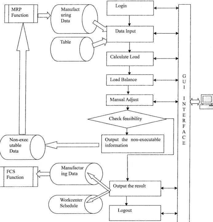
This CRP module uses the output of the MRP system as the input data. It will deploy the manufacturing order into the manufacturing process, then to calculate the operation time of the process. This module can dispose two kinds of the plan unit for the load calculation: work centre or work machine. The measure unit of the plan can be day or week. When we calculate the load of the plan unit, we also use the planned orders outputted by the posterior plan function (Finite Capacity Scheduling -FCS) together with the manufacturing orders, so that this load calculation is more accurate. After adding the load to the plan unit, we can do the auto-balance operation or the manual adjust operation to verify the feasibility of the plan of the tentative orders. If the plan is feasible, the module will output the manufacturing orders and produce the job orders. If the plan Is not feasible, it will output the useful information to the anterior fonction to review the tentative orders.

(24)

Figure 2.1 The workflow of the CRP module. MRP Function Non-exec utable Data Workcenter Schedule Login Data Input Calculate Load Load Balance Manual Adjust Manufactur / ing Data ( v».

V

Output the non-executable information

Output the result

Logout G U I N T E R F A C E

(25)

24

As showing in the figure 2.1, the CRP module is composed of 9 parts: 1. Login fonction

2. Data input fonction 3. Load calculation fonction 4. Load auto-balance fonction 5. Manual adjust fonction 6. Check the feasibility function

7. Output the non-executable information fonction 8. Data output fonction

9. Logout fonction

2.1 LOGIN FUNCTION

User must input user's ID and password for login the CRP fonction.

2.1.1 Input

Table 2.1 The following table shows the login input items. Input Item User's ID Password Login mode Cipher File Plant table Explain

The ID of the login user The password of the login user The mode of user's login. The list of user and password

According to the range of charge table, set the exclusive status in this table.

(26)

Workcenter table

Charge table Data source type

According to the range of charge table, set the exclusive status in this table.

Get the responsible range of work center from this table. Specify the type of the data source

2.1.2 Output

Table 2.2 The following table shows the login output message.

Output Item

Login success or not Type of the error

Explain

Return the result of the login. The number of the login error.

2.1,3 Detail Process

The process logic of the login function is described as :

The fields of user ID and password must be inputted.

Reading in the Cipher file, verify the user ID and password being correct or not. If the user ID or password is not correct, the error occurs, return the type of error. If the user ID and password are correct, then reading in the facility table and work center table and charge table from the specified data source.

From the charge table, get all responsible work centers of the user.

Verify the responsible work centers being used by other user. If it is the case, return an error.

If there is no the responsible work center being used by other user, set the status of the work center to exclusive.

(27)

26

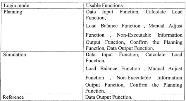
According to the user's login mode, we can restrict the CRP fonctions which user can be used. The following table shows this limit.

Table 2.3 Login mode Login mode

Planning

Simulation

Reference

Usable Functions

Data Input Function, Calculate Load Function,

Load Balance Function , Manual Adjust Function , Non-Executable Information Output Function, Confirm the Planning Function, Data Output Function.

Data Input Function, Calculate Load Function,

Load Balance Function , Manual Adjust Function , Non-Executable Information Output Function, Confirm the Planning Function.

Data Output Function.

2.2 DATA INPUT FUNCTION

This module reads the manufacturing orders produced by MRP from the data source into memory. At the same time, it completes the same operation with the part table, work center table, Calendar table etc.

2.2.1 Input

Table 2.4 Input items of the data input fonction Input Item

Manufacturing Order Table Manufacturing Divided Order

Note

Read into memory Read into memory

(28)

Table

Working Order Tale Part Table

Device Table Process Table

Process Sequence Table Valid Process Sequence Table Calendar Table

Working Shift Table Working Shift Type Table Non-work Period Table Producible Work center Table

Read into memory Read into memory Read into memory Read into memory Read into memory Read into memory Read into memory Read into memory Read into memory Read into memory Read into memory

2.2.2 Output

The following table shows the data input result. Table 2.5 Output items of the data input function Output Item

Data input success or not Type of the error

Explain

Return the result of the Data input. The number of the Data Input error.

2.2.3 Detail Process

Because the work center table and the responsible work center table are already read into memory when user logged into this module, all the rest tables are got into memory from the specified data source. Verifying the correctness of the tables must be processed at the time of reading of the tables. Database is as the default data source, if the user wants to read data from the other data source, it must be specified in the parameter file.

(29)

28

2.3 CALCULATE LOAD FUNCTION

The load calculation of the measure unit is taken by using the data read from the data source. There are two kinds of the work area for the load calculation: the work center and the work machine. We use the manufacturing time of each process deployed by the manufacturing order to calculate the workload. This function also uses the information of the process of the planned order in the posterior function (FCS) in order to achieve the high accurate calculation of the load.

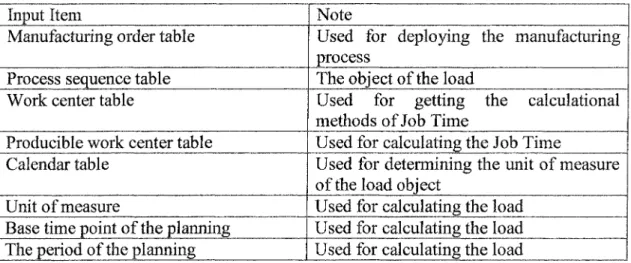
2.3.1 Input

Table 2.6 Input items of the calculate load function Input Item

Manufacturing order table Process sequence table Work center table

Producible work center table Calendar table

Unit of measure

Base time point of the planning The period of the planning

Note

Used for deploying the manufacturing process

The object of the load

Used for getting the calculational methods of Job Time

Used for calculating the Job Time

Used for determining the unit of measure of the load object

Used for calculating the load Used for calculating the load Used for calculating the load

2.3.2 Output

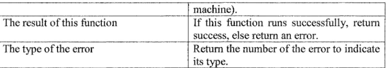
Table 2.7 Output items of the calculate load function Output Item

Information of the calculated load and the report of the load

Note

The load information of every unit of the measure (each work center or each

(30)

| machine). The result of this function

The type of the error

If this fonction runs successfully, return success, else return an error.

Return the number of the error to indicate its type.

2.3.3 Detail process

First of all, we check the input manufacturing orders whether they are the object to calculate the load or not. If they are the object to calculate, then deploy the process of this manufacturing order and calculate the job time of each process according to the unit of measure. We assume that infinite capacity exists at each of these work centers to satisfy this calculated. We use the processes that are determined by FCS fonction for the high precision load calculation.

2.3.3.1 Verification of the manufacturing order

The LFT (Latest Finish Time) of the manufacturing order must be later than the base time point of the planning. The EST (Earliest Start Time) of the manufacturing order must be in the period time of the planning. The table of 2.8 shows the detail.

Table 2.8 The object to calculate load The range of the manufacturing order

The LFT (Latest Finish Time) of the manufacturing order < the base time point of the planning

The object to calculate load No

(31)

30

The base time point of the planning <= the EST (Earliest Start Time) of the manufacturing order < (the base time point of the planning^- the period of the planning)

(The base time point of the planning+ the period of the planning) <= the EST (Earliest Start Time) of the manufacturing order

Yes

No

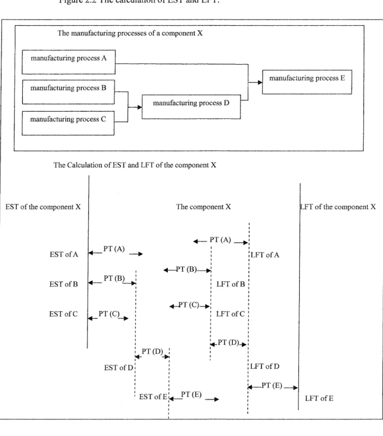
2.3.3.2 Deploying the manufacturing process

By using the process sequence table? the manufacturing process is deployed from the

manufacturing order of the component. The EST and LFT of each process are generated according to the production time of the process. The following tables figure out the method of this calculation.

Table 2.9 The calculation of LFT (Backward scheduling logic) The manufacturing process

The last manufacturing process The rest manufacturing process

The calculation of LFT The LFT of the last process

The LFT of the rest process is earliest time among all the subtraction of LFT with its production time (LFT -production time) .

Table 2.10 The calculation of EST (Backward scheduling logic) The manufacturing process

The earliest manufacturing process The rest manufacturing process

The calculation of EST

The earliest start time of the first manufacturing process.

The EST of the rest manufacturing process is latest time among all the subtraction of EST with its production time (EST - production time).

The concrete demonstration of the calculation of EST and LFT is shown in figure 2.3. In this figure PT means Production Time.

(32)

Figure 2.2 The calculation of EST and LFT.

The manufacturing processes of a component X

manufacturing process A

manufacturing process B

manufacturing process C

The Calculi

EST of the component X

EST of A

EST of B

EST of C

manufacturing process D 1

ition of EST and LFT of the component X

The component X ^ PT(A) ; <*— — • ; ; LFT of B ; ^_PT (C)->! PT(C) i ! LFT of C i i !PT(D) : : ESTofD; ! manufacturing process E LFT of A LFT of D LFT of the component X LFT of E

(33)

32

2.3.3.3 The calculation of production time of the manufacturing process

The production time of the manufacturing process equals the sum of the product of rated production time of the process and the mount of components and the prepare time. The formulation is:

The production time = (rated production time of the process)*( the mount of components) + the prepare time.

2.3.3.4 The different capacities and loads

The object to be calculated the load can be work center or work machine of the manufacturing area, at the same time, the measure unit of the load can be hour or day, this can be set in the parameter file. In the case of work center, the calculation of load is completed according to the measure unit defined in the process sequence table. In the case of work machine, the rules of selection the work machine to load must be followed are:

Select the machine in the top-priority work center.

In the same work center, select the top-priority machine. If it is overload, then select the next top-priority machine.

(34)

2.3.3.5 The calculation of the standard capacity

Using the following method to calculate the standard capacity of the different machines:

The standard capacity of the current measure unit = The sum of production time of every day according to the measure unit.

The production time of the current day = QXthe shift production time of the current day of the machine) + append production time )* capacity coefficient

The standard capacity of the different work centers is shown as the formula:

The standard capacity of the current measure unit = X(the standard capacities of all machines that are belong to the current center).

2.3.3.6 The discrimination of manufacturing area

If the object to be calculated the load is work center, the load of different machines can not be identified. Whereas in the case of the calculation load of the machine, the load of every work center can be discriminated, because the load of the center equals to the sum of the loads of all machines that are belong to the current center.

(35)

34

2.3.3.7 Getting the information from the fonction of the posterior planning (FCS)

This calculation load fonction also gets the information from the fonction of the posterior planning (FCS). It uses the confirmed production orders of the posterior planning to calculate the load so that this calculation is more accurate. The table 2.11 shows the detail.

Table 2.11 The information introduced from the posterior planning (FCS) Information

The ID of process sequence of the current process

The ID of manufacturing order which includes the current process The start time of the process

The end time of the process

The ID of the machine of the current process

The ID of planned order introduced from the fonction of the posterior planning must be same as the ID of current manufacturing order. The ID of process sequence of the planned order must be the same as the ID of process sequence of the current manufacturing process deployed from the current manufacturing order. The following table shows the information:

Table 2.12 The information deployed from the planned order Information of the

process

Earliest start time Latest finish time

Setting information

The start time of the process of the planned order The finish time of the process of the planned order

(36)

Production time The finish time of the process of the planned order- the start time of the process of the planned order

The object to calculate the load

The machine which its ID is uniform to the ID of the machine of the current manufacturing order.

Or the work center that the machine of the planned order belongs to. The ID of the machine is uniform to the ID of the machine of the current manufacturing order

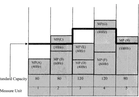
2.3.3.8 The example of the loads

The figure 2.3 shows an example of the loads. Here MP means Manufacturing Process.

Figure 2.3 An example of the load.

Standard Capacity Measure Unit MP{A) (40Hr) 80 MHO (40Hr) MPfB) (60Hr) 80 2" MP(E) (40Hr) MP(D> (40Hr) 120 MI^G) (80Hr) • MP(F} (60Hr) 120 MP (H) (IQOHr) 80 5

(37)

36

2.4 AUTO-BALANCE FUNCTION

For the calculated load, the auto-balance fonction of the load is processed at the base of the standard capacity. The result of the adjustment of the manufacturing process of this auto-balance fonction can not be as the output of the CRP module.

2.4.1 Input

Table 2.13 The input items of the Auto-balance fonction. Input Item

The information of Calculate Load Function

Work Center Table

Note

Load information of the work center

To get the calculate measure of the job time

2.4.2 Output

Table 2.14 The output items of the Auto-balance function. Output Item

Information of the calculated load and the report of the load

The result of this fonction The type of the error

Note

The load information after auto-balance fonction

If this fonction runs successfully, return success, else return an error.

2.4.3 Detail process

(38)

manufacturing orders using backward scheduling. Backward scheduling logic will calculate each operation backwards from the manufacturing order or planned order.

The algorithm of the auto-balance load fonction we used is simple. In the case of calculation of work center, the auto-balance load fonction is processed with the work center as measure unit. Whereas in the case of calculation of work machine, the auto-balance load fonction is processed with the work machine as measure unit. The loads can only be transferred between the machines in the same work center. For the complicate auto-load fonction, such as the transference of loads between machines in different work centers, we don't take into account.

The detail algorithm of auto-balance load fonction is illustrated by two examples shown in Figure 2.4-2.7.

These two examples are based on the assumption that the sequence of EST of every manufacturing process is the same as the sequence of the English letters used to express the process. So the EST of the manufacturing process A is the earliest, and that the EST of the process H is the latest. Moreover, The EST of each manufacturing process is earlier than the base point of the planning.

(39)

38

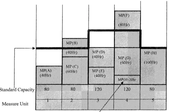
Figure 2.4 The load of the each measure unit.

Standard Capacity Measure Unit MP(A) <40Hr) 80 - 1 MP(B) (40Hr) (60Hr) 80 "1 "*" MP(D> (40Hr) MP<E) (40Hr) 120 3 MP(F) MF(O) (60Hr) 120 MP(H) (lOOHr) 80 •"' 5 " " •

As showing in the figure, because the capacity of the measure unit is over load compared with the standard capacity, it must be taken the auto-balance process of the load. Taking the latest measure unit 5 as the first object to be treated with, the over load 20(Hours) of the manufacturing process of the measure unit 4, as showing in the following figure.

(40)

Figure 2.5 The overload 20(Hr) is transferred to measure unit 4. Standard Capacity Measure Unit MPIA) <40Hr) 80 -' I-MF(B) (40Hr) MP(C) (60Hf) 8Û . — ^ ^ — ^ ^ MF(D) (40Hr) MP{E) (40Hr) 120

V

MP(F) (8QHr) MP(G) (60Hr) MP(U)2Qhf / 120 MP{H) (lOOHr) 80 overload 20(Hr) is transferred to 4

After this transference to the measure unit 4, the loads of the measure unit 5 is under the standard capacity, but the load of the measure unit 4 is over the standard capacity. So the transference of load begins from the earliest EFT of the manufacturing process F, the over load of 40 Hours moves ahead. This is shown in the following figure.

(41)

40

Figure 2.6 The overload 40(Hr) is transferred to the measure unit 3.

Standard Capacity Measure Unit MP(A) (40Hr) 80 MP(B) (40Hr) MP<C) (60Hr) 80

V

MP(D) (40Hr) MP(E) (40Hr) MP(F) l40Hr) /l20 • 3 MP(F> (80Hr) MP(6) (60Hr) MP(H)20hr 120 4' MP(H) (lOOHr) 80 5 '

overload 40(Hr) is transferred to the measure unit 3

Because the load of the measure unit 3 is not over the standard capacity? the measure

unit 2 is treated directly. The over load of the measure unit 2 is 20 hours. So the transference of load begins from the earliest EFT of the manufacturing process B. Figure shows this case.

(42)

Figure 2.7 The overload 20(Hr) is transferred to the measure unit 1. Standard Capacity Measure Unit / MP(A) (40Hr) MftB)20hr

A

/ t MP(8)(40 MPrcj <60Hr) 80 MP(D) (40Hr) (40Hr)

unv)

(40Hr) 120 .->

•II

Illiiiiiftilp i ll^^llllllijilii i MP(G) (60Hr) MPCH)20hr 120 MP(Hî <IOÔHr> 5

overload 20(Hr) is transferred to the measure unit 1

There is not measure unit ahead of the measure unit 1, so the auto-balance process finish.

Because the load of the measure unit 1 is under the standard capacity5 so the planning

of this work center is executable.

(43)

42

Figure 2.8 The load of the each measure unit.

Standard Capacity Measure Unit MP(A) (40Hr) 80 M.P(0) (4QHv) MP(C) (40Hr) MP(D) (60Hr) 80 T MP(E) (40Hr) MP<F) <40Hr) 120 MP(G) (S'OHr) MP(H) (60Hr) 120 MP (1) (lOOHr) 80

The procedure of auto-balance of the load in this example is similar with that is in the example 1 until the measure unit 2.

Figure 2.9 The load transference until the measure unit 2.

Standard Capacity Measure Unit MP(A) (40Hr) 80 1 ~"" MP(B) (40Hr) MP(C) ' MP(D) (60Hr) 80 MP (E) (40Hr) MP(F) (40Hr) MP(G) (40Hr) 120 MP(G) (80Hr) MP(H) (60Hr) MP(l)2t)hr 120 MP(1) (lOOHr) 80 5

(44)

Because the load of the measure unit 2 is over the standard capacity, the transference of load begins from the earliest EFT of the manufacturing process B. In this case, the load of the manufacturing process B is less than the over part of the load of measure unit 2. So the total load of the manufacturing process B is transferred to the measure unit 1. The figure 2.10 shows this case.

Figure 2.10 Transfer the entire load of manufacturing process B to the measure unit 1. Standard Capacity Measure Unit MP(A) <40Hr) MP(B) <40Hr) {60Hrt 80 MP(E) (40Hr) MP(F) (40Hr) MP(G) <40Hr) 120 MP(G) iSOHr) MPtH) (6tiHr) 120 MP(f) (JOOHr) 80

Transfer the entire load of manufacturing process B to the measure unit 1

The load of the measure unit 2 is still over load even though the entire load of manufacturing process B is transferred to the measure unit 1. So the over load 20 Hours of

(45)

the manufacturing process C must be moved to the measure unit 1.

Figure 2.11 Transfer the overload to the measure unit 1.

Standard Capacity Measure Unit MR A) (40Hr) MF(C) 2Ohr MP(C) (4UHr) MP (D) <60Hr) 80 (40Hr) MP<F) (40Hr) MP(G) (40Hr) 120 MP(G) (SOHr) MP<H) (6GHr> MP(t>20hr 120

Transfer the overload to the measure unit 1

MP<!)

(ICMIHr)

80

—r

44

There is no measure unit ahead of the measure unit 1? so the auto-balance of the load

finishes. Because the load of the measure unit 1 is over the standard capacity, in this case the planning of the work center is non-executable.

(46)

2.5 MANUAL ADJUST FUNCTION

It is required to offer the means of manual adjust fonction after the load calculation. The conceivable operations of the manual adjust fonction are listed in the following table.

Table 2.15 The operations of the manual adjust fonction. Operation Transfer Divide Combine Append Delete

Modify the quantity of the product

Modify the schedule and the shift type

Undo

Note

Transfer the load from one manufacturing process to an other.

Divide one manufacturing order into two orders. Combine two divided orders to one manufacturing order

Append manufacturing orders. When the manufacturing orders are appended, the validity of MRP is not guaranteed.

Remove the manufacturing orders. When the manufacturing orders are deleted, the validity of MRP is not guaranteed.

Modify the quantity of the product of the manufacturing order. When this amount is modified, the validity of MRP is not guaranteed. Modify the day-off or the overtime of the facility to adjust the standard capacity of the work center, so that the load is under the standard capacity. Recover the current manual operation.

2.5.1 The transference of the load

The specified load of the manufacturing process is transferred to the appointed plan unit or work center. There are two kinds of the transference.

(47)

46

2.5.1.1 The transference of the load between the work centers

The possible moveable work centers are only those which are corresponding to the current work sequences defined in the producible work center table. This transference can not be performed to the work centers of the other facility. If the moveable status of the facility is set to false, an error will occur.

2.5.1.2 The transference of the load between the work machines

The load calculation is performed using the work machine unit. The possible moveable work machines are only those which are corresponding to the current manufacturing process defined in the producible work center table. This transference can not be performed to the work machines of the work center of the other facility. If the moveable status of the machine is set to false, an error will occur.

2.5.1.3 Input

Table 2.16 The input items of the transference of the load. Input Item

ID of the manufacturing order

ID of the divided manufacturing order

ID of the manufacturing process ID of work center or machine Date

Note

The ID of the manufacturing order which includes the manufacturing process, its load is transferred.

The ID of the divided manufacturing order which includes the manufacturing process, its load is transferred.

The ID of the manufacturing process, its load is transferred.

The ID of the work center or machine to be transferred.

The date of manufacturing process to be transferred.

(48)

2.5.1.4 Output

Table 2.17 The output items of the transference of the load. Output Item

ID of manufacturing process The load information

The result of this operation The type of the error

Note

The ID of the manufacturing process after the transference.

The load infonnation of the work center or machine after the transference.

If this function runs successfully, return success, else return an error.

2.5.2 The division of the manufacturing order

The manufacturing order is divided by the specified quantity of the order. At the same time as the manufacturing order is divided, all the manufacturing processes deployed from the current manufacturing order are divided the same quantity. The specified quantity the order must be ranging between 0 < divided quantity < the quantity of the order before division.

After the division, the information of the new manufacturing order is shown in the table.

(49)

48

Table 2.18 The information of the new manufacturing order of the division of the manufacturing order. Items ID of the manufacturing order ID of the divided manufacturing order ID of the component ID of the work center EST

LFT Quantity

The manufacturing order 1 after division

Same as the manufacturing order before division

The specified quantity

The manufacturing order 2 after division

The minimum value not used of the divided manufacturing order for the same manufacturing order ID.

The quantity before division - quantity.

2.5.2.1 Input

Table 2.19 The input items of the division of the manufacturing order.

Input Item

ID of he manufacturing order

ID of the divided manufacturing order Quantity

Note

The ID of the manufacturing order to be divided.

The ID of the divided manufacturing order to be divided.

The quantity of the manufacturing order after division.

(50)

2.5.2.2 Output

Table 2.20 The output items of the division of the manufacturing order. Output Item

Manufacturing order 1 Manufacturing order 2 The load information The result of this operation The type of the error

Note

The manufacturing order 1 after division The manufacturing order 2 after division. The load information of the work center or machine after the division.

2.5.3 The Combination of the manufacturing order

The combination of the manufacturing order is performed by two specified manufacturing orders. After combination these two manufacturing orders, all the manufacturing processes deployed from these two manufacturing orders must be combined together. The quantity of the manufacturing order after combination is the sum of two combined manufacturing orders. The ID of the divided manufacturing order is the minor value of these two IDs of the divided manufacturing orders. The other information except the quantity and the ID of the divided manufacturing order will inherit the same information of the manufacturing order. The combination can only be performed between the divided manufacturing orders which have the same manufacturing order ID.

(51)

50

2.5.3.1 Input

Table 2.21 The input items of the combination of the manufacturing order. Input Item

ID of the manufacturing order 1 ID of the divided manufacturing order

1

ID of the manufacturing order 2 ID of the divided manufacturing order 2

Note

The ID of the manufacturing order 1 to be combined.

The ID of the divided manufacturing order 1 to be combined.

The ID of the manufacturing order 2 to be combined.

The ID of the divided manufacturing order 2 to be combined.

2.5.3.2 Output

Table 2.22 The output items of the combination of the manufacturing order. Output Item

Manufacturing order The load information The result of this operation The type of the error

Note

The manufacturing order after the combination.

The load information of the work center or machine after the division.

2.5.4 The accession of the manufacturing order

The accession of the new manufacturing order is based on the specified information of the manufacturing order. After the new manufacturing order is created, all the processes of the manufacturing order are generated. At the same time, the load calculation of the manufacturing process is also performed.

(52)

2.5.4.1 Input

Table 2.23 The input items of the accession of the manufacturing order. Input Item

All the necessary information of new manufacturing order

Note

Input the necessary information for creating the new manufacturing order.

2.5.4.2 Output

Table 2.24 The output items of the accession of the manufacturing order. Output Item

Note

The new manufacturing order after the accession.

The load information of the work center or machine after the accession.

2.5.5 The deletion of the manufacturing order

Deleting a manufacturing order is performed by specified its ID, at the same time, all manufacturing processes deployed by the current manufacturing order are also removed.

2.5.5.1 Input

Table 2.25 The input items of the deletion of the manufacturing order. Input Item

ID of the divided manufacturing order

Note

The ID of the manufacturing order to be removed.

The ID of the divided manufacturing order to be deleted.

(53)

52

2.5.5.2 Output

Table 2.26 The output items of the deletion of the manufacturing order. Output Item

Note

The manufacturing order to be deleted. The load information of the work center or machine after the deletion.

2.5.6 The modification of the quantity of the manufacturing order

Modifying the quantity of a manufacturing order is performed by specified its new quantity at the same time, all manufacturing processes deployed by the current manufacturing order are also modified.

2.5.6.1 Input

Table 2.27 The input items of the modification of the quantity of the manufacturing order.

Input Item

ID of the divided manufacturing order The Quantity

Note

The ID of the manufacturing order to be modified.

The ID of the divided manufacturing order to be modified.

The new quantity of the manufacturing order.

(54)

2.5.6.2 Output

Table 2.28 The output items of the modification of the quantity of the manufacturing order.

Output Item

Note

The manufacturing order to be modified its quantity.

The load information of the work center or machine after the modification.

2.5.7 The modification of the schedule and the shift type

The objective of modifying the day-off or the overtime of the facility is to adjust the standard capacity of the work center, so that the load is under the standard capacity. There are four types of the modifications listed in the following table.

Table 2.29 The operations of the modification of the shift. Operation

Modify the shift type

Append the overtime

Append the day-off Delete the day-off

Note

Modify the shift type of the specified work center or machine to the other type of the shift.

Append the overtime of the work center will change the overtime of all machines of this work center.

Append the day-off of the work machine. Delete the day-off of the work machine.

(55)

54

5.2.8 Undo operation

For the manual operations, the Undo mechanism is necessary. In one case, if the input parameters of the manual operation are not correct, the Undo operation must be performed. In the other case, when several manual operations are executed, we want to recover the one of them. So the Undo mechanism can satisfy this requirement.

The level of the Undo operation can be set in the parameter file.

2.6 CHECK THE FEASIBILITY OF THE PLANNING

This module is to check the load of the measure unit whether is under the standard capacity or not.

2.6.1 Input

Table 2.30 The input items of the verification of the feasibility of the planning. Input Item

ID of the work center (machine) The load information

Note

Check the feasibility of planning of the specified work center (machine).

Use the load information to check the feasibility.

2.6.2 Output

Table 2.31 The output items of the verification of the feasibility of the planning. Output Item

The result of this operation Arrange the measure unit

Note

If the planning of the work center is executable, return true, else return false. General view of the non-executable measure unit.

(56)

2.7 OUTPUT THE NON-EXECUTABLE INFORMATION

If the load of the work center is overload, output the non-executable load information.

2.7.1 Input

Table 2.32 The input items of the output of the non-executable information. Input Item

ID of the work center (machine) The load information

Note

Check the feasibility of planning of the specified work center (machine).

Use the load information to output.

2.7.2 Output

Table 2.33 The output items of the output of the non-executable information. Output Item

The non-executable load information

The result of this operation The type of the error

Note

If the planning of the work center is non-executable, save the manufacturing order to local file.

2.8 DATA OUTPUT

This CRP module finally generates the job order to reflect the result of the load adjustment and the update of the manufacturing order.

2.8.1 Input None.

(57)

2.8.2 Output

Table 2.34 The output items of the data output function.

2.9 LOGOUT

56

Output Item

The manufacturing order The job order

The shift

Note

Reflect the adjustment of load Reflect the adjustment of load Reflect the adjustment of load

Logout function exits the current CRP module and saves the necessary information. There is no input data and output data involved in this part.

(58)

This chapter will discuss the data input? the load calculation and manual adjust parts.

Each part contains an associated class for which their behavior and data will describe. The class descriptions will include a statement of purpose and description of both the public and private declarations. The other parts (login5 data output and Undo fonction) will not be

discussed.

3.1 THE UML OF THE CRP MODULE

This CRP module contains 9 domains as showing in figure 3.1. Each domain comprises several classes. The Figure 3.1 illustrates the UML of these classes.

(59)

(60)

3.2 THE DATA INPUT CLASS

The data input class will be addressed first because it gets all necessary data into memory from the database for the later use. The corresponding 'ZRDatalnput5 class allows

us to dynamically build all tables in memory. The default data source is database. It also allows the user to read the data from other data source specified in the configuration file. This class contains all of the information needed to calculate the load of the work area.

Table 3.1 describes the private variable declarations in the ZRDatalnput class. Private variables are accessible only to member fonctions of the class.

Table 3.1 The private variable declarations in the ZRDatalnput class. Declaration Connection conn String logFileName BufferedWriter bufWriter Vector vComponent Vector vWorkingProcedure Vector vSequence Vector vValidSequence Vector vMachine Vector vWorkCenter Vector vShiftType Vector vShift Vector vDayOff Description

The connection with the data source The file name of the log file

Used to write file.

Data storage vector that holds the records data of the component table.

Data storage vector that holds the records data of the Manufacturing process table. Data storage vector that holds the records data of the Working Sequence table. Data storage vector that holds the records data of the Working Sequence table. Data storage vector that holds the records data of the Work Machine table.

Data storage vector that holds the records data of the Work Center table.

Data storage vector that holds the records data of the Shift Type table.

Data storage vector that holds the records data of the Shift table.

Data storage vector that holds the records data of the Day Off table.

(61)

60 Vector vMnfOrder Vector vMnfDividedOrder Vector vCalendar Vector vPlannedOrder Vector vFacility Vector vCharge Vector vUserlnfo

Data storage vector that holds the records data of the Manufacturing order table. Data storage vector that holds the records data of the Manufacturing divided order table.

Data storage vector that holds the records data of the Calendar table.

Data storage vector that holds the records data of the Planned Order table.

Data storage vector that holds the records data of the Facility table.

Data storage vector that holds the records data of the Charge table.

Data storage vector that holds the records data of the User table.

Each vector contains the records data of the corresponding table. It uses the base class of the record. For example, the Vector vMnfOrder uses the MnfOrderRecord class which is coiresponding with one record of the Manufacturing order table.

The following table shows the ZRDatalnput public fonction declarations. These fonctions are the users interface to the load calculation fonction.

Table 3.2 The public fonction declarations in the ZRDatalnput class. Declaration

int getAUTable

Vector getVectorComponent Void setVectorComponent The other getVectorXXX?

setVectorXXX fonctions

corresponding to the vectors listed in Table 3.1

Description

Read all record data from the data source into corresponding vector. If the reading operation runs successfully, this fonction return 0, else return a number to indicate the type of the error.

Get the private variable vComponent of the ZRDatalnput.

Set the vector to the private variable vComponent of the ZRDatalnput. Get the vXXX vector from ZRDatalnput or set the vector to vXXX.

(62)

Table 3.3 shows the private function declarations of the ZRDatalnput class. Declaration

int getComponentTable

int checkComponentRecord

The other getXXXTable and checkXXXRecord fonctions corresponding to the vectors listed in Table 3.1

Description

Read the record data from the Component table into the corresponding vector vComponent. If the reading operation runs successfolly5 this fonction return 0,

else return a number to indicate the type of the error.

When this fonction reads the Component data from the data source, it must be taken the verification of correctness of the Component record.

Read the record data from the XXX table into the corresponding vector vXXX. If the reading operation runs successfully, this fonction return 0? else return a

number to indicate the type of the error.

3.3 LOAD CALCULATION CLASS

The ZRLoadCalcul class is the most important class in this module, because it performs not only the load calculation of the work area according to the measure unit, it also takes the task of auto-balance of the load. The load calculation is performed by using the work time of each manufacturing process deployed by the manufacturing order.

The auto-balance load fonction will process and reschedule all open and planned manufacturing orders using backward scheduling. Backward scheduling logic will calculate each operation backwards from the manufacturing order or planned order.

(63)

62

Table 3.4 shows the private variable declarations in the ZRLoadCalcul class. Declaration ZRDatalnput datalnput int intCapacityUnit Date datePlanBase int intPlanDucration Date dateBeginTime Hashtable htMachine Hashtable htWorkCenter Hashtable htMachineWeek Hashtable htWorkCenterWeek Hashtable htAHProcedure Description

The data input class The unit of the capacity The base point of the plan The period of the plan The start date of the plan

Data storage hashtable that holds all machines information.

Data storage hashtable that holds all Work Centers information.

Data storage hashtable that holds all machines information. The capacity unit is week.

Data storage hashtable that holds all work center information. The capacity unit is week.

Data storage hashtable that holds all manufacturing processes information.

The following table shows the ZRLoadCalcul public fiinction declarations. These functions are the users interface to the load calculation fiinction.

Table 3.5 The public function declarations in the ZRLoadCalcul class. Declaration

ZRLoadCalcul loadCalculation

autoBalance

Description

Constructor function, in this function the initialization task is done.

This is the core function in this CRP system, it will dévide manufacturing order into manufacturing process, and do load calculation operation.

It is this fiinction that does the auto-balance of the load. It compares the load of the current measure unit with its standard capacity to determine the under load or over load.

(64)

getLoadlnformation

getUnexecutablelnformation

This fonction returns all load information of the work center or work machine. This fonction returns all load information of the measure unit that their capacity are over load

Table 3.6 The private fonction declarations of the ZRLoadCalcul class. Declaration initWorkCenterByDay initWorkMachineByDay initWorkCenterByWeek initWorkMachineByWeek Description

Initialize the WorkCenter by day5create

instances of ZRWorkCenter class and put them into Hashtable variable htWorkCenter

Initialize the WorkMachine by day,create instances of ZRWorkMachine class and put them into Hashtable variable htWorkMachine

Initialize the WorkCenter by week5create

instances of ZRWorkCenter class and put them into Hashtable variable htWorkCenterWeek

Initialize the Machine by week5create

instances of ZRMachine class and put them into Hashtable variable htMachineWeek

3.4 MANUAL ADJUST CLASSES

As discussed in chapter 5, the manual adjust part consists of 8 operations. These operations are base on the interface 'ZRManualAdjust9. Here I will discuss one class for

illustration: the class ZRLoadTransfer. The other classes are similar to this class. You can find them in the Index C.

(65)

64

3.4.1 The interface ZRManualAdjust

The following table shows the public fonctions placed in the interface ZRManualAdjust.

Table 3.7 The public functions placed in the interface ZRManualAdjust. Declaration Void setParameter Vector getParameter Hashtable[] getExistedRecords int changeExistedRecords Description

This interface sets the necessary parameters of the manual operation. This interface gets the input parameters of the manual operation.

This interface gets all necessary existed hashtable to perform the manual operation.

This interface performs the manual operation.

3.4.2 Load transfer class

ZRLoadTransfer class is corresponding to the load transference operation. There are two kinds of the transference: the load between the work centers and the load between the work machines.

Table 3.8 Shows the private variable declarations in the ZRLoadTransfer class. Declaration ZRDatalnput zrDatalnput ZRLoadCalcul zrLoadCalcul Boolean moveFlag Vector vLoadTransferlnfo Hashtable[] existedOrderRecords Description

The class instance of class ZRDatalnput The class instance of class ZRLoadCalcul The flag of the transference operation The vector stores the parameter list. The existed manufacturing order hashtable.

(66)

Table 3.9 shows the public variable declarations in the ZRLoadTransfer class. Declaration

OperationObject oo UndoList ul

Description

The class object is prepared for the Undo operation.

The Undo list used for the Undo operation.

Because the class ZRLoadTransfer extends the interface ZRManualAdjust, the public functions of this class are the same as shown in the table 6.4.1.

3.5 CRP TASK CLASS

I design the ZRCRPTask class to provide the interfaces of all of the tasks described in the previous chapters. This is for two purposes. The first is that the CRP module will work as a whole to integrate to the ZRERP system. The second is that this module can work independently, so we can use this class to interact with the GUI classes.

Table 3.10 shows the private variable declarations in the ZRCRPTask class.

Declaration ZRConnection crpconn ZRDatalnput zrDatalnput ZRDataOutput zrDataOutput ZRLogin zrLogin ZRLoadCalcul zrLoadCalcul ZRLoadTransfer zrLoadTransfer ZROrderDivide zrOrderDivide ZROrderAppend zrOrderAppend Description

Open the connection with the data source The class instance of class ZRDatalnput The class instance of class ZRDataOutput The class instance of class ZRLogin The class instance of class ZRLoadCalcul The class instance of the class ZRLoadTransfer to perform the load transference operation of manual adjust. The class instance of the class ZROrderDivide to perform the load division operation of manual adjust. The class instance of the class ZROrderAppend to perform the order append operation of manual adjust.