The relationship between productivity and tree-ring growth in boreal coniferous forests

issn 1239-6095 (print) issn 1797-2469 (online) helsinki 28 november 2014

Editor in charge of this article: Eero Nikinmaa

the relationship between productivity and tree-ring growth in

boreal coniferous forests

Guillermo Gea-izquierdo

_{*, Yves Bergeron}

_{, Jian-Guo huang}

_,

marie-Pierre lapointe-Garant

_{, John Grace}

_{and Frank Berninger}

1) _{Centre d’Étude de la Forêt (CEF), Département des Sciences Biologiques, Université du Québec à} Montreal, CP 8888 Succ. Centre Ville, Montreal (Qc), H3P 3P8, Canada (*corresponding author’s e-mails: gea-izquierdo@cerege.fr; guigeiz@gmail.com)

2) _{CEREGE UMR 7330, CNRS/Aix-Marseille Université, Europole de l’Arbois, BP 80, F-13545} Aix-en-Provence Cedex 4, France

3) _{Université du Québec en Abitibi-Témiscamingue, 445 Boulevard de l’Université, Rouyn-Noranda,} Québec, J9X 5E4, Canada

4) _{School of GeoSciences, The University of Edinburgh, The King’s Buildings, West Mains Road,} Edinburgh EH9 3JN, UK

5) _{Department of Forest Sciences, P.O. Box 27, FI-00014 University of Helsinki, Finland} 6) _{South China Botanical Garden, Chinese Academy of Sciences, Guangzhou, 510650, China} Received 20 May 2013, final version received 14 Mar. 2014, accepted 15 Mar. 2014

Gea-izquierdo, G., Bergeron, Y., huang, J. G., lapointe-Garant, m. P., Grace, J. & Berninger, F. 2014: the relationship between productivity and tree-ring growth in boreal coniferous forests. Boreal Env.

Res. 19: 363–378.

Ecosystem productivity estimated with a model calibrated with eddy-covariance data was related to tree-ring growth of two different boreal conifers along a latitudinal gradient. The relationship between ecosystem productivity and growth changed with species and site. Greater photosynthesis in spring and summer increased annual anomalies of radial growth in both species, and the response of growth to productivity was earlier in warmer southern stands particularly for pine. Radial growth of jack pine increased in the long-term with higher productivity, whereas this relationship was more reduced in black spruce. This could express species-specific differences in carbon allocation strategies but likely it is a consequence of the limiting marginal soils where spruce is found in the south. Only tree-rings of jack pine at some sites showed certain potential as direct proxies for ecosystem productivity at the low and high-frequency responses.

Introduction

Climate warming and the increase in atmos-pheric-CO₂ concentrations cause changes in forest growth and ecosystem productivity. There are reports of contrasting growth responses to warming over recent decades in different types of forests. Although some boreal species show

negative growth trends in response to recent climate change (Hoofgaard et al. 1999, D’Arrigo

et al. 2004), net ecosystem productivity in boreal

and temperate conditions is generally expected to increase with increasing temperatures (Myneni

et al. 1997, Boisvenue and Running 2006).

Forest growth measurements and models assume that there is a close connection between the stem

growth of a tree and its carbon balance (e.g. Running 1994, Le Roux et al. 2001, Zweifel et

al. 2010). Variations in the net ecosystem

pro-ductivity can be measured and modelled from networks of eddy-covariance towers (Kramer

et al. 2002, Baldocchi et al. 2003, Bergeron et al. 2007) which provide useful insights into

the carbon balances of ecosystems and their ecological drivers. However, since these towers are expensive to operate they provide limited temporal and spatial coverage of ecosystem carbon balances. Productivity estimates can also be derived from biometric-ecological inventory methods but these methods present similar short-comings as those for eddy-covariance stations (Ehman et al. 2002, Gough et al. 2008, Ohtsuka

et al. 2009).

Tree-ring records obtained using dendrochro-nological methods (Cook and Kairiukstis 1990) could be a key tool to extend carbon balances or ecosystem productivity to larger time scales and areas. Tree rings would be a useful comple-ment to direct ecosystem productivity estimates since they extend both spatially and temporally beyond the directly measured data of net eco-system exchange from flux towers. Addition-ally, a large quality checked archive of tree ring data is readily available from databases such as the International Tree-Ring Data Bank (ITRDB, http://www.ncdc.noaa.gov/paleo/treering.html). They have annual resolution and span many dec-ades of forest growth. Traditionally, empirical models where climatic variables are regressed against tree growth indices were employed to fit the relationship between climate and growth in dendrochronology. Several authors developed mechanistic approaches of annual tree ring for-mation with more comprehensive process-based models that are also able to take into account the non-linear response of growth to climate (Foster & Leblanc 1993, Berninger et al. 2004, Misson 2004, Vaganov et al. 2006, Drew et al. 2010). These models try to mimic not only the influence of climatic factors, but can also account for phe-nology, radiation, changes in transpiration and other ecophysiological processes involving car-bohydrate synthesis and allocation. The models perform well in explaining annual radial growth but generally not better than the classic,

empiri-cal approaches (Anchukaitis et al. 2006, Evans

et al. 2006, Shi et al. 2008).

Several authors compared tree-ring growth with estimates of net primary productivity from mechanistic models (Rathgeber et al. 2003, Ber-ninger et al. 2004, Girardin et al. 2008, Hari and Nöjd, 2009). Others studied the relationship between direct carbon flux estimates at eddy-covariance stations and tree-ring growth (Rocha

et al. 2006), flux estimates and cambial growth

(Zweifel et al. 2010) and flux estimates and bio-metric measurements of tree growth from per-manent plots (Ehman et al. 2002, Gough et al. 2008, Granier et al. 2008, Ohtsuka et al. 2009). If ecosystem carbon fixation and ecosystem pro-ductivity could be estimated from tree rings, then dendrochronological data might provide an effective tool for the spatial and temporal extrap-olation of micrometerological methods. How-ever, to our knowledge no study has analyzed the variability in the relationship between growth and ecosystem productivity along a climatic gra-dient, since existing studies are concerned with local relationships between growth of stands around eddy-covariance stations and direct eco-system flux measurements from the stations. Some agreement between ecosystem productiv-ity and radial growth has been reported, yet these studies suggest that unknown carbon allocation strategies may obscure the growth–carbon rela-tionship (Rocha et al. 2006, Gough et al. 2008, Ohtsuka et al. 2009). We analyzed the relation-ship between modeled ecosystem productivity and annual radial growth for two coniferous spe-cies sampled along a latitudinal (i.e. temperature and precipitation) gradient in eastern Canada. The growth data were originally published in Huang et al. (2010) who analyzed the relation-ship between the high-frequency of growth and climate using a classical empirical approach. Now we extend this work by using calculated ecosystem productivity as a covariate to inves-tigate whether tree rings can be used as indirect estimates of ecosystem productivity. We split growth into its low- (i.e. to analyze the long-term multidecadal trends) and high-frequency (i.e. to analyze the short-term, annual response) compo-nents to analyze this relationship in the short and the long terms.

Material and methods

Tree-ring data: disentangling high- from low-frequency of growth

We analyzed the relationship between annual radial growth and net and gross ecosystem exchange in two boreal species from eastern Canada: black spruce (Picea mariana) and jack pine (Pinus banksiana). They are dominant post-fire species widely distributed in North America. Jack pine generally occurs at xeric sites with sandy soil, and black spruce generally occurs at sites with poor soil covered by thick moss layers (see Table 1 for further description on the sampled sites). In the south, black spruce stands mostly co-occur with balsam fir (Abies

balsamea), red pine (Pinus resinosa) and white

pine (Pinus strobus). Jack-pine stands co-occur with black spruce and white birch (Betula

papy-rifera). In the north, monospecific pure stands of

both species are frequently found. Samples were collected from dominant trees in dense, mature, un-managed post-fire stands.

Increment cores were collected from 20 trees from nine locations on a latitudinal transect from 46°N to 54°N (Table 1 and Fig. 1). Cores were processed and analyzed to build annual series of

individual tree growth increments using standard dendrochronological methods (Cook and Kairi-ukstis 1990). Detrending methods in dendro-chronology can emphasize either the long- or short-term growth response. We therefore split the analysis of the relationship between eco-system productivity and growth in two: (1) a low-frequency analysis, using a variation of the regional curve standardization (RCS), which fits a single age-growth curve to all sites, and mixed models to study the response of growth to eco-system productivity in the long-term; (2) a high-frequency analysis of the growth response to ecosystem productivity on each site separately to study how growth at the nine individual sites responded to productivity in the short-term (i.e. to annual growth anomalies). In both analyses, we used mean site chronologies of growth indi-ces instead of individual tree growth series to pool out the influence of individual dendrometric features, thus making the growth indices compa-rable with estimates of ecosystem productivity. low-frequency analysis: I_Bai

For the low frequency analysis we used annual, basal area increments (BAI; see Fig. 2) with a

Table 1. characteristics of sampling sites and sampled stands (black spruce and jack pine) along the latitudinal

gradient from 46°n to 54°n in the eastern canadian boreal forest.

species lat. (°n), long. (°W) elevation stand types (m a.s.l.) slopes(°)/aspect sample type Black spruce 45°59´, 77°28´ 183 Uneven-aged/mixed 0 cores

47°03´, 79°20´ 273 Uneven-aged/mixed 0 cores 48°06´, 79°18´ 260 Uneven-aged/mixed 0 cores 49°09´, 78°32´ 440 Uneven-aged/mixed 2/n cores 50°03´, 78°46´ 260 Uneven-aged/Pure 4/s Discs 51°02´, 77°34´ 240 Uneven-aged/mixed 0 Discs 51°52´, 77°26´ 177 Uneven-aged/mixed 0 Discs 52°54´, 77°16´ 226 Uneven-aged/mixed 0 Discs 53°39´, 78°22´ 82 Uneven-aged/mixed 5/e Discs Jack pine 46°00´, 77°25´ 160 Uneven-aged/Pure 0 cores

47°02´, 79°21´ 258 Uneven-aged/mixed 0 cores 48°09´, 79°30´ 330 Uneven-aged/mixed 0 cores 49°09´, 78°32´ 440 Uneven-aged/mixed 7/n cores 50°09´, 78°49´ 245 Uneven-aged/mixed 10/se Discs 51°12´, 77°27´ 215 Uneven-aged/mixed 4/s Discs 51°56´, 77°22´ 200 Uneven-aged/mixed 0 Discs 52°54´, 77°16´ 226 Uneven-aged/mixed 0 Discs 53°42´, 78°04´ 125 Uneven-aged/mixed 3/n Discs

conservative detrending using the RCS method (Esper et al. 2003). Variance in BAI was first stabilized following Cook and Peters (1997) and then a mean single curve (Fig. 3) was fitted to cambial age aligned BAI series from all sites together to remove population average biologi-cal growth. We used a cubic spline with a 50% low-frequency cutoff of 150 years for jack pine and 250 years for black spruce (Fig. 3). These two values were selected to be close to the maxi-mum age encountered in the sample from both species. Annual growth indices (I_BAI) were cal-culated using residuals between the fitted mean curve and observed individual BAI (Cook and Kairiukstis 1990). In the low-frequency analysis using I_BAI, we studied the relationship between growth and ecosystem productivity by analyz-ing the nine sites together so that we included

a broader range in the covariates (calculated ecosystem productivity) to study the existence of non-linear relationships by fitting a single equa-tion relating growth and climate.

high-frequency analysis: I_rW

In the previous, low-frequency analysis of the relationship between productivity and growth relationships we lose high-frequency site-wise information on the short-term relation of eco-system productivity and tree growth. Therefore, to perform a parallel analysis with which we could study the site-wise short-term responses of growth we calculated a second set of growth indices after detrending individual ring-width (RW) series with 80-year splines (Cook and

–160 –140 –120 –100 –80 –60 40 45 50 55 60 65 70 ● ● ●● ●● ● ● ● ● ● ● ● Sampling sites Eddy covariance data

●

N

CANADA

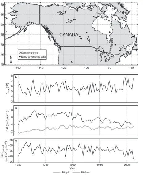
Fig. 2. annual values and

temporal trends of the calculated rates of pho-tosynthesis (expressed as Gross ecosystem exchange, Gee), the Basal area increment (Bai) and the measured climatic variables. (A) mean annual average maximum temperature averaged from the nine sites; (B) mean basal area increment (Bai) from

Pinus (Baipb) and Picea

(Baipm); (C) mean calcu-lated annual Gee.

Fig. 1. map of tree-ring

sampling sites and eddy-covariance data utilized.

3 4 5 6 7 8 Tma x (°C) A B 2 4 6 8 BAI (cm 2 year –1) 1920 1940 1960 1980 2000 –75 –70 –65 –60 –55 C GE Eannual (mol m –2 year –1) Year BAIpb BAIpm

0.5 1.0 1.5 2.0 BAI es t (cm 2 year –1) A 0 50 100 150 200 250 0.4 0.6 0.8 1.0 1.2 1.4 Age (years) BAI es t (cm 2 year –1) B

Kairiukstis 1990). Here, we analyzed the response of growth to ecosystem productivity at each of the nine sites separately.

Physiological covariates estimated from models calibrated with eddy-covariance data

We calculated time series of ecosystem produc-tivity for each site using a photosynthesis model fed with local climate data obtained from Natural Resources Canada (Régnière and Saint-Amant 2008) for the nine sites studied. First, to calibrate the model we used integrated eddy-covariance gap-filled half-hourly carbon flux data coming from the four mature black spruce or jack pine forests included in the Fluxnet-Canada Research Network (http://fluxnet.ccrp.ec.gc.ca/e_about. htm) (Table 2 and Fig. 1). Daily flux data from the four forests were calculated from the half-hourly flux measurements and ecosystem carbon data were used to calibrate daily the model from Gea-Izquierdo et al. (2010, Appendix) based on Mäkelä et al. (1996, 2004). In this big-leaf model, stand gross ecosystem exchange (GEE, in mol CO₂ m–2 _day–1_{) was estimated as a}

func-tion of atmospheric CO₂ concentration, photo-synthetically active radiation, water vapor

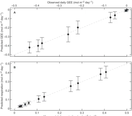
pres-sure deficit and air temperature. In the model, ecosystem respiration (R_eco) and net ecosystem exchange (NEE) were calculated as NEE = R_eco – GEE. The model provided excellent fit to the four individual flux data sets (Efficiency, EF > 0.94 see Eq. 1 below for the meaning of EF) and also when fitted to the four sites together (EF = 0.97 for daily GEE and EF = 0.91 for daily res-piration). Therefore, we fitted one single model to estimate carbon fluxes for all species and sites (Table 3 and Fig. 4; Gea-Izquierdo et al. 2010). Throughout the text, negative values of GEE and NEE correspond to a flux from the atmosphere to the land surface, i.e. GEE in all cases and NEE when photosynthesis exceeds respiration.

Once calibrated, the model was used to pro-duce daily estimates of gross and net ecosystem productivity for the nine sites along the climatic gradient and these estimates were included as covariates in the low and high-frequency analy-ses. From the daily estimates calculated for the nine sites using the model, we obtained time series of monthly, seasonal and annual ecosystem productivity, to compare with growth indices. The following flux estimates (both year t and year t – 1) were evaluated in the I_BAI analyses: (i) annual GEE, NEE, and R_eco; (ii) spring GEE, NEE, R_eco (from April, May, June, which coin-cides with the annual maximum); (iii) growing

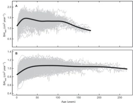
Fig. 3.

variance-stabi-lized Basal area incre-ments (Baiest) with spline

fitted (150 and 250 years respectively for jack pine and black spruce) rep-resenting the average annual growth used to detrend data in IBai: (A) Pinus banksiana and (B) Picea mariana.

season NEE, GEE and R_eco (April–September); (iv) the same for summer (June–August). The model estimates photosynthesis per ground unit area (m2_{) of closed stands. We assumed that stand}

conditions (i.e. leaf area index and closed cano-pies) would remain unchanged along time and among sites. Later in the discussion we describe possible biases which could have arrived had we applied the same analysis to open stands or to stands with variable canopy conditions.

Statistical analyses

First, to analyze the differences between mean site responses (I_BAI, low-frequency) to physi-ological covariates we used linear mixed models including a random intercept for site (Verbeke and Mohlenberghs 2000). We studied the rela-tionship between I_BAI as the dependent vari-able and physiological covariates on a single fit including all sites together. Serial correlation in the time series was taken into account by including a first auto-regressive, AR[1], vari-ance-covariance error structure to each site sub-matrix. To compare models including GEE as covariate with those including GEE2 _(quadratic

relationship) we used Akaike’s Information Cri-terion (AIC) and the model minimizing AIC was considered to be the best (Burnham & Anderson 2004). Model performance was evaluated using the model efficiency (EF):

(1) where n is the number of observations, k is the number of parameters, y_i is the ith value of measured variable y, is the predicted value, and is the mean of the measured variable). We used partitioning of variance to discuss the influence of each covariate (random and fixed) on the final model, which was calculated assum-ing that total variance equaled the sum of the individual variances of the different covariates within the linear models fitted. Secondly, for the high-frequency analysis, I_RW was compared separately for each of the nine sites with monthly estimates of the covariate explaining most

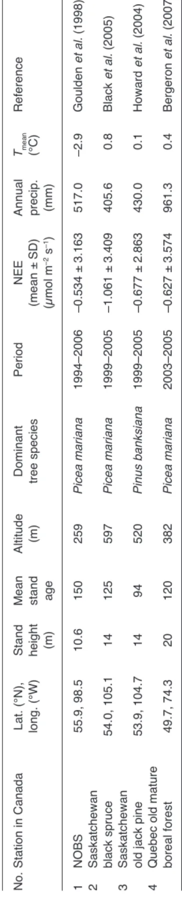
vari-Table 2

. c

haracteristics of eddy-covariance data sets used.

no. s tation in canada lat. (° n), stand m ean altitude Dominant Period nee annual Tmean reference long. (°W) height stand (m) tree species (mean ± sD) precip. (° c) (m) age (µmol m –2 s –1) (mm) 1 no Bs 55.9, 98.5 10.6 150 259 Picea mariana 1994–2006 –0.534 ± 3.163 517.0 –2.9 Goulden et al. (1998) 2 s

askatchewan _{black spruce}

54.0, 105.1 14 125 597 Picea mariana 1999–2005 –1.061 ± 3.409 405.6 0.8 Black et al. (2005) 3 s

askatchewan _{old jack pine}

53.9, 104.7 14 94 520 Pinus banksiana 1999–2005 –0.677 ± 2.863 430.0 0.1 howard et al. (2004) 4

Quebec old mature boreal forest

49.7, 74.3 20 120 382 Picea mariana 2003–2005 –0.627 ± 3.574 961.3 0.4 Bergeron et al. (2007)

ance in the I_BAI analyses. To study the linear rela-tionship between pair of variables we calculated Pearson’s correlation coefficients (r_P) (Cook and Kairiukstis 1990).

Results

Long-term growth and productivity along the latitudinal gradient

NEE and GEE variables decreased with increas-ing latitude together with mean annual tempera-ture and precipitation (Fig. 5; Huang et al. 2010). The mean BAI of both pine and spruce varied with age, in time along the 1900s and also at different sites (Figs. 2–4). There was a decrease

of mean annual growth with latitude in pine (Spearman’s correlation: r_S = –0.867, p = 0.004), but not in spruce (Spearman’s correlation: p = 0.291; Fig. 5). The ecology and growth response to climate along the gradient differed between species, thus we analyzed the two species sepa-rately. Pearson’s correlations between _BAI and annual estimates of components of ecosystem productivity (i.e. NEE, R_eco, GEE) were slightly higher than those between _BAI and summer or seasonal productivity, and correlations between

I_BAI and seasonal and annual GEE and NEE were almost identical (Table 4). For this reason, here-after we only report results using GEE covariates quoted as productivity.

High photosynthetic productivity enhanced tree growth (Table 5) and the relationship

Table 3. Best-fit model results for mean daily GEE model used to calculate ecosystem productivity series

(Appen-dix). EF = efficiency (see Eq. 1 and definition in the text).

observations τ δ αmax b Ts Bias rmse eF

(days) (µmol m–2 _s–1_{) (mol m}–2 _day–1_{) (°c) (mol m}–2 _day–1₎

10545 2.701 7.603 0.0016 –0.261 8.647 –0.001 0.032 0.967 –0.5 –0.4 –0.3 –0.2 –0.1 0

–0.5 –0.4 Observed daily GEE (mol m–0.3 –0.2 –0.1 0

–2 _day–1₎

A

Predicted GEE (mol

m –2 da y –1) 0 0.1 0.2 0.3 0.4 0.5 0 0.1 0.2 0.3 0.4 0.5 B

Measured daily respiration (mol m–2 _day–1₎

Predicted respiration (mol

m

–2 da

y

–1)

Fig. 4. residuals of

the fitted flux model expressed as monthly integrals of carbon flux: (A) Gee, (B) ecosystem respiration. Bars corre-spond to one standard deviation of the mean.

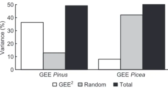
between annual productivity and growth was quadratic for both species (AIC of the model as in Table 5 using GEE as covariate instead of GEE2 _{was 11.7 units greater for pine and 13.5}

units for spruce). However the contribution of random effects in the I_BAI model reflected mean differences in radial growth between sites and showed that in the low-frequency analysis the variability of annual growth explained by pro-ductivity was reduced for spruce (Fig. 6). The

importance of random effects was much greater in the spruce model, where the fixed effects were explaining a very small part of the total variance (Table 5 and Fig. 6). As seen in Table 6 the performance of the I_BAI model had not been good if analyzed site-wise because this analy-sis neglected the high-frequency local responses to ecosystem productivity, which we analyze below. Latitude (°N) 0 2 4 6 8 10 12 BAI (cm 2 year –1) BAIpb BAIpm Latitude (°N) GEEannua l (mol m –2 year –1 ) 46 47 48 49 50 51 52 53 54 46 47 48 49 50 51 52 53 54 –80 –70 –60 –50

Fig. 5. mean Basal area

increment (Bai) of the two species analyzed and simulated mean annual Gee (grey bars, above) at the nine sites. Dashed black lines correspond to black spruce (Baipm) whereas solid black lines to jack pine (Baipb). Bars represent standard devia-tions.

Table 4. Pearson’s correlations (rP) between growth index from the low-frequency analyses (IBai) and co2 fluxes

(Gee, nee, Reco) for Pinus and Picea.

Geeannual Geeanual(t – 1) Geeseason Geespring Geesummer neeannual Reco_annual IBai Pinus –0.626 –0.614 –0.623 –0.583 –0.623 –0.625 0.624 IBai Picea –0.275 –0.263 –0.250 –0.255 –0.265 –0.274 0.264

Table 5. model results: the model for site i is: IBaii = (µ + ai) + βGee2 + εi, with ai being a random site effect, εi the

random error; µ a common intercept for the whole population and β a fixed coefficient for GEE2 _{(the quadratic}

func-tion of GEE). GEE = annual GEE; EF = efficiency calculated including the fixed and random site effects (Eq. 1); SE = standard error; AR[1] = parameter estimate of first order autoregression used in the variance-covariance structure for the error.

Gee model Parameter (covariate) estimate se eF

Pinus banksiana Fixed effect estimates µ –0.0599 0.0325 49.18

β (Gee2_{) 5.61 ¥ 10}–07 _{1.01 ¥ 10}–10

covariance estimates random intercept (site) 0.0058 0.0041

ar[1] 0.8931 0.0023

Picea mariana Fixed effect estimates µ 0.03113 0.0171 50.08

β (Gee2_{) 6.14 ¥ 10}–8 _{1.00 ¥ 10}–10

covariance estimates random intercept (site) 0.0018 0.0013

Local responses to short-term variations in productivity

Results from the high (I_RW) frequency analysis were different from those of the low-frequency (I_BAI) analysis (Fig. 7). Differences between spe-cies in correlation values between monthly-sim-ulated productivity and I_RW were smaller than those in the low-frequency I_BAI analyses (Fig. 7). Yet linear correlation coefficients between covariates and I_RW for pine were still generally greater than those for spruce (Fig. 7). In pine, growth of stands located more to the south (lati-tudes 46°–50°) responded to photosynthesis ear-lier in spring (particularly at year t) while trees from northern stands responded later in summer (Fig. 7A). The positive response of growth to productivity in black spruce was more homo-geneous along the gradient in spring, and the delay in the response with latitude was less evi-dent, particularly in the current year (Fig. 7B). Growth of spruce at low latitudes exhibited a stronger negative response to high productivity in summer of the current year. In contrast, the effect of high productivity in the summer was positive for growth at the highest latitudes for the same period. These effects in summer were detectable for both species also for the previ-ous year. In pine there was a strong relationship between growth and productivity of the previous year, with some differences between latitudes.

Discussion

Process-based growth models generally contain sets of equations of photosynthetic production and respiration, as well as rules of how this photosynthetic production is allocated to dif-ferent plant organs. In the present paper, we estimated tree-ring width at different temporal scales as a direct function of photosynthetic production. The proposed approach is a modi-fication to that in Berninger et al. (2004) who presented relationships between leaf-level pho-tosynthesis and growth of Scots pine and similar to that in Foster and Leblanc (1993) or Federer

et al. (1989). Detailed ecophysiological growth

models require knowledge of stand structure and its changes over time (Berninger et al. 2004).

This information is, however, rarely available. Permanent sample plots are usually measured only every five years or even less frequently and reconstruction of tree growth with a high tem-poral resolution depends largely on tree rings. Photosynthetic production depends on the cli-mate and properties of the plant canopy (e.g. Le Roux et al. 2001). The present modeling approach keeps the canopy characteristics fixed and focuses on the estimation of the climatic effects on photosynthesis as e.g. in Mäkelä et

al. (2008a) or Gea-Izquierdo et al. (2010). We

acknowledge that there are changes in forest pro-ductivity associated with changes in the physi-ological properties of leaves (Kaufmann et al. 2004) and forests in more productive areas or during more productive periods would prob-ably have higher leaf area index (LAI), hence higher photosynthetic production. However, we

GEE Pinus GEE Picea

GEE2 _{Random Total}

Variance (% ) 0 10 20 30 40 50

Fig. 6. Partition of variability contribution (%) of fixed

effects and random effects for the Gee jack pine model (‘Gee Pinus’ in the x-axis) and Gee spruce model (‘Gee Picea’ in the x-axis) expressed as percentages of efficiencies (EF) of those covariates and total effi-ciencies shown in table 5.

Table 6. Contribution of individual fixed effect (GEE2₎

to the explained variability for Pinus banksiana and

Picea mariana if calculated by site using the overall IBai

models in table 5. all values are percentages. site Pinus banksiana Picea mariana

46° 0.05 0.56 47° 0.04 2.08 48° 0.47 0.68 49° 1.36 2.48 50° 0.08 0.38 51° 0.05 0.31 52° 1.01 1.86 53° 7.14 0.44 54° 1.72 1.37 mean (sD) 1.32 (2.27) 1.13 (0.83)

Fig. 7. Bootstrap

correla-tions between individually detrended rW (IrW) data

and monthly Gee (from april to november year t – 1, and from march to sep-tember year t): (A) Pinus

banksiana Gee, (B) Picea mariana Gee. White dots

indicate significant correla-tions. note that high nega-tive Gee values indicate the forest being a carbon sink hence negative cor-relations between growth and Gee express that greater photosynthesis at a specific period increases growth. the grey scale represents Pearson’s cor-relations ranging between –0.4 and 0.5.

do not think that this would change qualitatively our results because annual fluctuations of tree growth are directly linked to lagged GEE (i.e. through and autoregressive model). Hence simi-lar relationships between photosynthetic produc-tion and tree ring width would be maintained, particularly when studying growth anomalies in the high-frequency analysis.

Time-scale, species-specific

relationships between radial growth and productivity

The relationship between ecosystem productivity

and radial growth is complex. Tree-ring growth reflected both long- and short-term variations in site productivity but not equally for all sites and species. The long-term mean gross ecosys-tem exchange was well related only to annual radial growth of one boreal evergreen coniferous species along a latitudinal gradient, jack pine, whereas the correlation with black spruce was very weak. In the short-term, annual anomalies of tree growth were well related to simulated productivity at all sites and for both species. The fit of this relationship (absolute maximum cor-relation values around 0.4; Fig. 7) was similar to that found for empirical dendroecological models using temperature or growing degree days as the

main driver (Hofgaard et al. 1999; Huang et al. 2010). Results from tree-ring empirical models are often similar to results from process-based approaches (e.g. Berninger et al. 2004, Anchu-kaitis et al. 2006, Evans et al. 2006, Shi et al. 2008). The reason for the similar performance of photosynthesis based and climate based empirical models could be that the non-linear relationship between temperature (in our boreal stands) and photosynthetic production converged to linear when analyzed in long time periods.

The differences in the time scale of the rela-tionship between growth and productivity could explain why models of ecosystem productivity and tree growth seem to operate on different pro-cesses. Ecosystem productivity in boreal forests where drought is usually not limiting seems to depend largely on the length of the photosynthet-ically active period (Suni et al. 2003a, 2003b) which usually starts in April or May. Annual tree diameter growth anomalies, on the other hand, seem to depend on summer temperatures (Kirdy-anov et al. 2003, D’Arrigo et al. 2004, Vag(Kirdy-anov

et al. 2006) and growth can correlate quite well

with temperatures during short periods (Kirdy-anov et al. 2003). Cambial activity is tempera-ture-dependent and varies at different sites and for different species, but higher temperatures are required for xylem cell division than for photo-synthesis in the leaves (Körner 1998, Suni et al. 2003b, Rossi et al. 2011). Therefore, time-scale dependent relationships exist between net carbon fixation and growth and the relationship between these two variables is not a fixed ratio (Luys-saert et al. 2007, Granier et al. 2008, Zweifel et

al. 2010). Trees in boreal forests are considered

to use the period of maximum productivity to allocate carbon to the stem for growth, and this period is delayed in summer with increasing latitude (Kirdyanov et al. 2003). After summer, during those months prior to the dormant period, the trees store carbohydrates for next year’s growth (Granier et al. 2008) and year-to-year variations in productivity could be averaged out by changes in carbohydrates reserve or alloca-tion, which results in more diffuse and difficult to detect relationships between GEE and growth.

Our results agree with those of authors show-ing a correlation between the high-frequency of growth and photosynthesis (Berninger et al. 2004,

Hari and Nöjd, 2009, Zweifel et al. 2010), but different relationships were found for the differ-ent sites. Allocation of carbohydrates was the most likely mechanism explaining differences in the growth response between sites and species. Rocha et al. (2006) explained the lack of cor-relation between measured GEE and ring width on a black spruce site in northern Canada by interannual differences in allocation. Granier et

al. (2008) suggested that carbon allocation from

photosynthesis is constant during the period when cambium is active in Fagus sylvatica but car-bohydrate allocation is a complex phenomenon that is likely to vary with species and also other factors such as climate, soil or even competition (Gough et al. 2002, Rocha et al. 2006). Further-more, there is evidence for systematic changes in allocation with varying temperature and an inter-action of precipitation with temperature along climatic gradients (Vogel et al. 2008). In practice this means that the short-term tree growth may be decoupled from photosynthesis and that trees may modify their growth in response to long-term changes in photosynthetic production (D’Arrigo

et al. 2004, Kaufmann et al. 2004). Zweifel et al.

(2010) showed the potential complexity of the relationship between growth and photosynthesis and found a strong correlation between cambial activity and GEE which was a function of the time scale, as was also found by Granier et al. (2008). Stronger correlations can be expected at single sites where both flux and growth are measured (e.g. Zweifel et al. 2010) as compared with cases where productivity needs to be simulated along climatic gradients, like we did here.

Other factors precluding a general direct relationship between growth and

productivity

Stand-related factors such as stand density, char-acteristics of tree individuals or microenviron-mental variability could also modify the rela-tionship between photosynthesis and growth. To minimize the influence of competition and tree dendrometric features at the different sites we selected mature stands with closed canopies, similar to those used to calibrate the photo-synthesis model. However, selection of only

dominant trees, as done classically in many dendrochronological studies, may bias estimated stand growth and its relationship with stand pho-tosynthesis. We believe that the influence of this was minimal at the sampled sites because stands were post-fire, closed and structurally homoge-neous. The differences among sites and between species in our results could also be explained by non-climatic factors such as nitrogen avail-ability (Mäkelä et al. 2008b), insect infestation in spruce (Bouchard et al. 2005), different litter decomposition and nitrogen mineralization rates (Bergh et al. 1999, Berninger et al. 2004) or the effect of the humus layer on a differential response to drought (Drobyshev et al. 2010). Only jack pine decreased its mean radial growth with increasing latitude, hence site temperature and productivity, indicating that climate con-trolled most of what foresters call ‘site quality’ for jack pine. For spruce, differences between sites in average growth seemed to be determined by non-climatic factors. Black spruce occupies many different environments in the boreal region of North America, but is not very competitive on eutrophic sites. Those sites occupied by black spruce change along the gradient studied: in the North it is a generalist growing on all types of sites (including good sites), whereas in the south it is restricted to poor sites (Burns and Honkala 1990, Hofgaard et al. 1999). This shift of the realized niche of black spruce could explain its low response to changes in average simulated GEE along the gradient.

NEE was not better correlated with radial growth than GEE probably due to the fact that the fraction of autotrophic to heterotrophic respi-ration was highly variable between sites (Lloyd and Taylor 1994, Xu et al. 2004). Estimated respiration was closely related to NEE and GEE estimates, but its correlation with growth was weaker than with GEE, contrary to Rocha et

al. (2006) but in accordance with Zweifel et al.

(2010). However, according to the literature, respiration is only a minor component of interan-nual variability in carbon fluxes in boreal forests (Suni et al. 2003a, 2003b) while respiration seems to be a major determinant of inter-site variability of net productivity (Valentini et al. 2000, Luyssaert et al. 2007). It could be that a varying proportion of GEE is fixed by

veg-etation in the understory (Knorre et al. 2006). It could be argued that our GEE model was not applicable given the distance between our sites and three of the flux towers used for the model calibration. The southern stands were in more temperate climate than the eddy-covar-iance sites, and we found a different response to GEE in summer (particularly of the previous year) for southern sites as compared with that for sites located more to the north. Therefore, it is possible that the photosynthetic production at these sites was more limited by drought than in our calibration data set, and that we overesti-mated photosynthetic production during summer in the southernmost stands. This would explain the inverse relationship between summer pho-tosynthetic production and growth (expressed as a positive relationship in Fig. 7) for southern sites. Nevertheless in the eddy-covariance-based analysis of Gea-Izquierdo et al. (2010) drought did not appear to affect the estimated GEE at any site with mean temperature below 2.5 °C, like those included in our gradient (Huang et al. 2010). In that paper, the authors tried to incor-porate the effects of drought into the model, but concluded that the effect of drought was minor. Additionally the model had a good fit to conifer-ous GEE data regardless of species or geographi-cal locations, and the same type of model with small changes in parameters could be used for different sites along a climatic gradient including sites below 46°N (Gea-Izquierdo et al. 2010). The reason for the better fit for jack pine was not in the photosynthesis model since the photosyn-thesis model was calibrated using mostly black-spruce stands. We therefore believe that using a single GEE model on the geographical gradient studied did not lead to biased results that would compromise our conclusions.

In boreal ecosystems, temperature is gener-ally the strongest driver of photosynthesis and growth and recent decades warming mostly resulted on an increase in photosynthetic activity (Myneni et al. 1997), as reflected by our produc-tivity estimates. Pine growth showed a time trend that we interpreted as an age effect but could also be interpreted as a growth decline reflecting a drought effect in recent years (e.g. Hofgaard et

al. 1999, Dulamsuren et al. 2010). However,

53°N (the second northernmost site) and our high-frequency analysis suggests greater water limitations in spruce than in pine. We would expect (if any) water stress limitation to be more widespread in southern stands (Hofgaard

et al. 1999) and in any case, any existing age

trend did not affect our analysis because growth data were standardized using dendrochronologi-cal methods. We analyzed high-frequency and low-frequency responses separately in our paper. The high-frequency is likely to be of secondary importance in long-term growth trends under climate warming and also in terms of productiv-ity. We still do not understand how long-term changes in net productivity and photosynthesis allocation to stem growth will interact. Growth changes in the future may be, therefore, different than just changes in photosynthetic production.

Conclusions

The relationships between estimated ecosystem productivity and tree-ring width were different for the two species depending on the tempo-ral scale analyzed and along the studied cli-matic gradient, probably reflecting differences in phenology and species-specific carbon allo-cation strategies. The year-to-year response of growth (annual anomalies from the site mean) was enhanced by ecosystem productivity in both species whereas the long-term relationship of average tree annual growth with ecosystem pro-ductivity showed a good agreement with over-all photosynthesis only for jack pine. Proba-bly long-term variations in net photosynthesis change the response of growth to climate, which also depends on non-climatic factors. There is a considerable potential to understand these vari-ations and use tree-ring growth as a proxy for ecosystem productivity but this would require a deeper understanding of the possibly interfering factors, in particular of interannual variations in carbohydrate allocation.

Acknowledgements: We are most indebted to Fluxnet Canada,

especially Hank Margolis, Andy T. Black and Allison Dunn for sharing the eddy-covariance data to calibrate the model. This contribution was partly funded by a NSERC strategic grant hold by Y.B. and F.B.

References

Anchukaitis K.J., Evans M.N., Kaplan A., Vaganov E.A., Hughes M.K., Grissino-Mayer H.D. & Cane M.A. 2006. Forward modeling of regional scale tree-ring patterns in the outheastern United States and the recent influ-ence of summer drought. Geophys. Res. Let. 33(4), doi:10.1029/2005gl025050.

Baldocchi D.D. 2003. Assessing the eddy covariance tech-nique for evaluating carbon dioxide exchange rates of ecosystems: past, present and future. Global Change

Biol. 9: 479–492.

Bergeron O., Margolis H.A., Black T.A., Coursolle C., Dunn A.L., Barr A.G. & Wofsy S.C. 2007. Comparison of carbon dioxide fluxes over three boreal black spruce for-ests in Canada. Global Change Biol. 13: 89–107. Bergh J., Linder S., Lundmark T. & Elfving B. 1999. The

effect of water and nutrient availability on the productiv-ity of Norway spruce in northern and southern Sweden.

Forest Ecol. Manage. 119: 51–62.

Berninger F., Hari P., Nikinmaa E., Lindholm M. & Meriläi-nen J. 2004. Use of modeled photosynthesis and decom-position to describe tree growth at the northern tree line.

Tree Physiol. 24: 193–204.

Black T.A., Gaumont-Guay D., Jassal R.S., Amiro B.D., Jarvis P.G., Gower S.T. & Kelliher F.M. 2005. Measure-ment of CO2 exchange between boreal forest and the

atmosphere. In: Griffiths H. & Jarvis P.J. (eds.), The

carbon balance of forest biomes, Taylor and Francis,

NY, pp. 151–186.

Boisvenue C. & Running S.W. 2006. Impacts of climate change on natural forest productivity — evidence since the middle of the 20th century. Global Change Biol. 12: 862–882.

Bouchard M., Kneeshaw D. & Bergeron Y. 2005 Mortality and stand renewal patterns following the last spruce-budworm outbreak in mixed forests of western Quebec.

Forest Ecol. Manage. 204: 297–313.

Burnham K.P., Anderson D.R., 2004. Multimodel infer-ence — understanding AIC and BIC in model selection.

Sociological Methods & Research 33: 261–304.

Burns M. & Honkala B.H. 1990. Silvics of North America: 1.

Conifers. Agriculture Handbook 654, U.S. Department

of Agriculture, Forest Service, Washington, DC. Cook E.R. & Peters K. 1997. Calculating unbiased tree-ring

indices for the study of climatic and environmental change. Holocene 7: 361–370.

Cook E.R. & Kairiukstis L.A. (eds.) 1990. Methods of

den-drochronology. Applications in the environmental sci-ences. Kluwer, Dordrecht.

D’Arrigo R.D., Kaufmann R.K., Davi N., Jacoby G.C., Laskowski C., Myneni R.B. & Cherubini P. 2004. Thresh-olds for warming-induced growth decline at elevational tree line in the Yukon Territory, Canada. Glob.

Biogeo-chem. Cy. 18, GB3021, doi:10.1029/2004GB002249.

Drew D.M., Downes G.M. & Battaglia M. 2010. CAM-BIUM, a process-based model of daily xylem develop-ment in Eucalyptus. J. Theor. Biol. 264: 395–406. Drobyshev I., Simard M., Bergeron Y. & Hofgaard A. 2010.

Does soil organic layer thickness affect climate-growth relationships in the black spruce boreal ecosystem?

Eco-systems 13: 556–574.

Dulamsuren C., Hauck M. & Leuschner C. 2010. Recent drought stress leads to growth reductions in Larix

sibir-ica in the western Khentey, Mongolia. Global Change Biol 16: 3024–3035.

Ehman J.L., Schmid H.P., Grimmond C.S.B., Randolph J.C., Hanson P.J., Wayson C.A. & Cropley F.D. 2002. An initial intercomparison of micrometeorological and ecological inventory estimates of carbon exchange in a mid-latitude deciduous forest. Global Change Biol. 8: 575–589.

Esper J., Cook E.R., Krusic P.J., Peters K. & Schweingru-ber F.H. 2003. Tests of the RCS method for preserving low-frequency variability in long tree-ring chronologies.

Tree-Ring Res. 59: 81–98.

Evans M.N., Reichert B.K., Kaplan A., Anchukaitis K.J., Vaganov E.A., Hughes M.K. & Cane M.A. 2006. A forward modeling approach to paleoclimatic interpreta-tion of tree-ring data. J. Geophys. Res.-Biogeo. 111, doi:10.1029/2006jg000166.

Federer C.A., Tritton L.M., Hornbeck J.W. & Smith R.B. 1989. Physiologically based dendroclimate models for effects of weather on red spruce basal-area growth. Agr.

Forest Meteorol. 46: 159–172.

Foster J.R. & Leblanc D.C. 1993. A physiological approach to dendroclimatic modeling of oak radial growth in the Midwestern United-States. Can. J. Forest Res. 23: 783–798.

Gea-Izquierdo G., Mäkelä A., Margolis H., Bergeron Y., Black A.T., Dunn A., Hadley J., Paw U.K.T., Falk M., Wharton S., Monson R., Hollinger D.Y., Laurila T., Aurela M., McCaughey H., Bourque C., Vesala T. & Berninger F. 2010. Modeling acclimation of photosyn-thesis to temperature in evergreen boreal conifer forests.

New Phytol. 188: 175–186.

Girardin M.P., Raulier F., Bernier P.Y. & Tardif J.C. 2008. Response of tree growth to a changing climate in boreal central Canada: A comparison of empirical, process-based, and hybrid modelling approaches. Ecol. Model. 213: 209–228.

Gough C.M., Vogel C.S., Schmid H.P., Su H.B. & Curtis P.S. 2008. Multi-year convergence of biometric and mete-orological estimates of forest carbon storage. Agr. Forest

Meteorol. 148: 158–170.

Goulden M.L., Winston G.C., McMillan A.M.S., Litvak M.E., Read E.L., Rocha A.V. & Rob Elliot J. 2006. An eddy covariance mesonet to measure the effect of forest age on land-atmosphere exchange. Global Change Biol. 12: 2146–2162.

Granier A., Breda N., Longdoz B., Gross P. & Ngao J. 2008. Ten years of fluxes and stand growth in a young beech forest at Hesse, north-eastern France. Ann. Forest Sci. 64: 704.

Hari P. & Nöjd P. 2009. The effect of temperature and PAR on the annual photosynthetic production of Scots pine in northern Finland during 1906–2002. Boreal Env. Res. 14: 5–18.

Hofgaard A., Tardif J. & Bergeron Y. 1999. Dendroclimatic

response of Picea mariana and Pinus banksiana along a latitudinal gradient in the eastern Canadian boreal forest.

Can. J. Forest Res. 29: 1333–1346.

Howard E.A., Gower S.T., Foley J.A. & Kucharik C.J. 2004. Effects of logging on carbon dynamics of a jack pine forest in Saskatchewan, Canada. Global Change Biol. 10 (8): 1267–1284.

Huang J.G., Tardif J.C., Bergeron Y., Denneler B., Berninger F. & Girardin M.P. 2010. Radial growth response of four dominant boreal tree species to climate along a latitudinal gradient in the eastern Canadian boreal forest.

Global Change Biol. 16: 711–731.

Kaufmann R.K., D’Arrigo R.D., Laskowski C., Myneni R.B., Zhou L. & Davi N.K. 2004. The effect of growing season and summer greenness on northern forests.

Geo-phys. Res. Lett. 31. doi 10.1029/2004gl019608.

Kirdyanov A., Hughes M., Vaganov E., Schweingruber F. & Silkin P. 2003. The importance of early summer tem-perature and date of snow melt for tree growth in the Siberian Subarctic. Trees-Struct. Funct. 17: 61–69. Knorre A., Kirdyanov A. & Vaganov E. 2006. Climatically

induced interannual variability in aboveground produc-tion in forest-tundra and northern taiga of central Sibe-ria. Oecologia 147: 86–95.

Kramer K., Leinonen I., Bartelink H.H., Berbigier P., Borghetti M., Bernhofer C.H., Cienciala E., Dolman A.J., Froer O., Gracia C.A., Granier A., Grunwald T., Hari P., Jans W., Kellomaki S., Loustau D., Magnani F., Markkanen T., Matteucci G., Mohren G.M.J., Moors E., Nissinen A., Peltola H., Sabate S., Sanchez A., Sontag M., Valentini R. & Vesala T. 2002. Evaluation of six pro-cess-based forest growth models using eddy-covariance measurements of CO2 and H2O fluxes at six forest sites

in Europe. Global Change Biol. 8: 213–230.

Körner C. 1998. A re-assessment of high elevation tree-line positions and their explanation. Oecologia 115: 445–459.

Le Roux X., Lacointe A., Escobar-Gutierrez A. & Le Dizes S. 2001. Carbon-based models of individual tree growth: A critical appraisal. Ann. Forest Sci. 58: 469–506. Lloyd J. & Taylor J.A. 1994. On the temperature dependence

of soil respiration. Funct. Ecol. 8: 315–323.

Luyssaert S., Inglima I., Jung M., Richardson A.D., Reich-stein M., Papale D., Piao S.L., Schulzes E.D., Wingate L., Matteucci G., Aragao L., Aubinet M., Beers C., Bernhoffer C., Black K.G., Bonal D., Bonnefond J.M., Chambers J., Ciais P., Cook B., Davis K.J., Dolman A.J., Gielen B., Goulden M., Grace J., Granier A., Grelle A., Griffis T., Gruenwald T., Guidolotti G., Hanson P.J., Harding R., Hollinger D.Y., Hutyra L.R., Kolar P., Kruijt B., Kutsch W., Lagergren F., Laurila T., Law B.E., Le Maire G., Lindroth A., Loustau D., Malhi Y., Mateus J., Migliavacca M., Misson L., Montagnani L., Moncrieff J., Moors E., Munger J.W., Nikinmaa E., Ollinger S.V., Pita G., Rebmann C., Roupsard O., Saigusa N., Sanz M.J., Seufert G., Sierra C., Smith M.L., Tang J., Val-entini R., Vesala T. & Janssens I.A. 2007. CO2 balance

of boreal, temperate, and tropical forests derived from a global database. Global Change Biol. 13: 2509–2537. Mäkelä A., Berninger F. & Hari P. 1996. Optimal control of

gas exchange during drought: theoretical analysis. Ann.

Bot. London 77: 461–467.

Mäkelä A., Hari P., Berninger F., Hänninen H. & Nikinmaa E. 2004. Acclimation of photosynthetic capacity in Scots pine to the annual cycle of temperature. Tree Physiol. 24: 369–376.

Mäkelä A., Pulkkinen M., Kolari P., Lagergren F., Berbigier P., Lindroth A., Loustau D., Nikinmaa E., Vesala T. & Hari P. 2008a. Developing an empirical model of stand GPP with the LUE approach: analysis of eddy covari-ance data at five contrasting conifer sites in Europe.

Global Change Biol. 14: 92–108.

Mäkelä A., Valentine H.T. & Helmisaari H.S. 2008b. Opti-mal co-allocation of carbon and nitrogen in a forest stand at steady state. New Phytol. 180: 114–123. Misson L. 2004. MAIDEN: a model for analyzing ecosystem

processes in dendroecology. Can. J. Forest Res. 34: 874–887.

Myneni R.B., Keeling C.D., Tucker C.J., Asrar G. & Nemani R.R. 1997. Increased plant growth in the northern lati-tudes from 1981 to 1991. Nature 386: 698–702. Ohtsuka T., Saigusa N. & Koizumi H. 2009. On linking

mul-tiyear biometric measurements of tree growth with eddy covariance-based net ecosystem production. Global

Change Biol. 15: 1015–1024.

Rathgeber C., Nicault A., Kaplan J.O. & Guiot J. 2003. Using a biogeochemistry model in simulating forests produc-tivity responses to climatic change and [CO₂] increase: example of Pinus halepensis in Provence (south-east France). Ecol Model. 166: 239–255.

Régnière J. & Saint-Amant R. 2008. BioSIM 9 — user’s

manual. Rep. LAU-X-134E, Natural Resources Canada,

Canadian Forest Service, Laurentian Forestry Centre, Quebec, QC.

Rocha A.V., Goulden M.L., Dunn A.L. & Wofsy S.C. 2006. On linking interannual tree ring variability with observa-tions of whole-forest CO₂ flux. Global Change Biol. 12: 1378–1389.

Rossi S., Morin H., Deslauriers A. & Plourde P.Y. 2011. Pre-dicting xylem phenology in black spruce under climate warming. Global Change Biol. 17: 614–625.

Running S.W. 1994 Testing FOREST-BGC ecosystem pro-cess simulations across a climatic gradient in Oregon.

Ecol. Appl. 4: 238–247.

Shi J.F., Liu Y., Vaganov E.A., Li J. & Cai A. 2008. Statisti-cal and process-based modeling analyses of tree growth response to climate in semi-arid area of north central China: a case study of Pinus tabulaeformis. J. Geophys.

Res. 113, G01026, doi:10.1029/2007JG000547

Suni T., Berninger F., Markkanen T., Keronen P., Rannik Ü. & Vesala T. 2003a. Interannual variability of growing-sea-son timing, length, and CO₂ exchange in a boreal forest.

J. Geophys. Res. 108: 4265, doi:10.1029/2002JD002381.

Suni T., Berninger F., Vesala, T., Markkanen T., Hari P., Mäkelä A., Ilvesniemi H., Hänninen H., Nikinmaa E., Huttula T., Laurila T., Aurela M., Grelle A., Lindroth A., Arneth A., Shibistova O. & Lloyd J. 2003b. Air tem-perature triggers the commencement of evergreen boreal forest photosynthesis in spring. Global Change Biol. 9: 1410–1426.

Vaganov E.A., Hughes M.K. & Shashkin A.V. 2006. Growth

dynamics of conifer tree rings. Springer, Berlin.

Valentini R., Matteucci G., Dolman A.J., Schulze E.D., Rebmann C., Moors E.J., Granier A., Gross P., Jensen N.O., Pilegaard K., Lindroth A., Grelle A., Bernhofer C., Grünwald T., Aubinet M., Ceulemans R., Kowalski A.S., Vesala T., Rannik Ü., Berbigier P., Loustau D., Guo-mundsson J., Thorgeirsson H., Ibrom A., Morgenstern K., Clement R., Moncrieff J., Montagnani L., Minerbi S. & Jarvis P.G. 2000. Respiration as the main determi-nant of carbon balance in European forests. Nature 404: 861–865.

Verbeke G. & Molenberghs G. 2000. Linear mixed models

for longitudinal data. Springer-Verlag, Berlin.

Vogel J.G., Bond-Lamberty B.P., Schuur E.A.G., Gower S.T., Mack M.C., O’Connell K.E.B., Valentine D.W. & Ruess R.W. 2008. Carbon allocation in boreal black spruce forests across regions varying in soil temperature and precipitation. Global Change Biol. 14: 1503–1516. Xu L., Baldocchi D.D. & Tang J. 2004. How soil moisture,

rain pulses, and growth alter the response of ecosystem respiration to temperature. Global Biogeochem. Cy. 18: 1–10.

Zweifel R., Eugster W., Etzold S., Dobbertin M., Buchmann N. & Haesler R. 2010. Link between continuous stem radius changes and net ecosystem productivity of a subalpine Norway spruce forest in the Swiss Alps. New

Phytol. 187: 819–830.

Appendix

NEE was modeled using a flux partitioning algorithm where: NEE = Reco – GEE, with GEE being

gross ecosystem exchange (photosynthesic production) and Reco being ecosystem respiration. All C

flux estimates are in mol m–2 _day–1_{. R}

eco was modeled assuming an Arrhenius type relationship with air

temperature, using the expression:

where T_air(t) is the measured temperature (°C) above the canopy and R₁₀ is the mean respiration at

10 °C. After comparing different ways of temporal fitting (monthly, every second week, annual), we decided to fit a single expression per site since the differences in the proportion of explained variance were not very large.

In the model, the gross photosynthetic rate per unit ground area A(t) (mol CO₂ m–2 _day–1_{) was}

modeled as a nonlinear function of stomatal conductance of carbon dioxide g(t) (mol CO₂ m–2 _day–1_),

photosynthetic capacity α(t) (mol CO₂ m–2 _day–1_{), and a saturation function of light intensity γ(t)}

(dimensionless):

(A2) where the stomatal conductance is expressed as:

g(t) = max{0.00001, (t)}, (A3)

with

(A4) and the light response of biochemical reactions of photosynthesis:

(A5) where C_a is the air CO₂ concentration in ppm, Q(t) is the incident photosynthetically active radiation (µmol m–2 _s–1 _{), D(t) is the water vapor pressure deficit (kPa) calculated using temperatures above the}

tree canopies, δ is the half saturation parameter of the light function (µmol m–2 _s–1_{) and λ is a model}

parameter expressing the carbon required in the long term to sustain transpiration flow (kPa). λ was set to 3000 as in Gea-Izquierdo et al. (2010).

Photosynthetic capacity α(t) was modeled as a lagged function of temperature S(t), following: with

α(t) = α_max/{1 + exp[b(S(t) – T_s)]} (A6)

and, S(t) from

(A7)

T_air(t) is the measured air temperature (°C) at time t, and α_max (mol m–2 _day–1_{), b (°C}–1_{), T}

s (°C) and

τ (days) are the model parameters: α_max is the maximum photosynthetic efficiency, which takes into

account whole canopy properties; b is the curvature of the sigmoid function and T_s is the inflection point of the sigmoid curve, i.e. the temperature at which α reaches half of α_max; and τ is the time constant of photosynthetic acclimation and indicates the time it takes for photosynthetic capacity to acclimate itself to changing temperature. All original references to the different parts of the model and a further explanation on the model can be found in Gea-Izquierdo et al. (2010).