Stochastic Metamodel for Probability of Detection Estimation of Eddy-Current Testing Problem in Random Geometric

Science Arts & Métiers (SAM)

is an open access repository that collects the work of Arts et Métiers Institute of

Technology researchers and makes it freely available over the web where possible.

This is an author-deposited version published in: https://sam.ensam.eu Handle ID: .http://hdl.handle.net/10985/16564

To cite this version :

Djamel Eddin ABDELLI, Thanh Hung NGUYEN, Stéphane CLENET, Ahmed CHERIET

-Stochastic Metamodel for Probability of Detection Estimation of Eddy-Current Testing Problem in Random Geometric - IEEE Transactions on Magnetics - Vol. 55, n°6, p.1-4 - 2019

Any correspondence concerning this service should be sent to the repository Administrator : archiveouverte@ensam.eu

Stochastic Metamodel for Probability of Detection Estimation of

Eddy Current Testing Problem in Random Geometric Problem

D. E. Abdelli

1

, T. T. Nguyen

2

, S. Clénet

2

, and A. Cheriet

1 1

LGEB, Univ. Biskra, BP 145 RP, 07000 Biskra, Algeria

2_{Univ. Lille, Centrale Lille, Arts et Métiers Paris Tech, HEI, EA 2697- L2EP –Laboratoire d'Electrotechnique et}

d'Electronique de Puissance, F-59000 Lille, France E-mail: abdelli22djamel@yahoo.com

The calculation of the Probability Of Detection (POD) in Non Destructive Eddy Current Testing requires the solution of a stochastic model requiring numerous calls of a numerical model leading to a huge computation time. To reduce this computation time, we propose in this paper to combine either the use of a stochastic metamodel and a mapping which avoids the remeshing step. The stochastic metamodel is constructed using the Least Angle Regression Method. This approach is tested on a axisymmetric problem with 6 random input paramters which shows its efficiency and its accuracy.

Index Terms— Eddy Current Testing, Finite Volume Method, Stochastic Model, Least Angle Regression Method, Probability Of Detection.

I. INTRODUCTION

owadays, non-destructive testing (NDT) is an essential element of component quality qualification. For inspecting materials and components, several methods are developed. One of these methods is the Eddy Current Method (ECT). The qualification of this process is then required. The size of defects that can be detected should be determined. In practice, it appears that imperfections on the sensors or uncertainties on the material characteristics to be inspected modify the response of the NDT device. The measurement is not deterministic and varies around a targeted value. For this reason, a statistical study must be carried out to calculate the possibility of detecting (or not) defects under different operation conditions [1-2]. A Probability Of Detection (POD) can be estimated to quantify this capability of the NDT device to detect a defect.

The ECT system can be represented by electromagnetic equations such as Maxwell's equations. The difficulty of solving these equations analytically leads to use a numerical method to construct an accurate model. In this work, the Finite Volume (FV) method has been applied. As long as the input parameters are no longer nominal values, so the numerical model FV can be represented by a stochastic system [3] with input parameter which are random.

The response of ECT system is no longer deterministic and a sampling technic like the Monte Carlo Simulation Method can be used to characterize the output and particularly to calculate the POD. A high number of calls of the numerical model FV are required. So repeating the model FV for a fairly large number of realizations is time consuming, especially when the geometry is modified because the mesh should be modified. To avoid the remeshing (RM), a geometric transformation (GT) method [4] has been used which consists in changing the coordinates of the nodes without changing their connectivity. The GT method has been used to solve an electrokinetic problem [5] and more recently a magnetoelectric problem [6]. To approximate the response of the stochastic system, a stochastic metamodel [2-3, 7] is

constructed based on a polynomial chaos expansion and the Least Angle Regression (LAR) method.

In this work the numerical POD of the defect depth is estimated using the Hit/Miss method in both methods GT and RM. To reduce the time calculation a stochastic metamodel is used in both methods (GT and RM) to approximate the responses. The two approaches are compared on a NDT stochastic example.

II. ECT AND FV MODEL

The ECT problem is modeled by the axisymmetric formulation of the magnetic vector potential " A " in the domain Ω is used as follows:

1 . j wσ , in µ   −∇  ∇ + = Ω  A A Js (1)

with w , J , s σ , and µ are the angular frequency, source

current density, electrical conductivity and magnetic permeability respectively.

N

tt rci wc

tc

σ

µ

a

Fig. 1 Coil-tube geometry [8], with rci, wc, tc are the inner radius, the width, height of the coil, tt the thickness of the tube, and the defect a (shaded area).

This ECT problem consists of a coil located in a steam generator tube with an external circumferential defect. The geometry is shown in Fig. 1.

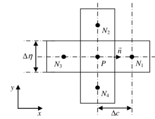
To solve Eq.1 with the FV model, we subdivide the domain into a large number of elements (triangle or quadrilateral). The integration of Eq.1 over each element (P) of the domain Ω is required as it is shows in Fig. 2.

The integration of first term of Eq.1 over the element P can be done by using the divergence theorem as in:

1 1 .( ). ( ). . 1 , i i i i s N P i i i f d c η η µ µ η µ ∆ ∇ ∇ = ∇ − = ∆ ∆

∫∫

∫

∑

r



A ds A n A A (2) where i N

A , A are the nodal magnetic vector potential of the _P nodesN (i=1:4) , P respectively, _i f are the faces with i

r n its outward normal vector , ∆c_i are the distances between the centres of N and P , _i ∆η_i are the lengths of the edges of the element. The non-orthogonal term is considered and interpolated as in [9]. We first solve the Eq.1 for the unknown potential A for all elements of the mesh and then we calculate the impedance of coil which is the quantity of interest to detect the default. It can be calculated using Faraday’s law and Stokes theorem [10] as follow:

. . j w Z d Ω = − Ω

∫

∫



s A dl J (3)

III. PROBABILITY OF DETECTION ESTIMATION

A. Empirical POD

The determination of the empirical POD requires considerable experimental measurements. A large number of samples are required to have a representative statistical population for signal of the defect. This method is time consuming and very expensive [11]. In this paper, we work with the numerical POD.

B. Numerical POD

• Monte Carlo Simulation Method (MCSM)

The Monte Carlo Simulation method [3, 12] consists in generating a sample of size which corresponds to M realizations of the input parameters, to solve M times the model and then in a postprocessing to give an estimation of the POD.

Its accuracy depends on sample size, and convergence is relatively low. Indeed, thousands of random realizations are often required to obtain a desired accuracy of the POD, which necessarily implies a high calculation time.

For the implementation of the MCSM, it is assumed that the input parameters are independent and have a uniform distribution.

• Stochastic model

As long as the calculated response of the ECT system is no longer nominal (deterministic), the notation of a random variable ( Z ) is used. So the stochastic model is given by the function:

(

, a .

)

Z = f X (4) where a is the depth of the defect (in the case without defect

a=0 and Z is denoted Z ) and X the vector a finite ₀

number of random input parameters. To alleviate the notations, we replace in the following Z = f

(

X, a

)

by

( )

Z X (or Z ). X (

{

₁, ₂,...,

}

X N X = X X X with X N the

number of input parameters) gathers the input parameters which are :σ ±10 %,µ +10 %, rci wc tc, , ±5 %, and

5%

tt± . The depths of the defect are 0.05, 0.4970 and 0.9675 mm of the thickness tube with a width of 1.5 mm. The defect is circular and coaxial with the coil.

The model Z can be replaced by an approximate model (metamodel) Zˆ = f_LAR

(

X, a

)

and is given in the following equation:

(

_{, a}

)

ˆ

(

_{, a .}

)

LAR

Z = f X ≈Z = f X (5) The metamodel will be discussed in the next section. The Monte Carlo Simulation is applied to the model Z

( )

X or

ˆ ( )

Z X in order to estimate the POD.

• Stochastic Metamodel

It is necessary to find a model faster than the FV model in order to reduce the calculation time. In this case, it may be considered to propagate the uncertainties through a metamodel constructed from Truncated Polynomial Chaos Expansion [12]. In that case, the approximation ˆ (Z X of the stochastic ) FV model Z

( )

X can be written in the form [7]:

( )

(

)

1 ˆ ( ) , out P i i i Z X α ξ X = =

∑

Ψ (6) N3 N1 N2 N4 P nr

c ∆

x

y

η ∆

with ₁, ₂, ...,

out

P

 

Ψ = Ψ Ψ_ Ψ _{ are the multidimensional}

polynomials of P_out terms, ξ

( )

X is a vector of the input parameters distributed in the interval

[

−1 , 1

]

, α_i are coefficients to be determined. The value of P_out depends on two quantities, N and the order of expansion of the _X

polynomial p such as

(

)

! ! ! X out X N p P N p + = , if the number of

the input parameters is N_X =6 and the polynomial order 3

p= , thus the number of polynomial is equal to Pout =84. The coefficients of the polynomial can be estimated using a non-intrusive method such as the regression approximation [13]. The number of realisations desired is at least P_out , therefore, N_X ≥P_out. The unknown coefficients α_i can be calculated by the least square minimization, i.e. by minimizing the mean square of the residual reads:

(

)

2 1 ˆ arg min E ( ) ( ) , X N j j j Z X Z X α =     = −   

∑

 (7)

with the mean operator E . .

[ ]

The LAR method is a regression method that reduces the computational cost by selecting the polynomial terms which are correlated the most with the output. The number of terms is therefore significantly reduced compared to the classical regression method. However, the number of polynomials increases exponentially with the dimension. So, in order to decrease the number, an improved LAR which consists in constructing iteratively with an increasing order of polynomials has been used [7].

• Threshold Determination

To determine the detection limit (s), the probability of False Alarm (PFA) has to be imposed at a very low value [14]. In our case, we put PFA = 0.05. Therefore the detection limit s is calculated by the following formula:

0

( ) 0.05.

PFA=_P Z >s = (8) with Z is the random impedance without any defect. ₀

• Probability of detection

After the detection limit has been determined, the POD is estimated. The POD is the probability of the model response

Z of a given defect ( a>0) that is above threshold s as shown in the following expression

ˆ

( ) ( ).

POD=P Z >s ≈P Z >s (9) The total number of realizations of the impedance in the presence of defect is denoted by M , we denote M the _s

number of realizations that exceeds the threshold s , therefore the POD can be estimated by POD=M_s / M .

IV. GEOMETRIC TRANSFORMATION (GT) METHOD

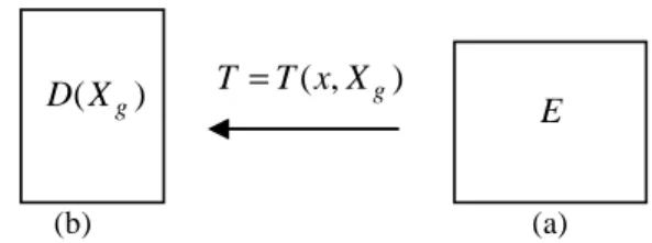
The dimensions of the sensor as well as the thickness of the tube are random input parameters. It means that during the sampling process the geometry is modified. Due to the large number of FV model calls, the remeshing of the geometry adds non negligible computational time. Moreover, the remeshing introduced an additional numerical noise due to the modification of the connectivities between nodes. The GT method is based on changing the position of the coordinates of the nodes without changing their connectivity. First of all an initial mesh is proposed and decomposed into different subdomains, if the coordinates are changed according to the random vector X (vector of geometric random parameters g withXg ⊂ X), then the new mesh is obtained by dilation, compression or translation. The main idea of the GT method is to determine the appropriate transformation. Fig. 3 represents an initial domain and a transformed domain knowing that the new coordinates of X . g

The transformation T transforms the initial domain E into a random domain D X( g). For each realization of X, the nodes are repositioned. Fig. 4 gives the different steps to obtain with the two methods (GT and RM) the stochastic approximate model of the impedance by applying the LAR method.

V. NUMERICAL APPLICATION

A sample of M realizations of the input parameters is generated. With the RM method the geometry and the mesh are recalculated for each realization. Therefore, we estimate the POD for different meshes with a different size, denoted

E

(

g

)

D X

T

=

T x X

( ,

g

)

(b) (a)

Fig. 3 Geometric domain; a) initial domain ( E ); b) transformed domain (D X( g)). k X

GT(Xk) RM(Xk) FV

FV

GT Z

RM Z

LAR

ˆ Z

Fig. 4 Impedance calculation approximation with LAR in both methods: RM and GT.

PODRM. The meshes used have S1=9102, S2= 14504, S3=

19836, S4= 25252 elements.

The second method used is the GT method, in which the mesh is fixed at the beginning (initial mesh) and the appropriate transformation is determined. Meshes of different size are also considered as in RM method (S1, S2, S3, and S4). The process of estimating the POD for the GT method denoted PODGT. For each realization, the GT is used in order

to relocate the nodes according to the modification of the geometry.

In the both methods (RM and GT), the PODRM and PODGT

will be determined with defect sizes a1, a2, and a3 equal to

0.05, 0.4970, and 0.9675mm respectively.

To estimate the POD with two methods, the approximate model is used. It is constructed with N=150 realisations of the FV model obtained with GT or RM method, once the metamodel is constructed, the MCSM is applied with a sample of M =10000 realisations for each value of defect size ai.

Repeating the same process with the RM and GT methods and all meshes. A linear metamodel is constructed and considered in this study; hence, the chaos coefficients are perfectly calculated.

To verify the accuracy of the approximate model, an error is calculated by the following expression:

( ) ( )

1 1 M _ˆ j j j Z X Z X M ε =     = _ − _ 

∑

 (10) The convergence of the metamodel is accurate with an error less than 10-4 which shows that the approximation is of good quality.

TheFig. 5 represents the POD for the S2 mesh, the PODRef

is the reference POD of the GT method with M =10000 and

[

]

Ref 0.06, 0.38, 0.95

POD = ; it shows great agreement with

the two methods (RM and GT) based on LAR and the reference.

The Table I represents the POD for different methods (RM and GT) and for different size meshes (Si) where we can see

also a good agreement between the different methods with changing of the defect size ai. We can see that accurate results

can be obtained with a coarse mesh and we can see also that the RM and GT methods give very similar results for this case meaning that the numerical has really few influence in the considered example.

TABLEI POD FOR DIFFERENT METHODS order PODRM PODGT

a1 a2 a3 a1 a2 a3 S1 P=1 0.06 0.38 0.96 0.06 0.37 0.95 S2 P=1 0.06 0.38 0.95 0.06 0.37 0.95 S3 P=1 0.06 0.39 0.96 0.06 0.35 0.94 S4 P=1 0.06 0.39 0.96 0.06 0.38 0.95 VI. CONCLUSION

In this paper two approaches to estimate the POD of an eddy current testing problem of tube coil system (steam generator tubes) have been estimated. The modification of the geometry which is random has been handled by a geometric

transformation. The geometric transformation (or mapping) is shown to give similar results to the remeshing technic but is less time consuming. The stochastic metamodel has been used in both methods to reduce the computation cost of the high number of realisation and showed a great precision.

REFERENCES

[1] Y. Deng, X. Liu, G. Yang, “Model based POD techniques for enhancing reliability of steam generator tube inspection”, Prognostics and Health

Management (PHM), IEEE Conference, June 2011 , pp. 1-7.

[2] L. Le Gratiet, B. Iooss, G. Blatman, T. Browne, S. Cordeiro and B. Goursaud, “Model assisted probability of detection curves: New statistical tools and progressive methodology”, Journal of Nondestructive Evaluation, 2017, pp. 36-8.

[3] S.Clénet, ”Uncertainty Quantification In Computational Electromagnetics”, The Stochastic Approach, Int. Compumag Soc.

Newslett., Vol. 20,No. 1, March 2013, pp. 2–12.

[4] D. H. Mac, Résolution numérique en électromagnétisme statique de problèmes aux incertitudes géométriques par la méthode de transformation: Application aux machines électriques, Ph.D. dissertation, L2EPLab., ENSAM, Lille, France, 2012.

[5] D. H. Mac, S. Clénet, J.C. Mipo, O. Moreau, “Solution of Static Field Problems With Random Domains”, IEEE Trans. Magn., vol. 46, n°8, p.3385-3388 – 2010.

[6] T. T. Nguyen, S. Clénet, “Influence of Material and Geometric Parameters on the Sensor Based on Active Materials”, IEEE Trans.

Magn., vol. 54, N°. 3, March 2018. pp. 1-4.

[7] T. T. Nguyen, D. H. Mac, S. Clénet, “Uncertainty Quantification Using Sparse Approximation for Models With a High Number of Parameters, Application to a Magnetoelectric Sensor”, IEEE Trans. on Magn., vol. 52, N°. 3, March 2016. pp. 1-4.

[8] S. J. Song, Y. K. Shing, “Eddy current flaw characterization in tubes by neural networks and finite element modelling”, NDT&E international 33, 2000, pp. 233-243.

[9] H.K. Versteeg, W. Malalasekera, ”An Introduction to Computational Fluid Dynamic”, The Finite Volume Method, Longman, 1995.

[10] Nathan Ida, Joao P.A Bastos, “electromagnetic and calculation of field”, Springer-Verlag New York,INC, 1992.

[11] Update on the Tools for Integrity Assessment Project. EPRI, Palo Alto, CA: 2007. 1014756.

[12] R. G. Ghanem., and P. D. Spanos, Stochastic Finite Elements. A Spectral

Approach. Dover, New York, 1991.

[13] O. P. Lemaître, O. M. Knio, Spectral Methods for Uncertainty

Quantification, Springer 2010.

[14] S. N. Rajesh, L. Udpa and S. S. Udpa, “Numerical Model Based Approach for Estimating Probability of Detection in NDE Applications”,

IEEE Trans. on Magn., vol. 29, N°. 2, March 1993. pp. 1857-1860.

0.05 0.2 0.4970 0.8 0.9675 0 0,1 0,3 0,5 0.7 0,9 1 Crack depth a (mm) P ro b a b ili ty O f De te c ti o n POD Ref POD GT POD RM