Science Arts & Métiers (SAM)
is an open access repository that collects the work of Arts et Métiers Institute of Technology researchers and makes it freely available over the web where possible.
This is an author-deposited version published in: https://sam.ensam.eu
Handle ID: .http://hdl.handle.net/10985/8594
To cite this version :
Virginie DARU, Diana BALTEAN-CARLÈS, Catherine WEISMAN, Philippe DEBESSE, Gurunath GANDIKOTA - Two-dimensional numerical simulations of nonlinear acoustic streaming in standing waves - Wave Motion - Vol. 50, p.955-963 - 2013
Two-dimensional numerical simulations of nonlinear
acoustic streaming in standing waves
Virginie Darua,b, Diana Baltean-Carl`esa,c, Catherine Weismana,c, Philippe Debessea, Gurunath Gandikota V. S.a
aLIMSI-UPR CNRS 3251, BP133, 91403 Orsay Cedex
bArts et M´etiers ParisTech, Lab. DynFluid, 151 bd de l’hˆopital, 75013 Paris
cUniversit´e Pierre et Marie Curie, 4 Place Jussieu, 75252 Paris Cedex 05
Abstract
Numerical simulations of compressible Navier-Stokes equations in closed two-dimensional channels are performed. A plane standing wave is excited inside the channel and the associated acoustic streaming is investigated for high intensity waves, in the nonlinear streaming regime. Significant distortion of streaming cells is observed, with the centers of streaming cells pushed towards the end-walls. The mean temperature evolution associated to the streaming motion is also investigated.
Keywords: acoustic streaming, standing wave, numerical simulation, nonlinear streaming regime
1. Introduction
1
Acoustic streaming is generated inside a two-dimensional channel as a
2
consequence of the interaction between a plane standing wave and the solid
3
boundaries. It consists of a mean second order flow produced mainly by shear
4
forces within the viscous boundary layer along the solid walls. This motion
5
was initially studied by Rayleigh [1] in the case of wide channels, in which the
6
boundary layer thickness is negligible in comparison with the channel width.
7
This streaming flow is characterized by four steady counter-rotating vortices
8
outside the boundary layer, nowadays referred to as Rayleigh streaming. The
9
vortices develop along the half wavelength of the standing wave. Along the
10
central axis of the channel, the streaming motion is oriented from acoustic
11
velocity nodes to antinodes. Inside the boundary layer four additional
vor-12
tices are created simultaneously, with the streaming motion oriented from
13
acoustic velocity antinodes to nodes along the inner walls of the tube [2, 3].
14
In the case of wide channels, Menguy and Gilbert [4] showed that
stream-15
ing itself can be linear (case of slow streaming) or nonlinear (case of fast
16
streaming), and both regimes are characterized by a reference nonlinear
17
Reynolds number ReN L = (M × y0/δν)2 reflecting the influence of inertial
18
effects on the streaming flow (M is the acoustic Mach number, M = Umax/c0,
19
with Umax the maximum acoustic velocity inside the channel and c0 the
ini-20
tial speed of sound, y0 is the half width of the channel and δν the viscous
21
boundary layer thickness). Most analytical streaming models have been
es-22
tablished in the case of slow streaming, characterized by ReN L ≪ 1. They
23
are based on successive approximations of the nonlinear hydrodynamic
equa-24
tions and have been derived for arbitrary values of the ratio y0/δν, taking
25
into account the variations of heat conduction and viscosity with
tempera-26
ture [5], and the existence of a longitudinal temperature gradient [6]. In the
27
case ReN L= O(1), Menguy and Gilbert [4] derived an asymptotic model for
28
streaming flow inside wide cylindrical resonators, with no mean temperature
gradient, and showed a distortion of streaming patterns due to inertia
ef-30
fects. However, this model does not cover the strongly nonlinear streaming
31
regime (ReN L ≫ 1), and does not explain the nonlinear effects on acoustic
32
streaming recently observed in several experimental works [7, 8, 9], where
33
the temperature gradient along the resonator wall has a significant influence.
34
Numerical simulations in the linear regime, yielding results for non
ide-35
alized geometries, were performed in the specific cases of thermoacoustic
36
refrigerators [10] or in annular resonators [11] and solved the dynamics of
37
the flow without taking heat transfer into account.
38
Simulations in the nonlinear regime were first performed by Yano [12],
39
who studied the acoustic streaming associated with resonant oscillations with
40
periodic shock waves in tubes with aspect ratio (width over length) very
41
large (0.1). He solved the full 2D Navier-Stokes equations with an upwind
42
finite-difference TVD scheme and showed the existence of irregular vortex
43
structures and even turbulent streaming for high streaming Reynolds
num-44
bers (based on a characteristic streaming velocity, the tube length, and the
45
kinematic viscosity, Rs= UsL/ν). This is a different configuration than our
46
configuration, since it considers low frequency acoustic waves in wide tubes
47
with respect to their length and focuses on turbulent streaming.
48
Simulations of acoustic streaming in the linear and nonlinear regime,
tak-49
ing heat transfer into account, in a two-dimensional rectangular enclosure,
50
were performed by Aktas and Farouk [13]. In their study, the wave is created
51
by vibrating the left wall of the enclosure and the full compressible
Navier-52
Stokes equations are solved, with an explicit time-marching algorithm (a
53
fourth order flux-corrected transport algorithm) to track the acoustic waves.
Their numerical results are in agreement with theoretical results in the
lin-55
ear regime and show irregular streaming motion in the nonlinear regime,
56
but they show the existence of irregular streaming at small values of ReN L,
57
in contradiction with experiments cited above. Moreover, these simulations
58
do not analyze the deformation of the streaming cells until they split onto
59
several cells.
60
We propose in this work to conduct numerical 2D compressible
simula-61
tions for studying the origin of the distortion of streaming cells (of Rayleigh
62
type) that were experimentally observed. Calculations are performed for
63
channels with aspect ratios ranging from 0.01 to 0.07, and the coupling
be-64
tween streaming effects and thermal effects in the channel (existence of a
65
mean temperature gradient) is also investigated.
66
2. Problem description and numerical model
67
We consider a rectangular channel of length L and half width y0, initially
68
filled with the working gas. In order to initiate an acoustic standing wave in
69
the channel, it is shaken in the longitudinal direction (x), so that an harmonic
70
velocity law is imposed, V(t) = (V (t), 0)T, with V (t) = xpω cos(ωt), ω being
71
the angular frequency and xp the amplitude of the channel displacement.
72
The channel being undeformable, the flow can be modeled by the
compress-73
ible Navier-Stokes equations expressed in the moving frame attached to the
channel, so that a forcing source term is added. The model reads: 75 ∂ρ ∂t +∇ · (ρv) = 0 ∂ρv ∂t +∇ · (ρv ⊗ v) + ∇p = ∇ · (¯¯τ) − ρ dV dt ∂ρE ∂t +∇ · (ρEv + pv) = ∇ · (k∇T ) + ∇ · (¯¯τv) − ρv · dV dt (1)
where v = (u, v)T is the flow velocity, E = e + 1
2v· v is the total energy,
76
with e = (γ−1)ρp the internal energy, γ the specific heat ratio, ¯τ =¯ −23µ(∇ ·
77
v)¯¯I + 2µ ¯¯D the viscous stress tensor of a Newtonian fluid, ¯¯D the strain tensor,
78
µ the dynamic viscosity, k the thermal conductivity. The thermo-physical
79
properties µ and k are supposed to be constant. The gas is considered as
80
a perfect gas obeying the state law p = rρT , where T is the temperature
81
and r is the perfect gas constant corresponding to the working gas. The
82
physical boundary conditions employed in the moving frame are: no slip and
83
isothermal walls.
84
The model is numerically solved by using high order finite difference
85
schemes, developed in Daru and Tenaud [14]. An upwind scheme, third
86
order accurate in time and space, is used for convective terms, and a
cen-87
tered scheme, second order, is used for diffusion terms. More detail about
88
the scheme and computations showing its good qualities can be found in
89
Daru and Gloerfelt [15], Daru and Tenaud [16]. This scheme can be derived
90
up to an arbitrary order of accuracy for convective terms in the case of a
91
scalar equation. Here the third order scheme is selected, after having done
92
several comparisons using higher order schemes (up to the 11th order), that
93
have shown that third order gives sufficient accuracy for a reasonable CPU
94
cost. In cases where shock waves are present, the scheme can be equipped
with a flux limiter (MP), preserving monotonicity, intended for suppressing
96
the parasitic numerical oscillations generated in the shock region, while
pre-97
serving the accuracy of the scheme in smooth regions. However, the flows
98
considered here are always low Mach number flows. Although traveling shock
99
waves are a main feature of the flow for high acoustics levels, as noticed by
100
several authors [17], they are of weak intensity and the numerical oscillations
101
are very small and do not spoil the solution. Thus the MP limiter, which
102
is expensive in terms of CPU cost, was not activated in these calculations.
103
For solving the 2D Navier-Stokes equations, the scheme is implemented using
104
Strang splitting. This reduces the formal accuracy of the scheme to second
105
order. However, numerical experiments have shown that a very low level of
106
error is still achieved.
107
Let us describe our numerical procedure. The system (1) can be written
108 in vector form : 109 ∂w ∂t + ∂ ∂x(f − f v) + ∂ ∂y(g− g v) = h (2)
where w is the vector of conservative variables (ρ, ρu, ρv, ρE)T, f and g are
110
the inviscid fluxes f = (ρu, ρu2+ p, ρuv, ρEu + pu)T and g = (ρv, ρuv, ρv2+
111
p, ρEv + pv)T, fv and gv being the viscous fluxes fv = (0, τxx, τxy, k∂T∂x +
112
uτxx+ vτxy)T, gv = (0, τxy, τyy, k∂T∂y + uτxy + vτyy)T. The source term reads
113
h = (0,−ρdVdt, 0,−ρudVdt)T. Denoting wni,j the numerical solution at time t =
114
nδt and grid point (x, y) = (iδx, jδy), we use the following Strang splitting
115
procedure to obtain second order of accuracy every two time steps :
116
wi,jn+2 = LδxLδyLδyLδxwnij (3) where Lδx (resp. Lδy) is a discrete approximation of Lx(w) = w + δt(−fx+
fv
x + h) (resp. Ly(w) = w + δt(−gy + gvy)). The 1D operators being similar
118
in the two directions, we only describe the x operator. The scheme is
imple-119
mented as a correction to the second order MacCormack scheme. It consists
120
of three steps, as follows :
121
wi,j∗ = wni,j− δxδt(fi+1,j − fi,j − fi+1/2,jv + fiv−1/2,j)n+ δt hni,j wi,j∗∗ = w∗i,j− δxδt(fi,j − fi−1,j− fi+1/2,jv + fiv−1/2,j)∗
wi,jn+1 = 12(wi,jn + w∗∗i,j) + Ci+1/2,jx − Cix−1/2,j
(4)
The viscous fluxes are discretized at each interface using centered second
or-122
der finite differences formulae. The corrective term Ci+1/2,jx −Cix−1/2,j provides
123
the third order accuracy and the upwinding for the inviscid terms. Let us
de-124 fine ψi+1/2,j = 16 ∑4 l=1 { |νl i+1/2,j|(1 − ν l i+1/2,j)(1 + ν l i+1/2,j)δα l i+1/2,j · d l i+1/2,j } , 125 where νl = δt δxλ
l, λl and dl are the eigenvalues and eigenvectors of the
Roe-126
averaged jacobian matrix A = dwdf [18], and δαl is the contribution of the
127
l−wave to the variation (wn
i+1/2,j− w n
i−1/2,j). Using the function ψ, the
cor-128
rective term reads :
129 Ci+1/2,jx = −ψn i+1/2,j+ ψ n i−1/2,j if νi+1/2,j ≥ 0 ψi+3/2,jn − ψni+1/2,j if νi+1/2,j < 0
(5)
This completes the description of the numerical method.
130
We are interested in the acoustic streaming generated by the interaction of
131
the imposed plane standing wave and the channel wall. Resonant conditions
132
are imposed, for which L = λ/2, λ = c0/f being the wave length, c0 the speed
133
of sound for initial state and f the vibration frequency of the channel. It is
134
known [5] that boundary layers develop along the walls, with thickness δν =
135
√
2ν/ω, ν being the kinematic viscosity ν = µ/ρ0, and ρ0the density at initial
136
state. Depending on the value of the ratio y0/δν, several patterns of streaming
can appear: Rayleigh-type streaming in the central region, and boundary
138
layer type streaming near the longitudinal walls. The boundary layer is of
139
small thickness and must be correctly resolved by the discretization mesh.
140
After several trials, we have determined that a value of 5 points per boundary
141
layer thickness is sufficient for reasonable accuracy of the simulations. The
142
results obtained using 10 points per boundary layer thickness show very small
143
differences with the former, the maximum value of the differences being less
144
than 3%. All results presented below are thus obtained using a cartesian
145
mesh of rectangular cells of constant size δx and δy, composed of 500 points
146
in the axial direction x, and of 5× y0/δν points in the y direction normal to
147
the axis. In the considered geometry, this leads to cells such that δy ≪ δx.
148
The flow being symmetrical with respect to the x axis (at least in the range
149
of parameters treated), only the upper half of the channel was considered.
150
Also, the scheme being fully explicit, the time step δt is fixed such as to
151
satisfy the stability condition of the scheme which can be written as:
152
δt≤ 1
2min(δy
2
/ν, δy2/(k/ρ0c0), δy/c0) (6)
As shown in Equation (6), the first two limiting values δy2/ν and δy2/(k/ρ 0c0)
153
are related to the viscous and thermal conduction terms, and the third one
154
δy/c0 is related to the acoustic propagation. In all cases considered here,
155
the time step limitation is acoustic, ie δt≤ 1
2δy/c0. Taking δt = 1
2δy/c0 and
156
δy = δν/5, this results in a number of time steps NT per period of oscillation
157 proportional to √L, NT = 1/(f δt) = 10 √ 2πc0 ν √
L. Since transients of
sev-158
eral hundreds of periods may be needed in order to reach stabilized steady
159
streaming flow, simulations are very costly, and one must rely on numerical
160
schemes that are sufficiently accurate in both space and time.
Finally, the mean flow is obtained from calculating a simple mean value
162
for each physical quantity (velocity, pressure, temperature) over an acoustic
163
period. The mean velocity obtained is the so-called Eulerian streaming
ve-164
locity. The Lagrangian streaming velocity, associated to the streaming mass
165
transport, could also be computed. The difference between them is
signifi-166
cant only in the boundary layer, and in the case of wide channels the two
167
velocities are almost the same. In order to observe the mechanism of cell
168
distortion, either one of these velocities can be monitored.
169
3. Numerical results
170
We consider a channel initially filled with air at standard
thermody-171
namic conditions, p0 = 101325Pa, ρ0 = 1.2kgm−3, T0 = 294.15K. The
172
thermo-physical properties of air are µ = 1.795 10−5kgm−1s−1 and k =
173
0.025Wm−1K−1. Also for air, γ = 1.4 and r = 287.06Jkg−1K−1. The
174
Prandtl number P r is equal to 0.726. This results in an initial speed of
175
sound c0 = 343.82ms−1.
176
For a 1m long channel, the limiting time step would correspond to NT ≈
177
25000√L, that is 25000 iterations per period. Since transients of several
178
hundreds of periods may be needed in order to reach stabilized streaming
179
flow, several millions of iterations are necessary for each simulation.
Con-180
sidering these numerical constraints, a shorter channel is considered, with
181
L = 8.59mm. This corresponds to a high-frequency wave, with f = 20000Hz.
182
The resulting boundary layer thickness is δν = 1.54 10−5m. The time step
183
δt = 8 10−9s is chosen in order to satisfy the numerical stability condition,
184
corresponding to 6250 time iterations per period for a mesh involving 5 grid
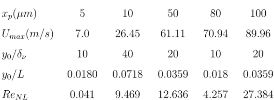
xp(µm) 5 10 50 80 100 Umax(m/s) 7.0 26.45 61.11 70.94 89.96
y0/δν 10 40 20 10 20
y0/L 0.0180 0.0718 0.0359 0.018 0.0359
ReN L 0.041 9.469 12.636 4.257 27.384
Table 1: Values of the parameters of the simulations.
points across the boundary layer thickness. The acoustic velocity produced
186
in the channel depends on the amplitude of the channel displacement and on
187
the ratio y0/δν. It varies approximately linearly with the amplitude of the
188
channel displacement, for a given ratio y0/δν. Table 1 summarizes the
dif-189
ferent parameter values corresponding to the simulations that are presented
190
thereafter.
191
As mentioned earlier, the parameter identified as relevant in describing
192
the regularity of streaming flow is the nonlinear Reynolds number ReN L
193
introduced by Menguy and Gilbert [4]. In this paper we used a slightly
194
different definition for ReN L, because the definition of the viscous boundary
195
layer thickness is different. Our Reynolds number corresponds to half of that
196
of Menguy and Gilbert [4].
197
We first present results concerning the main acoustic field in the channel,
198
for a small value of ReN L corresponding to slow streaming. In Figure 1(a)
199
is represented the velocity signal at the center of the channel, as a function
200
of the number of periods elapsed. At this location, the acoustic velocity
201
amplitude is maximum since it corresponds to the antinode. For this value
202
of ReN L, the problem is nearly linear and the final signal is purely
soidal, in agreement with the linear theory. The amplification of the initial
204
perturbation until saturation can be observed. The periodic regime is
estab-205
lished after about 20 periods. Figure 1(b) shows the time evolution of the
206
mean horizontal velocity (over an acoustic period) and of the mean
temper-207
ature difference ∆T = T − T0 (also over an acoustic period) on the axis,
208
at x = λ/8. At this location the streaming velocity is maximum. It can be
209
noticed that the steady streaming field is established also after about 20
peri-210
ods which is of the same order of magnitude as the theoretical characteristic
211
streaming time scale τc = (2yπ0)2 1ν, (see Amari, Gusev and Joly [19]) which
212
in this case gives nc periods for reaching steady-state, with nc= 13. In
Fig-213
ure 2(a) is shown the variation of the axial dimensionless streaming velocity
214
at x = λ/8 along the channel’s width, compared with results computed
us-215
ing the analytical expressions of Hamilton, Ilinskii and Zabolotskaya [20]. In
216
this figure, the reference velocity is the Rayleigh streaming reference velocity
217
[2, 5], uRayleigh = 163 Umax2 /c0. The slight discrepancy between the numerical
218
and the analytical profiles is probably due to the presence of the vertical
219
end walls, which is not accounted for in the model of Hamilton, Ilinskii and
220
Zabolotskaya [20]. In Figure 2(b) is shown the stabilized mean pressure p−p0
221
(over an acoustic period), scaled by (γ/4)p0M2, along the channel’s axis. It
222
is the second order average pressure resulting from the streaming flow, which
223
is clearly one-dimensional and has a cosine variation with respect to x, as
224
expected in the linear regime of streaming. In the present case, there is an
225
offset pressure poff, corresponding to an increase of the mean pressure and
226
temperature (uniform in space) inside the channel, due to the harmonic
forc-227
ing source term. When subtracting off this offset pressure, the theoretical
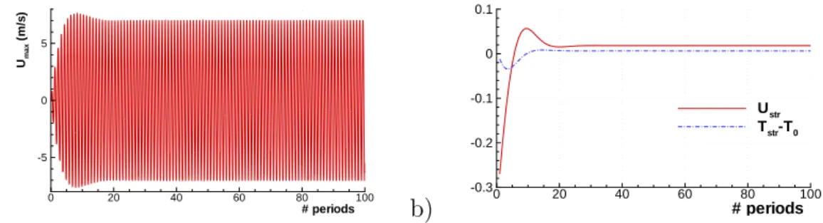
a) # periods Um a x (m /s ) 0 20 40 60 80 100 -5 0 5 b) # periods 0 20 40 60 80 100 -0.3 -0.2 -0.1 0 0.1 Ustr Tstr-T0
Figure 1: a) Acoustic velocity at the channel’s center, as a function of time counted by the number of periods elapsed. b) Mean horizontal velocity and mean temperature variation, on the channel’s axis at x = λ/8. Case ReN L= 0.041 (y0/δν = 10, M = 0.02).
a) Ust y /y0 -1 -0.5 0 0.5 1 0 0.2 0.4 0.6 0.8 1 ReNL=0.041 Hamilton x=λ/8 b) x/L pst 0 0.2 0.4 0.6 0.8 1 -1.5 -1 -0.5 0 0.5 1 1.5
Figure 2: a) Ustas a function of y/y0at x = λ/8, numerical (present study) and analytical
[20] results. b) Dimensionless mean fluctuating pressure, p− p0 along the channel’s axis.
Case ReN L= 0.041 (y0/δν = 10, M = 0.02).
result for the dimensionless hydrodynamic streaming pressure is obtained,
229
P2s = cos 4πxλ (see Menguy and Gilbert [4]).
230
Simulations are then performed for several values of ReN L
correspond-231
ing to configurations ranging from slow streaming flow (ReN L = 0.041) to
232
fast streaming flow (ReN L = 27.384), for several values of the cavity width
233
(y0/δν = 10, 20, 40), and for increasing acoustic velocities, with Mach
num-234
bers ranging from M = 0.02 to M = 0.27 so that shock waves can occur.
235
This can be seen in Figure 3(right) showing the acoustic velocity signal at
236
channel’s center as a function of time counted by the number of periods
elapsed. In Figure 3(a)(right) the signal contains only one frequency, but for
238
all other cases, there are shock waves and the acoustic velocity signal is
dis-239
torted in a ”U” shape, because of the presence of odd harmonics (3, 5, etc).
240
Figure 3(left) shows the streamlines of the streaming velocity field over the
241
whole length and only over the top half width of the channel. As expected, in
242
the case of small ReN L number values (Figure 3(a)), four symmetric
stream-243
ing cells develop over the length and the half width of the channel: two cells
244
in the boundary layer, and two cells in the core of the channel, identified in
245
the literature as Rayleigh streaming. These results are in agreement with
246
the predictions of analytical models of streaming flows [5, 6], and with
ex-247
perimental measurements [7]. The only noticeable difference is the slight
248
asymmetry of cells with respect to the vertical lines x = λ/8 and x = 3λ/8,
249
due to the presence of vertical boundary layers. Indeed these boundary layers
250
are accounted for in the present simulations but are neglected in the
analyt-251
ical models, and are very far from the measurement area in the experiments.
252
Several simulations have shown that this asymmetry is independent of ReN L
253
as long as the value of the latter remains small with respect to 1.
254
For ReN L > 1, the steady streaming flow is established after the same
255
characteristic time as in the linear case. The recirculation cells become very
256
asymmetric as ReN L increases, and streaming flow becomes irregular
(Fig-257
ure 3(b,c,d,e)(left)). This was also observed experimentally (with PIV
mea-258
surements) by Nabavi, Siddiqui and Dargahi [8] in a rectangular enclosure.
259
The centers of all streaming cells (boundary layer cells as well as central
260
cells) are displaced towards the ends of the resonant channel, close to the
261
boundary layers next to the vertical walls. PIV measurements by Nabavi,
Siddiqui and Dargahi [8] show the same distortion of streamlines between an
263
acoustic velocity node and an antinode. Figure 4(a) shows the x variation
264
along the channel’s central axis y = 0, of the axial dimensionless streaming
265
velocity component, using as reference velocity the Rayleigh streaming
ref-266
erence velocity [2, 5], uRayleigh = 163Umax2 /c0. There is a clear modification of
267
the velocity profiles as ReN L increases: the sine function associated to slow
268
streaming becomes steeper next to the channel’s ends. The slope to the curve
269
at the channel’s center (acoustic velocity node) becomes smaller as ReN L
in-270
creases, then becomes close to zero (curve parallel to the longitudinal axis) for
271
a critical value between 13 and 27, and then changes sign, which indicates the
272
emergence of new streaming cells (Figure 4(a)). Another consequence of the
273
distortion of streaming cells can be observed on the acoustic streaming axial
274
velocity profiles along the width of the channel, shown in Figure 4(b,c,d).
275
The parabolic behavior in the center of the channel at x = λ/8 disappears
276
as ReN L increases (see Figure 4(b)), as a consequence of displacement of the
277
center of each streaming cell toward the velocity node. Figures 4(c,d) also
278
confirm the direction of the displacement of the streaming cells’ centers. This
279
distortion of streaming cells was already observed in experiments in
rectan-280
gular or cylindrical geometries in wide channels [7, 8, 9]. Nabavi, Siddiqui
281
and Dargahi [8] described it as irregular streaming and detected a critical
282
nonlinear Reynolds number ReN L = 25 that separates regular and
irregu-283
lar streaming, which is in agreement with our simulations. In the literature
284
there is to our knowledge no other theoretical or numerical study confirming
285
measurements in these streaming regimes. With the weakly nonlinear model
286
of Menguy and Gilbert [4] the streaming can be calculated for a maximum
value of ReN L = 2 (in our definition), while the numerical simulations of
288
Aktas and Farouk [13] show the existence of multiple streaming cells for a
289
low value of ReN L = 1.4, which is in contradiction with our results and with
290
experiments. Moreover, these numerical simulations [13] do not analyse in
291
detail the transition from two exterior streaming cells to more streaming
292
cells.
293
According to Menguy and Gilbert [4], the fluid inertia causes distortion
294
of streaming cells for large values of ReN L. This was also verified through our
295
simulations. For ReN L = O(1), the Mach number is still small (the wave is
296
almost a mono-frequency wave) and the mean temperature difference inside
297
the channel is smaller than 0.1K (the mean temperature gradient is
negligi-298
ble). The approximations of the model by Menguy and Gilbert [4] still apply
299
here, so we can say that the distortion is caused only by inertial effects. When
300
ReN L increases, periodic shocks appear and the mean temperature gradient
301
becomes important in our simulations. In their experimental study,
Thomp-302
son, Atchley and Maccarone [9] show the existence of some distortion of the
303
streaming field that are not predicted by existing models of the literature in
304
the nonlinear regime. They do not relate this distortion to fluid inertia but
305
rather to the influence of the mean temperature field, and more specifically
306
of the axial temperature gradient induced through a thermoacoustic effect
307
along the horizontal walls of the resonating channel. In an experimental case
308
with no shock waves, Merkli and Thomann [17] showed that a mean
tem-309
perature gradient is established inside the tube so that heat is removed close
310
to the velocity antinodes, i.e. at the location of largest viscous dissipation,
311
and heat is produced close to velocity nodes, along the lateral walls. Similar
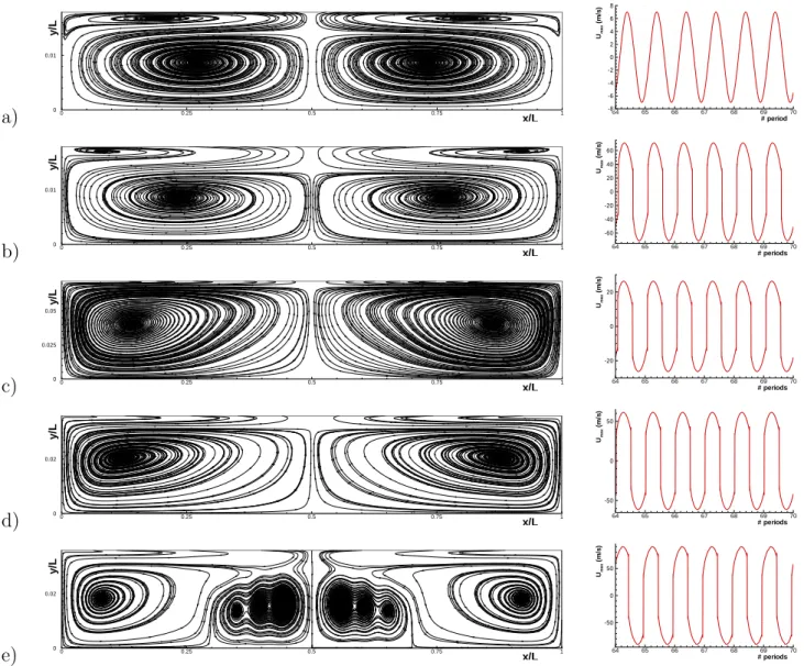
a) x/L y /L 0 0.25 0.5 0.75 1 0 0.01 # period Um a x (m /s ) 64 65 66 67 68 69 70 -8 -6 -4 -2 0 2 4 6 8 b) x/L y /L 0 0.25 0.5 0.75 1 0 0.01 # periods Um a x (m /s ) 64 65 66 67 68 69 70 -60 -40 -20 0 20 40 60 c) x/L y /L 0 0.25 0.5 0.75 1 0 0.025 0.05 # periods Um a x (m /s ) 64 65 66 67 68 69 70 -20 0 20 d) x/L y /L 0 0.25 0.5 0.75 1 0 0.02 # periods Um a x (m /s ) 64 65 66 67 68 69 70 -50 0 50 e) x/L y /L 0 0.25 0.5 0.75 1 0 0.02 # periods Um a x (m /s ) 64 65 66 67 68 69 70 -50 0 50
Figure 3: Streamlines of mean flow on the top half of the channel (left) and acoustic velocity signal at channel’s center as a function of time counted by the number of periods elapsed (right) a) ReN L= 0.041 (y0/δν = 10, M = 0.02). b) ReN L= 4.257 (y0/δν = 10,
M = 0.206). c) ReN L= 9.469 (y0/δν = 40, M = 0.077). d) ReN L= 12.636 (y0/δν = 20,
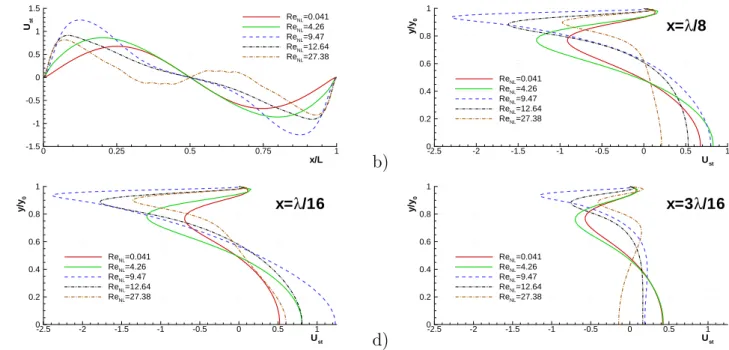
a) x/L Us t 0 0.25 0.5 0.75 1 -1.5 -1 -0.5 0 0.5 1 1.5 ReNL=0.041 ReNL=4.26 ReNL=9.47 ReNL=12.64 ReNL=27.38 b) Ust y /y0 -2.5 -2 -1.5 -1 -0.5 0 0.5 1 0 0.2 0.4 0.6 0.8 1 ReNL=0.041 ReNL=4.26 ReNL=9.47 ReNL=12.64 ReNL=27.38 x=λ/8 c) Ust y /y0 -2.5 -2 -1.5 -1 -0.5 0 0.5 1 0 0.2 0.4 0.6 0.8 1 ReNL=0.041 ReNL=4.26 ReNL=9.47 ReNL=12.64 ReNL=27.38 x=λ/16 d) Ust y /y0 -2.5 -2 -1.5 -1 -0.5 0 0.5 1 0 0.2 0.4 0.6 0.8 1 ReNL=0.041 ReNL=4.26 ReNL=9.47 ReNL=12.64 ReNL=27.38 x=3λ/16
Figure 4: Horizontal mean velocity component Ust, normalized with 163U 2
max/c0 for the 5
cases of Figure 3. a) Ust along the channel’s central axis. b),c) and d) Ust as a function
a) x/L y /L 0 0.25 0.5 0.75 1 0 0.01 294.13 294.138 294.146 294.154 294.162 b) x/L y /L 0 0.25 0.5 0.75 1 0 0.01 291.8 292.6 293.4 294.2 295 295.8 296.6 297.4 c) x/L y /L 0 0.25 0.5 0.75 1 0 0.02 292 294 296 298 300 302 304 306 308 310 d) x/L y /L 0 0.25 0.5 0.75 1 0 0.02 292 296 300 304 308 312 316 320 324 328 332
Figure 5: Mean temperature field on the top half of the channel, a) ReN L = 0.041. b)
ReN L= 4.257. c) ReN L= 12.636. d) ReN L= 27.383. The difference between minimum
and maximum values of temperature is (respectively) : a) ∆T = 0.039K, b) ∆T = 6.39K, c) ∆T = 19.4K, d) ∆T = 44K.
observations can be made in our simulations as seen in Figure 5(a) which
313
shows the mean temperature field for small values of ReN L. The
thermoa-314
coustic heat transport takes place at a distance of one thermal boundary
315
layer thickness and then heat diffuses in the radial direction, yielding a
tem-316
perature field almost one-dimensional in the central part of the tube in the
317
steady-state. As ReN Lincreases however, the mean temperature field clearly
318
becomes two-dimensional, as a consequence of both convective heat
trans-319
port by streaming flow and heat conduction in both directions (Figure 5(b)).
320
Within the considered range of values of the nonlinear Reynolds number,
321
there is a change of regime for the temperature field before ReN L = 13.26,
322
corresponding to the confinement of outer streaming cell towards the
acous-323
tic velocity node. Consequently a zone of very small streaming velocities is
324
generated in the middle of the cavity and that induces the accumulation of
325
heat (Figure 5(c)). The mean temperature gradient changes the orientation
326
and can cause the splitting of the outer cell into several cells when further
327
increasing ReN L (Figure 5(d)).
328
Note that the streaming flow stabilizes in several stages in regimes with
329
high values of the nonlinear Reynolds number. In a first and rapid stage
330
(a few tens of periods), regular streaming flow appears. Then this regular
331
streaming is destabilized along with increasing heterogeneity of the mean
332
temperature field. The steady mean flow stabilizes much later, with time
333
scales related to convection and heat conduction.
4. Conclusions
335
The numerical simulations performed demonstrate the transition from
336
regular acoustic streaming flow towards irregular streaming, in agreement
337
with existing experimental data. These are the first simulations, to our
338
knowledge, in good alinement with experiments of nonlinear streaming regimes.
339
Results show a sizable influence of vertical boundary layers for the chosen
340
configuration. There is also intricate coupling between the mean
tempera-341
ture field and the streaming flow. This coupling effect will be the object of
342
future work. Also, extension of current results in configurations with larger
343
channels is currently in progress.
344
Acknowledgements
345
The authors wish to acknowledge many fruitful discussions with Jo¨el
346
Gilbert and H´el`ene Bailliet.
347
References
348
[1] Lord Rayleigh, On the circulation of air observed in Kundts tubes, and
349
on some allied acoustical problems, Philos. Trans. R. Soc. London 175
350
(1884) 1-21.
351
[2] W.L. Nyborg, Acoustic streaming, in Physical Acoustics, W. P. Mason
352
(ed), Academic Press, New York Vol. 2B (1965) 265-331.
353
[3] H. Schlichting, Berechnung ebener periodischer Grenzschicht-
strom-354
mungen [calculation of plane periodic boundary layer streaming], Phys.
355
Zcit. 33 (1932) 327-335.
[4] L. Menguy, J. Gilbert, Non-linear Acoustic Streaming Accompanying a
357
Plane Stationary Wave in a Guide, Acta Acustica 86 (2000) 249-259.
358
[5] M.F. Hamilton, Y.A. Ilinskii, E.A. Zabolotskaya, Acoustic streaming
359
generated by standing waves in two-dimensional channels of arbitrary
360
width, J. Acoust. Soc. Am. 113(1) (2003) 153-160.
361
[6] H. Bailliet, V. Gusev, R. Raspet, R.A. Hiller, Acoustic streaming in
362
closed thermoacoustic devices, J. Acoust. Soc. Am. 110 (2001)
1808-363
1821.
364
[7] S. Moreau, H. Bailliet, J.-C. Vali`ere, Measurements of inner and outer
365
streaming vortices in a standing waveguide using laser doppler
velocime-366
try, J. Acoust. Soc. Am. 123(2) (2008) 640-647.
367
[8] M. Nabavi, K. Siddiqui, J. Dargahi, Analysis of regular and irregular
368
acoustic streaming patterns in a rectangular enclosure, Wave Motion 46
369
(2009) 312-322.
370
[9] M.W. Thompson, A.A. Atchley, M.J. Maccarone, Influences of a
tem-371
perature gradient and fluid inertia on acoustic streaming in a standing
372
wave, J. Acoust. Soc. Am. 117(4) (2004) 1839-1849.
373
[10] D. Marx, P. Blanc-Benon, Computation of the mean velocity field above
374
a stack plate in a thermoacoustic refrigerator, C.R. Mecanique 332
375
(2004) 867-874.
376
[11] A. Boufermel, N. Joly, P. Lotton, M. Amari, V. Gusev, Velocity of
377
Mass Transport to Model Acoustic Streaming: Numerical Application
378
to Annular Resonators, Acta Acust. United Acust. 97(2) (2011) 219-227.
[12] T. Yano, Turbulent acoustic streaming excited by resonant gas
oscilla-380
tion with periodic shock waves in a closed tube, J. Acoust. Soc. Am.
381
106 (1999) L7-L12.
382
[13] M.K. Aktas, B. Farouk, Numerical simulation of acoustic streaming
383
generated by finite-amplitude resonant oscillations in an enclosure,
384
J. Acoust. Soc. Am. 116(5) (2004) 2822-2831.
385
[14] V. Daru, C. Tenaud, High Order One-step Monotonicity-Preserving
386
Schemes for Unsteady Compressible flow Calculations, Journal of
Com-387
putational Physics 193 (2004) 563- 594.
388
[15] V. Daru, X. Gloerfelt, Aeroacoustic computations using a high order
389
shock-capturing scheme, AIAA Journal 45(10) (2007) 2474-248.
390
[16] V. Daru, C. Tenaud, Numerical simulation of the viscous shock tube
391
problem by using a high resolution monotonicity preserving scheme,
392
Computers and Fluids 38(3) (2009) 664-676.
393
[17] P. Merkli, H. Thomann, Thermoacoustic effects in a resonance tube, J.
394
Fluid Mech. 70(1) (1975) 161-177.
395
[18] P.L. Roe, Approximate Riemann solvers, parameter vectors and
differ-396
ence schemes, Journal of Computational Physics, 43 (1981) 357-372.
397
[19] M. Amari, V. Gusev, N. Joly, Temporal dynamics of the sound wind in
398
acoustitron, Acta Acustica united with Acustica 89 (2003) 1008-1024.
399
[20] M.F. Hamilton, Y.A. Ilinskii, E.A. Zabolotskaya, Thermal effects on
acoustic streaming in standing waves, J. Acoust. Soc. Am. 114(6) (2003)
401
3092-3101.