MATLAB script for slope stability calculations with
COMSOL Multiphysics
by
Salah AHMED
THESIS PRESENTED TO ÉCOLE DE TECHNOLOGIE SUPÉRIEURE
IN PARTIAL FULFILLMENT FOR A MASTER’S DEGREE
WITH THESIS IN CONSTRUCTION ENGINEERING
M.A.Sc.
MONTREAL, AUGUST 8, 2017
ÉCOLE DE TECHNOLOGIE SUPÉRIEURE
UNIVERSITÉ DU QUÉBEC
© Copyright reserved
It is forbidden to reproduce, save or share the content of this document either in whole or in parts. The reader who wishes to print or save this document on any media must first get the permission of the author.
BOARD OF EXAMINERS
THIS THESIS HAS BEEN EVALUATED BY THE FOLLOWING BOARD OF EXAMINERS
Mr. François Duhaime, Thesis Supervisor
Construction Engineering Department at École de technologie supérieure
Mr. Yannic Ethier, Thesis Co-supervisor
Construction Engineering Department at École de technologie supérieure
Mr. Lotfi Guizani, President of the Board of Examiners
Construction Engineering Department at École de technologie supérieure
Mr. Michel Vaillancourt, Member of the jury
Construction Engineering Department at École de technologie supérieure
THIS THESIS WAS DEFENDED
IN THE PRESENCE OF A BOARD OF EXAMINERS AND PUBLIC JULY 26, 2017
ACKNOWLEDGMENT
I would like to thank my supervisor Professor Francois Duhaime for his excellent guidance, patience, availability, and support, and for providing me with an excellent atmosphere during the last two years. I would like to thank him also for encouraging me to increase my knowledge about research in general and programming more specifically. Finally, I would like to thank him for his patience and cooperation during the thesis writing and correction period.
I would like to thank my co-supervisor, Yannic Ethier, for his patience, humility and kindness, especially during the course period. I would like to thank him for his understanding and support during my Master.
I would also like to thank my parents. They always supported and encouraged me with their best wishes. Finally, I would like to thank my wife. She has always supported me through both good and bad times.
MATLAB SCRIPT FOR SLOPE STABILITY CALCULATIONS WITH COMSOL MULTIPHYSICS
Salah AHMED
RÉSUMÉ
Un nouveau script MATLAB a été développé et programmé pour la réalisation d’analyses de stabilité de pente avec le logiciel d’éléments finis (EF) COMSOL Multiphysics. Le script MATLAB calcule un facteur de sécurité basé sur le champ de contraintes calculé avec COMSOL Multiphysics. Les contraintes sont calculées en supposant un comportement linéaire-élastique basé sur un module d’Young et un coefficient de Poisson. Le script permet de tester une série de surfaces de rupture circulaires définies par les coordonnées de leur centre et leur rayon. Le script vérifie tout d’abord l’intersection de la pente et de la surface de rupture. La portion de la surface de rupture à l’intérieur de la pente est ensuite divisée en une série de tranches d’égales largeurs. Les contraintes sont calculées au centre de la base de chaque tranche le long de la surface de rupture. Les tenseurs des contraintes subissent ensuite une rotation en fonction de l’angle de la base de chaque tranche pour calculer les contraintes normales et de cisaillement. Les contraintes normales sont utilisées avec les paramètres de Mohr-Coulomb pour calculer la résistance au cisaillement. La contrainte de cisaillement mobilisée correspond à la contrainte de cisaillement calculée avec la méthode des EF. Finalement, un facteur de sécurité global est calculé en se basant sur le rapport entre la somme des forces de résistance et la somme des forces mobilisées. Le nouveau script a été vérifié avec le code d’éléments finis SIGMA/W pour le calcul des contraintes et avec SLOPE/W pour les calculs de facteurs de sécurité. Quatre pentes différentes ont été utilisées pour la vérification du code : une pente uniforme, une pente en gradins, une pente raide et une pente uniforme dans un dépôt de sol stratifié. Les mêmes surfaces de rupture critiques avec des facteurs de sécurité similaires ont été obtenues avec le script MATLAB et avec SLOPE/W. Le nouveau code MATLAB permet d’étendre la gamme d’applications géotechniques multiphysiques pouvant être étudiées avec COMSOL. La thèse fournit aussi une série de recommandations pour améliorer le script MATLAB. Il est entre autres suggéré de programmer une méthode d’analyse par réduction de force, de vérifier le code avec des exemples impliquant une pression interstitielle et de réaliser l’intégration des forces directement dans COMSOL en utilisant des couplages d’intégration.
Mots-clés: stabilité de la pente, analyse par éléments finis, COMSOL Multiphysics, script
programmation MATLAB, surface de glissement critique, résistance au cisaillement, contrainte de cisaillement mobilisée, facteur de sécurité.
MATLAB SCRIPT FOR SLOPE STABILITY CALCULATIONS WITH COMSOL MULTIPHYSICS
Salah AHMED
ABSTRACT
A new MATLAB script was developed and implemented to conduct slope stability analyses with finite element (FE) software COMSOL Multiphysics. The MATLAB script computes a factor of safety based on the finite element stress field calculated with COMSOL. The stresses are calculated based on a linear-elastic behaviour using a Young’s modulus and a Poisson’s ratio. The script is programmed to test a series of circular slip surfaces defined by their centre coordinates and their radius. The script first verifies the intersection between the slope geometry and slip surface. The intersecting part is then divided into a series of equal-width vertical slices. Stresses are calculated from the COMSOL model at the middle point of the base of each slice along the slip surface. The FE stress tensor is then rotated based on the inclination of the slice base to calculate the normal and shear stresses. The normal stress values are used with Mohr-Coulomb parameters to compute the shear strength. The mobilized shear stress was assumed to be equal to the FE shear stress values. Finally, a global factor of safety is calculated based on the ratio between the sum of resisting forces and the sum of mobilized forces. The new script was verified using FE code SIGMA/W to calculate the stresses and using SLOPE/W for factor of safety calculations. The verification was conducted using four different slopes: a uniform slope, a slope with benches, a steep slope, and a uniform slope in a layered soil deposit. The same critical slip surfaces with similar factor of safety values were obtained with the MATLAB script and with the SLOPE/W analysis. The new MATLAB code extends the realm of potential multiphysics applications in geotechnical engineering that can be studied with COMSOL. The thesis also makes recommendations to further improve the MATLAB script. It is suggested to program a strength reduction method, to verify the code with examples involving a pore water pressure, and to perform the force integration directly in COMSOL using integration couplings.
Keywords: Slope stability, finite element analysis, COMSOL Multiphysics, MATLAB
TABLE OF CONTENTS
Page
INTRODUCTION ...1
CHAPTER 1 LITERATURE REVIEW ...3
1.1 Limit equilibrium methods ...3
1.1.1 Principles of limit equilibrium methods ... 4
1.1.2 Main limit equilibrium methods ... 6
1.1.2.1 Swedish method ... 6
1.1.2.2 Bishop method ... 7
1.1.2.3 Morgenstern and Price method ... 9
1.2 Finite element and finite difference methods ...10
1.2.1 Gravity increase method ... 11
1.2.2 Shear strength reduction method ... 12
1.2.3 Limit equilibrium methods based on finite-element stress ... 13
1.2.3.1 Procedure for LEA based on finite-element stress ... 16
1.2.3.2 Advantages of using FESM in LEA ... 17
1.3 Slope stability analyses with COMSOL and MATLAB ...19
1.3.1 COMSOL Multiphysics ... 19 1.3.2 MATLAB ... 20 1.4 Objectives ...20 CHAPTER 2 METHODOLOGY ...21 2.1 COMSOL model ...23 2.2 MATLAB script ...26 2.3 GEO-SLOPE model ...32
CHAPTER 3 CODE VERIFICATION RESULTS AND DISCUSSION ...35
3.1 Analysis of COMSOL-MATLAB and GEO-SLOPE models ...35
3.1.1 Analysis of uniform slope ... 35
3.1.2 Analysis of slope with benches ... 39
3.1.3 Analysis of steep slope... 43
3.1.4 Analysis of slope in layered soil deposit... 47
3.2 General discussion ...51
CONCLUSION ...57
RECOMMENDATIONS ...59
APPENDIX I MATLAB CODE ...61
APPENDIX II COMPARISONS OF FINITE ELEMENT STRESSES COMPUTED FROM SIGMA/W AND COMSOL ...65
APPENDIX III COMPARISONS OF FACTOR OF SAFETY BETWEEN SLOPE/W AND COMSOL ...81 APPENDIX IV COMPARISONS OF FACTOR OF SAFETY BASED ON THE
INFLUENCE OF FINE MESH SIZE FOR 30 AND 60 SLICES ...89 LIST OF REFERENCES ...93
LIST OF TABLES
Page Table 3.1 COMSOL-MATLAB and SLOPE/W results for slip surface with the
lowest F for uniform slope ...38 Table 3.2 COMSOL-MATLAB and SLOPE/W results for slip surface with the
lowest F for the slope with benches ...42 Table 3.3 COMSOL-MATLAB and SLOPE/W results for slip surface with the
lowest F for the steep slope ...45 Table 3.4 COMSOL-MATLAB and SLOPE/W results for slip surface with the
LIST OF FIGURES
Page
Figure 1.1 Concept of factor of safety based on force equilibrium analysis ...5
Figure 1.2 Concept of factor of safety based on moment equilibrium analysis ...6
Figure 1.3 Slice with forces considered in the Swedish method of slices ...7
Figure 1.4 Slice with forces for Simplified Bishop procedure ...8
Figure 1.5 Distribution of slice forces for the Morgenstern-Price method ...9
Figure 1.6 Discretization of slope into finite elements by SIGMA/W ...11
Figure 1.7 Stresses calculated by FEA and used in a limit equilibrium analysis ...14
Figure 1.8 Example of Mohr circle to calculate the normal and shear stresses in SIGMA/W ...15
Figure 1.9 Distribution of the normal stresses along the toe slip surface ...18
Figure 1.10 Distribution of the normal stresses along a deep slip surface ...18
Figure 2.1 A schematic representation of the three components of the COMSOL-MATLAB slope stability module ...22
Figure 2.2 Slope geometries defined in the COMSOL model ...24
Figure 2.3 The tree structure identifying the main steps for the COMSOL model creation ...25
Figure 2.4 Left, center and right points coordinates of slice base ...27
Figure 2.5 llustrates the coordinates of slice base, horizontal slice width (w), slice base inclination (α) and actual slice base length (b) ...28
Figure 2.6 Illustrates normal and shear stresses at slice base ...29
Figure 2.7 Schematic representation of the COMSOL-MATLAB script used to compute the factor of safety ...31
Figure 2.8 Distribution of vertical stresses in the uniform slope model using SIGMA/W ...32
Figure 3.1 Distribution of σy in uniform slope computed with COMSOL with slip
surface and lowest factor safety computed with MATLAB ...36
Figure 3.2 Comparison of σy between COMSOL and SIGMA/W
for the uniform slope ...37 Figure 3.3 Comparison between obtained and ideal factor of safety values with
SLOPE/W and COMSOL for the uniform slope ...39 Figure 3.4 Distribution of σy in slope with benches computed with COMSOL with
slip surface and lowest F computed with MATLAB ...40 Figure 3.5 Comparison of σy between COMSOL and SIGMA/W for
slope with benches ...41 Figure 3.6 Comparison between obtained and ideal factor of safety values with
SLOPE/W and COMSOL slope with benches ...43 Figure 3.7 Distribution of σy in steep slope computed with COMSOL with slip
surface and lowest F computed with MATLAB ...44 Figure 3.8 Comparison of σy between COMSOL and SIGMA/W in steep slope ...45
Figure 3.9 Comparison between obtained and ideal factor of safety values with SLOPE/W and COMSOL for steep slope ...46 Figure 3.10 Distribution of σy in layered slope computed with COMSOL with slip
surface and lowest F value computed with MATLAB ...47 Figure 3.11 Comparison of σy between COMSOL and SIGMA/W
for layered soil deposit ...48 Figure 3.12 Comparison of σx between COMSOL and SIGMA/W
for layered soil deposit ...49 Figure 3.13 Comparison between obtained and ideal factor of safety values with
SLOPE/W and COMSOL for layers slope ...51 Figure 3.14 Comparisons of σx, σy, and, τxy between SIGMA/W
and COMSOL for uniform slope ...52 Figure 3.15 Comparisons of σx, σy, and, τxy between SIGMA/W
and COMSOL for slope with benches ...53 Figure 3.16 Comparisons of σx, σy, and, τxy between SIGMA/W
Figure 3.17 Comparisons of σx, σy, and, τxy between SIGMA/W
and COMSOL for layered deposit slope ...54 Figure 3.18 Comparisons factor of safety between SLOPE/W and
COMSOL-MATLAB script for a) Uniform slope, b) Slope with benches, c) Steep slope, d) Layered soil deposit slope ...55
LIST OF SYMBOLS AND ACRONYMS
b Length of slice base
c’ Effective cohesion
creduced Reduced cohesion value
E Inter-slice normal force F Factor of safety
g’ Rate of gravity increase
glimit Limiting gravity acceleration at moment of failure
gactual Actual gravity acceleration
L Length of sliding mass GIM Gravity increase method LFS Local factor of safety
N Normal force
R Radius of circular plane S Available shear strength SRF Strength reduction factor SRM Strength reduction method
Sa Shear force
Sr Resisting shear strength stress
Sm Mobilized shear stress
tlimit Time function (largest time that verifies the equilibrium state)
u Pore water pressure
W Weight of the sliding mass
w Horizontal width of slice base
X Inter-slice shear force
ϕreduced Reduced friction angle value
σ’ Effective normal stress ϕ’ Effective friction angle
α Inclination of sliding mass
f(x) Function describing the direction of inter-slice forces
σx Horizontal stress σy Vertical stress
τxy Tangent stress
τ* Shear stress at the failure state
Normal stress
INTRODUCTION
Several factors can have an impact on slope stability such as slope geometry, shear resistance of soils, and external loads such as loads resulting from constructions, earthquakes or rainfall. These variables should be considered when studying slope stability. The concept of safety factor in slope stability analysis is based on the ratio of soil shear strength to the shear stress required for equilibrium (Duncan, 1996). Whenever this ratio is more than 1, the slope is deemed to be stable. This means that the forces available to make the slope stable are greater than the forces that cause failure.
Recent papers have tried to include more complex phenomena in slope stability analysis. For example, the influence of rainfall on subsurface flow and slope stability was studied by Shao et al. (2014; 2015) for both saturated and unsaturated conditions. They used a coupled numerical model to simulate the influence of dual-permeability and rainfall events on subsurface flow and slope stability. These complex analyses cannot always be conducted with the specialized finite element codes used in geotechnical engineering. On the other hand, these complex problems can be studied with more general finite element codes, such as COMSOL Multiphysics. However, these general finite element engines often lack some of the basic tools that are needed to assess the stability of soil slopes.
The main object of this study was to program a slope stability tool for COMSOL. With this tool, COMSOL uses a finite element analysis to calculate the stresses in the slope. A MATLAB code was programmed to determine the factor of safety for different slip surfaces based on the finite element stresses imported from COMSOL. COMSOL and MATLAB are integrated via the MATLAB LiveLink tool in order to expand the capability of COMSOL (Ozana et al., 2016). A stress-based limit equilibrium method based on Krahn (2003) was followed. With this approach, normal and shear stresses along the plane of failure are calculated based on finite element stresses. The factor of safety is a ratio of the shear strength calculated from the normal stress and Mohr-Coulomb parameters, and the mobilized shear stress calculated from the finite element shear stress. The code presented in this thesis is the
first to allow COMSOL to be used for geotechnical applications where slope stability must be evaluated.
Two finite element computer programs were used in this study: SIGMA/W and COMSOL. SIGMA/W (GEO-SLOPE International Ltd, 2007) can be integrated with SLOPE/W to evaluate the stability of slopes with different geometries and layers. SLOPE/W is a slope stability module that includes a limit equilibrium method based on finite element stress (GEO-SLOPE International Ltd, 2012). Results from SLOPE/W were used to verify the results obtained from MATALB and COMSOL. SLOPE/W and SIGMA/W were used in this study because the stress-based method was developed by Krahn (2003) for SLOPE/W.
The thesis is organized in four chapters. Chapter 1 includes a presentation of the main types of slope stability methods, such as limit equilibrium and force reduction methods. It reviews the three computer programs that were used in this study for slope stability analyses (GEO-SLOPE, COMSOL, and MATLAB). Chapter 1 also reviews a previous attempt at slope stability calculations with COMSOL. Chapter 2 describes the MATLAB script that was programmed to calculate safety factors for COMSOL models and its verification with the GEO-SLOPE software package. Chapter 3 presents modelling results and verification of the MATLAB script based on comparisons of COMSOL and GEO-SLOPE safety factors for different slopes. Chapter 4 presents a conclusion, some suggestions for future applications for the script and modifications that would allow more complex slope geometries and soil profiles to be studied.
CHAPTER 1 LITERATURE REVIEW
Slope stability analyses are an important aspect of geotechnical engineering. Slope stability calculations require the study and interpretation of the different forces acting on the soil or rock mass. Different methods have been proposed for this purpose based on slope geometry, failure mechanisms, assumptions regarding forces and stresses distributions. Two main groups of methods are presented in this chapter. The first group includes limit equilibrium methods, such as the Swedish, Bishop simplified, and Morgenstern and Price methods. The second group includes procedures based on the finite element and finite difference methods. These methods include an analysis of stress and strain in the factor of safety calculations.
1.1 Limit equilibrium methods
Limit equilibrium methods form the most common family of methods for slope stability calculations. Most limit equilibrium methods divide the mass inside a circular failure surface into a series of vertical slices in order to analyze the forces inside the slope. These methods are based on the concept of moment or force equilibrium in the soil or rock mass. The factor of safety is derived from the moment or force equilibrium equations, or sometimes from both. Limit equilibrium methods differ based on shape of failure surface (circular versus non-circular) and assumptions regarding inter-slice forces. Limit equilibrium methods have shown great success in assessing slope stability in different conditions (Fredlund et al., 1981).
Three well-known methods are presented in the following sections. The first approach to limit equilibrium analysis was introduced by Fellenius (1936). He proposed the Ordinary method (Swedish method) of slices. This method neglects all inter-slice forces. Force equilibrium is assumed at failure. This method was improved by Janbu (1954) and Bishop
(1955). For instance, Bishop’s Simplified method (1955) considers normal inter-slice forces (Fredlund et al., 1999).
With the Morgenstern & Price (1965) method, both force and moment equilibrium conditions are satisfied. The method also assumes that the inclination of the inter-slice force is known. The solution for this method needs an arbitrary assumption regarding the direction of the resulting inter-slice shear and normal forces (Abramson, 2002). The three methods that are presented below are available in the SLOPE/W software from GEO-SLOPE International (2016).
1.1.1 Principles of limit equilibrium methods
Limit equilibrium methods (LEM) use a Mohr-Coulomb criterion to define shear strength along the slip surface. The differences between the main LEM methods are centred on the equations used to verify equilibrium (force, moment or both) and the inter-slice forces that are considered (normal or shear inter-slice forces, or both).
The available shear strength S can be computed from the effective normal stress σn’ and the
effective Mohr-Coulomb parameters, cohesion c’ and friction angle ϕ’:
= ′ + ′ ′ (1.1)
Mobilized shear stress is defined as the shear stress τ acting on the slip surface. According to Janbu (1973) and Nash (1987), the slip surface is exposed to a maximum mobilized shear stress at failure. According to Janbu (1954), the factor of safety F can be expressed as a ratio of available maximum shear strength S at failure to mobilized shear stress τ at the limit equilibrium state:
It is essential to understand the concept of factor of safety to determine whether slopes are stable or not. The factor of safety can be explained in two ways based on the limit equilibrium method considered: force and moment equilibrium (Cheng & Lau, 2014).
Figure 1.1 illustrates a definition for the factor of safety based on force equilibrium assuming that there is no pore pressure. Normal N and shear Sa forces act on the failure plane. Force
equilibrium considers the weight W of the sliding mass, and the failure surface inclination α and length L. The factor of safety based on force equilibrium can thus be defined as:
=
= =
′ + ′
(1.3)
Figure 1.1 Concept of factor of safety based on force equilibrium analysis Adapted from Abramson (2002)
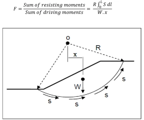
Figure 1.2 illustrates a definition for the factor of safety based on moment equilibrium assuming there is no pore pressure. The resisting shear force acting on the failure surface generates a counter clockwise moment around the center of rotation O with a lever arm equal to the radius of the failure surface R. The weight of the sliding mass generates a clockwise moment with a lever arm equal to x. The factor of safety in terms of moment equilibrium analysis is determined as the ratio of the sum of resisting moments to the sum of driving moments. The resistance moments are computed by integrating on the failure surface the
product of the shear strength and the radius. Equation 1.4 gives the factor of safety based on moment equilibrium for the example presented on Figure 1.2:
=
=
. (1.4)
Figure 1.2 Concept of factor of safety based on moment equilibrium analysis Adapted from Abramson (2002)
1.1.2 Main limit equilibrium methods
1.1.2.1 Swedish method
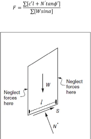
The first method of slices was developed by Fellenius (1936). It divides the length of the sliding mass into several slices. The Swedish method ignores both the normal and shear inter-slice forces (Figure 1.3). The effective normal force N’ at the base of the slice is determined by subtracting the force due to pore pressure (ul, where l is the slice base length) from the component of the weight perpendicular to the slice base (Wcos(α)):
′= − (1.5)
The method takes into account moment equilibrium. The factor of safety in the ordinary method is expressed as follows:
=∑ ′ +
′ ′
∑ (1.6)
Figure 1.3 Slice with forces considered in the Swedish method of slices Adapted from Duncan & Wright (2005)
1.1.2.2 Bishop method
The Bishop method considers inter-slice normal forces and ignores inter-slice shear forces (Abramson, 2002). The forces on both sides of each slice (Ei and Ei+1) are assumed to be
verifying the equilibrium of their vertical component with the weight of the soil in the slice (W):
+ S sin − = 0 (1.7)
Figure 1.4 Slice with forces for Simplified Bishop procedure Adapted from Duncan & Wright (2005)
The mobilized shear stress is calculated as the ratio of the shear strength calculated from the effective normal force N’ and the Mohr-Coulomb parameters, and the factor of safety. The overall factor of safety is obtained by dividing the sum of moments due to the shear strength by the sum of moments due to the soil weight. The factor of safety value is present on both sides of equation 1.8. = ∑ ∆ + − ∆ + / ∑ (1.8)
Therefore, the factor of safety must be obtained by an iterative procedure. In order to calculate the factor of safety by the Bishop Method, a guess value of F must be assumed and used to compute a new F value with Equation 1.8. This process is repeated until convergence
is reached (GEO-SLOPE International). The simplified Bishop’s method is recommended for the analysis of circular failure surfaces (Abramson, 2002).
1.1.2.3 Morgenstern and Price method
Both the Swedish and Bishop methods are based on moment equilibrium alone. The Morgenstern & Price (1965) method allows both the force and moment equilibrium conditions to be verified. It also assumes inclined inter-slice forces for both sides (Figure 1.5). A function f(x) needs to be assumed to describe the direction of inter-slice normal force
E and inter-slice shear force X with respect to the x direction. The various shear-to-normal
ratios along the slip surface are the values of at each slice (Abramson, 2002). Equation 1.9 is proposed by the authers based on assumed function and ratio between inter-slices normal and shear forces to assess stability of slopes. The Morgenstern & Price method allows specifying different types of inter-slice force functions such as constant and half-sine functions. Factor of safety is calculated for both force and moment equilibrium.
= (1.9)
Figure 1.5 Distribution of slice forces for the Morgenstern-Price method Adapted from Duncan & Wright (2005)
1.2 Finite element and finite difference methods
A soil mass is exposed to different loads such as the soil weight and external loads. These loads result in stresses and strains in the soil mass that increase the probability of slope instability. The stress distribution is influenced by the stress-strain properties of the different soil materials (Kondner, 1963). Assumed stress distributions for the limit equilibrium methods presented in section 1.1 vary. Slope stability methods based on finite element stress and strain analyses allow some of the hypotheses behind the limit equilibrium methods to be eliminated. Several slope stability methods based on FEM stresses were developed in the 1980s and 1990s (Matsui & San, 1992). Three main methods are presented in the following sections: the gravity method, the strength reduction method, and stress-based limit-equilibrium methods. As with the limit-limit-equilibrium methods presented in section 1.1, finite-element and finite-difference methods also allow a factor of safety to be calculated.
The concept of finite element analysis depends on a discretization of the slope body into small elements (Figure 1.6). The slope body is assumed to represent a continuum whose mechanical behaviour (e.g. linear elastic) is described by sets of partial differential equations. Displacements, stresses, and strains at nodes in the domain are obtained with the finite element analysis. Once the displacements are obtained, deformations and stresses x, y, and,
xy can be calculated. Finite element and finite difference methods for slope stability
Figure 1.6 Discretization of slope into finite elements by SIGMA/W
1.2.1 Gravity increase method
The gravity increase method GIM consists in increasing the slope mass until the slope fails and an equilibrium state cannot be achieved. The critical slip surface is reached by increasing the gravity gradually with no change in material properties. The increasing gravity glimit is
defined as the product of the rate of gravity increase with respect to time g’ and a parametric time variable limit:
= ′. (1.10)
The gravity increase method defines failure as the highest time value where the loading due to the acceleration of gravity brings strength of slope to the failure merge (Swan & Seo, 1999). The failure in GIM is based on the rate of displacement and damage within the elements during the analysis of finite element. The critical slip surface is formed when the
highest gravity level is reached which causes the largest deformation before failure state (Li et al., 2009). The factor of safety can be defined as the ratio between the critical acceleration of gravity at failure glimit and the real acceleration of gravity gactual equal to 9.81 m/s2.
= (1.11)
1.2.2 Shear strength reduction method
The shear strength reduction method (SRM) was first proposed by Matsui & San (1992). The method was applied by these authors in the 1980s and 1990s for embankment and excavation slopes. Their results proved that this method can be used to evaluate the stability of both types of slopes. Since then, other authors have applied this method (Donald & Giam 1988; Ugai & Leshchinsky 1995; Griffiths & Lane 1999).
With this technique, the slope’s shear strength parameters, its effective cohesion and its friction angle, are progressively reduced until failure occurs. A series of strength reduction factors (SRF) are used to divide the real shear strength parameters. The factor of safety in the SRM is defined as the ratio between the real shear strength parameters to the critical shear strength parameters that lead to failure.
= ℎ
ℎ (1.12)
Failure in the shear strength reduction method is defined as the point where deformations begin to increase rapidly with increasing strength reduction factor values. Shear strength parameters are typically obtained from the Mohr-Coulomb criteria and are reduced incrementally by increasing the SRF:
= ′
′ =
′
where c’reduced is the reduced cohesion value and ϕ’reduced is the reduced friction angle value.
Since the method is based on finite element analysis, it can be adapted to conduct probabilistic analyses of slope stability. A probabilistic analysis is based on defined random variables (cohesion and friction angle) of the slope material. The analysis uses the mean value of the probabilistic values. The conjunction between shear strength reduction method and probabilistic analyses allows SRM to use the random values for assessing slope stability. The results of the coupled analysis are probability failure values, critical strength reduction factor (mean value) and standard deviation values for the critical strength reduction factor.
The strength reduction method has several advantages:
1. An arbitrary slip surface geometry (e.g., circular slip surface) does not have to be assumed;
2. Assumptions regarding inter-slice shear forces are not required;
3. The SRM method is more suitable for complicated conditions (e.g., large-scale slopes of complex geometry);
4. This method gives information about the stress and pore pressure in the soil mass;
5. The displacement depends on strength parameters, such as the soil or rock cohesion and friction angle, but it also depends on their stress-strain properties (E, ν) (Cheng & Wei, 2007).
The SIGMA/W software can be used to compute values of the factor of safety based on SRM. Several SRF values are tested in order to get reduced values of c’ and φ’. The new
values are applied in the finite element model to calculate displacements until a critical value is reached. The SRF then gives the F value (GEO-SLOPE International Ltd, 2007).
1.2.3 Limit equilibrium methods based on finite-element stress
The limit equilibrium methods that have been presented in section 1.1 do not include a stress and strain analysis of the slope materials. According to Bishop (1952), the stresses that are
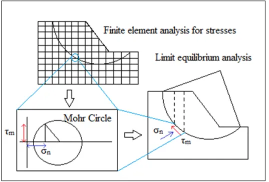
assumed for limit equilibrium analyses do not always correspond to the actual stress in the field. With limit equilibrium methods based on finite element stresses, the stress and strain in the soil mass are computed. The FE stress field is rotated to calculate the shear and normal stress components on the failure surface. The normal and shear stress components and the Mohr-Coulomb parameters allow a ratio between resisting shear forces Sr and mobilized
shear forces Sm to be calculated. Figure 1.7 shows the main steps of limit equilibrium
analyses based on FE stresses.
Figure 1.7 Stresses calculated by FEA and used in a limit equilibrium analysis Adapted from Fredlund et al. (1999)
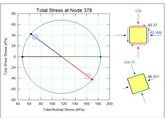
The Mohr circle and its equations are used to find the normal and shear stress components on the failure surface from x, y, and, xy (Figure 1.8). The rotation angle is
calculated from the slip surface inclination.
The shear strength Sr and mobilized shear stress Sm are calculated from equations 1.14 and
= ′ + ′ (1.14)
= (1.15)
The shear strength and mobilized shear stress must be converted to forces by multiplying the stress values with the base length of the slice. The factor of safety (F) is obtained by summing the resisting and mobilized forces and by comparing them:
= ∑ ∑
(1.16)
Figure 1.8 Example of Mohr circle to calculate the normal and shear stresses in SIGMA/W
A large array of tools can be used to calculate the stress in a slope body. For instance, SIGMA/W can be used to compute ground stresses. Figure 1.9 shows an example of vertical stress values obtained with SIGMA/W. These stresses can be transferred to SLOPE/W to calculate F values for a series of slip surface.
Figure 1.9 Vertical stress contours calculated by SIGMA/W
1.2.3.1 Procedure for limit equilibrium analyses based on finite-element stress
The procedure for limit equilibrium analysis based on a finite element stress analysis was presented by Krahn (2003). The main steps can be summarized as follows:
1. A FE code is used to calculate the ground stresses σx, σy, and τxy at the base of each slice;
2. The inclination of the base of each slice (α) is used to rotate the stress components. The rotation is conducted using the Mohr circle and its equations to get the normal and shear stress components at the base of each slice;
3. Equation 1.14 is used to calculate the shear strength at the base of each slice;
4. The resisting and mobilized shear forces are calculated by multiplying the mobilized shear stress and the shear strength at the base of each slice by its base-length (L) to convert stresses to forces;
5. This procedure is repeated for each slice to obtain the total available resisting force and mobilized shear force;
6. The factor of safety is obtained by dividing the total available resisting force by the total mobilized shear force (equation 1.16);
7. Steps 2 to 6 are repeated for different slip surfaces. The critical slip surface will result in the lowest factor of safety.
1.2.3.2 Advantages of using finite element stress method in limit equilibrium analysis
Using FEM stresses for limit equilibrium analyses has many advantages. One of the main challenges with limit equilibrium methods is to define the normal and shear stresses at the base of each slice. These stresses can easily be computed with a finite element analysis.
Figures 1.10 and 1.11 compare the normal stress distributions calculated from a finite-element analyses with SIGMA/W (curves labelled F.E.) with the normal stress distributions assumed with the Morgenstern-Price method (curves labelled L.E.) for two slip surfaces (Krahn, 2003). Figure 1.10 shows the stress distribution for a slip surface that goes through the slope toe. The normal stress values are similar for both methods near the slope crest. Starting from slice 7, a gap develops between the finite-element and Morgenstern-Price normal stresses. The normal stresses become approximately constant for FEM from slice 22 to slice 27. For the Morgenstern-Price method, the normal stress decreases after slice 22. Figure 1.11 shows the normal stress distribution for a deeper slip surface. In this case, the normal stress values for FEM and the Morgenstern-Price method are similar, thus indicating that classical limit-equilibrium methods can be based on adequate normal stress values for some slip surfaces.
Figure 1.9 Distribution of the normal stresses along the toe slip surface Adapted from Krahn (2003)
Figure 1.10 Distribution of the normal stresses along a deep slip surface Adapted from Krahn (2003)
Limit equilibrium analyses based on finite element stresses have the following advantages:
1. FEM stresses are not based on assumed inter-slice forces;
2. The factor of safety is computed based on ground stresses that can be more representative of the real stresses in the field;
3. Dynamic stresses resulting from seismic waves can be considered in the slope stability analyses with FEM methods.
1.3 Slope stability analyses with COMSOL and MATLAB
1.3.1 COMSOL Multiphysics
COMSOL Multiphysics is a computer program based on the finite element method. Its geomechanics and subsurface flow modules allow different geotechnical problems to be studied (e.g., settlements). Unfortunately, COMSOL does not include native tools for slope stability calculations. As a consequence, the literature currently presents very few slope stability analyses based on COMSOL models.
One of the only examples of slope stability analysis based on a COMSOL model was presented by Shao et al. (2014). They used COMSOL to analyse the stability of slopes with a coupled dual-permeability. They computed local values of the factor of safety (Lu et al., 2012). The local factor of safety (LFS) is based on the comparison of the local Mohr-Circle in the slope body with a Mohr-Coulomb criterion. The local factor of safety is defined as a ratio between the shear stress on the failure envelope τ* and the actual shear stress magnitude
τ:
= ∗ (1.17)
The main difference between the local factor of safety and the general factor of safety is that the LFS is computed at individual points of the studied slope but the general factor of safety is computed along a given slip surface for limit equilibrium methods (Zaruba & Mencl, 1982) or is unique for a given slope for strength reduction methods.
Shao et al. (2015) applied linear-elastic behaviour to a fine-grained slope to obtain the stresses. Their local factor of safety values were influnced by the rainfall rate and pore water-pressure. This influence was observed to depend on the soil preoperies. The instability of the slope increases with increasing pore pressures.
1.3.2 MATLAB
New tools for COMSOL can be programmed using the MATLAB LiveLink, a MATLAB programming interface for COMSOL. MATLAB is a programming language for scientific computing. MATLAB has been used separately from COMSOL for a large number of geotechnical applications, such as determining the principal stresses in rock and soil and determining the hydraulic parameters during pumping tests (Zúñiga et al., 2007). Independently from COMSOL, MATLAB was used by Zeng et al. (2009) to conduct slope stability analyses. They used an algorithm to search for the most critical slip surface for slopes.
1.4 Objectives
As previously mentioned, COMSOL does not include a slope stability module. The main objective of this project was to program and validate a limit equilibrium module for COMSOL. This module was to be based on finite-element stresses obtained with COMSOL Multiphysics. The second objective was to verify this new module with the Geo-Studio software package. To our best knowledge, this thesis presents the first example of limit equilibrium analysis with COMSOL.
CHAPTER 2 METHODOLOGY
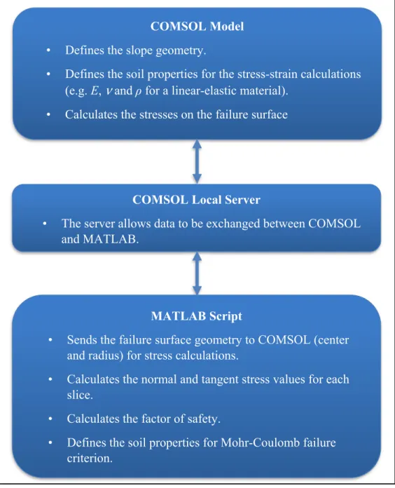
The main objective of this thesis was to program a MATLAB script to conduct slope stability analyses for COMSOL models. COMSOL was used to define the slope geometry and to calculate the stresses in the slope body. MATLAB was used to set the failure surface parameters in COMSOL, to calculate the normal and tangent stress components with respect to the failure surface from the raw x and y stresses calculated in COMSOL, and to calculate the factor of safety for each failure surface. Figure 2.1 shows a schematic representation of the three main components of the COMSOL-MATLAB module.
The current version of the MATLAB script has some important limitations. First, it only allows circular failure surfaces to be tested. Second, it only supports materials with Mohr-Coulomb failure criteria. Third, it only allows three soil layers with different properties to be included in the geometry. The MATLAB script could however easily be modified to conduct more complex analyses.
The MATLAB script was verified using a similar stress-based method programmed in SLOPE/W. In this case, SLOPE/W performs the limit equilibrium analysis while SIGMA/W calculates the stresses and deformations in the slope body (Krahn, 2003). The SLOPE/W model was used to verify the factor of safety for identical sets of failure surfaces. SIGMA/W was used to verify the stress values calculated in COMSOL and rotated in MATLAB. Four slopes with different geometries and layering were used for the verification.
Figure 2.1 A schematic representation of the three components of the COMSOL-MATLAB slope stability module
COMSOL Model
• Defines the slope geometry.
• Defines the soil properties for the stress-strain calculations (e.g. E, ν and ρ for a linear-elastic material).
• Calculates the stresses on the failure surface
COMSOL Local Server
• The server allows data to be exchanged between COMSOL and MATLAB.
MATLAB Script
• Sends the failure surface geometry to COMSOL (center and radius) for stress calculations.
• Calculates the normal and tangent stress values for each slice.
• Calculates the factor of safety.
• Defines the soil properties for Mohr-Coulomb failure criterion.
2.1 COMSOL model
COMSOL version 5.2 was used in this study. In the COMSOL 2D model, the solid mechanics interface was used to calculate displacements, stresses and strains inside the slope model. This stress-strain analysis is based on Navier’s equation. Plane strain and linear-elastic soil behaviour are assumed. The linear-linear-elastic behaviour is based on three main parameters: Young’s modulus E, Poisson’s ratio ν, and soil density ρ.
The COMSOL model includes only one main object (Figure 2.2): the slope body. It is based on a polygon or a series of polygons if the soil is layered.
The same boundary conditions were used in all the slope models that were tested. Free displacements were specified at the surface. Horizontal displacements are fixed at the left and right sides of the model. The bottom of the model has fixed horizontal and vertical displacements. The MATLAB code can handle different boundary conditions.
Gravity was applied to the slope body in the negative y-direction as a force per unit volume. The MATLAB code allows other forces to be added in the COMSOL model (e.g., influence of heat transfer on stress).
A COMSOL server is needed to integrate COMSOL with MATLAB. The server allows COMSOL to be integrated in MATLAB scripts or JAVA classes (e.g. Pirnia et al. 2016). When conducting slope stability analyses, both the COMSOL mph-file and MATLAB script should be in the same directory. The COMSOL server must be launched before the MATLAB script.
Figure 2.2 Slope geometries defined in the COMSOL model
The following steps must be followed when defining the COMSOL model. Figure 2.3 shows these steps as shown in COMSOL software.
1. The model geometry is defined. A polygon interface is used to define the slope body. The input for this interface is the x and y coordinates for all points that form the slope geometry;
2. The parameters for the physics interface of the slope are defined. Linear-elastic material properties are defined. These properties include Young’s modulus, Poisson’s ratio, and density. Boundary conditions and body loads are defined. In case of layered slopes, other linear-elastic materials are created;
Slope body
σy (kPa)
Horizontal displacements fixed at the left and right
Horizontal and vertical displacements fixed at bottom (m)
(m
3. A new mesh sequence is created. A user-controlled mesh is built automatically. Also the element size parameters and free quad settings are applied;
4. A default solver sequence is defined for a stationary study in order to compute the required stresses.
Figure 2.3 The tree structure identifying the main steps for the COMSOL model creation
Step 2
Step 4 Step 3
2.2 MATLAB script
The MATLAB script was used to define the parameters describing the slip surfaces, to define the Mohr-Coulomb parameters of the slope material for uniform or layered slope, to define a number of slices, to define the slope geometry, to import the finite element stresses from COMSOL, to calculate the normal and shear stresses along the failure surface, to compute the shear strength and to compute values of the factor of safety. All these steps will be explained in more details in this section. The MATLAB code is presented in Appendix I.
The parameters describing the slip surfaces, Mohr-Coulomb criteria, number of slices and slope geometry are defined in the first section of the script. The slip surface in the current analysis is assumed to be circular. The x and y coordinates of the center, and the failure surface radius values are defined in three vectors. Soil properties (cohesion and friction angle) are defined in vectors. The number of slices inside the failure wedge is defined. These slices are used to integrate the stress to calculate the factor of safety. A matrix (variable
SlipCircles) of all possible combinations of the three vectors components is built to define n
slip surfaces for which the factor of safety will be calculated. The same matrix is used later in the script to store the factor of safety values. The geometry of the slope body is defined using the x-y coordinates of a polygon or a series of polygons if the soil is layered.
In the second section of the script, a COMSOL file is opened by the MATLAB script. The filename is stored in a string that can be changed by the user. The COMSOL file must be in the same directory as the MATLAB script. The code lines that follow allow points to be defined for the stress interpolation. The variables to be evaluated for these points are also defined (σx, σy, τxy). The finite element equations are then solved. They only need to be
solved once per simulations. The finite element stresses for the different slip circles are interpolated from the same finite element simulation.
Section three of the script contains a loop (for loop) that allows the factor of safety to be calculated for all slip surfaces. Inside the loop, the coordinates of a series of points on the
failure circle are computed using the radius and the trigonometric circle parametrization. Once the slip circle is defined, the intersection points between the circle and the slope geometry are computed using the polyxpoly function. Normally, two intersection points are found for suitable slip circles. Incorrect circles either do not touch the slope body or have more than two intersection points (special case in benched slope). The script moves to the next for loop iteration without calculating a factor of safety for these two cases.
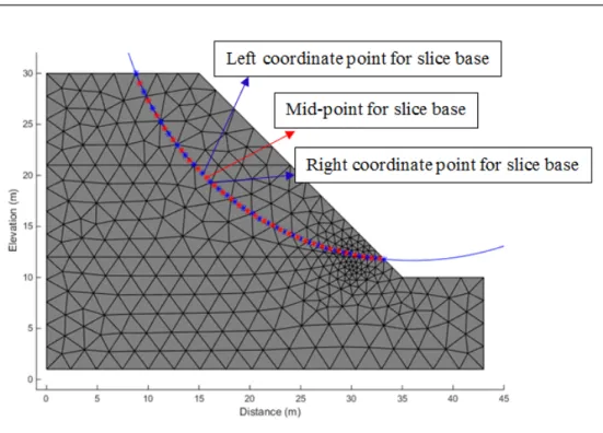
For correct slip surfaces, the two extreme x values of the intersection points are used to define the limit of the soil wedge inside the slip surface. The slice width is calculated from the difference between the two extreme x values. The x-coordinates of the slice bases are then calculated based on the slice width. The y-coordinates are based on x-coordinates of the slice base and the failure circle equation. Finally, mid-points xm and ym (red points) at the base of
each slice are computed based on left and right coordinates xb and yb (blue points) at the base
of each slice (Figure 2.3). These points are the locations where the finite element stresses should be computed.
Section four of the script contains code lines to extract the stress values at the mid-point of the base of each slice from the COMSOL model. The COMSOL model interpolates σx, σy,
and, τxy from the finite-element solution.
Section five applies to cases where the soil body is composed of more than one layer. The
inpolygon function is used to find in which layer the points are located and to assign the
proper c’ and ’ values in vectors describing the Mohr-Coulomb parameters for the base of each slice.
The inclination angle α of each slice base is computed in section six and using next equation.
α = tan-1
(2.1)
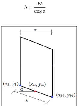
The actual base length (b) of the slice is determined by using the inclination angle of each slice and the slice width (w):
=
cos α (2.2)
Figure 2.5 Illustrates the coordinates of slice base, horizontal slice width (w), slice base inclination (α) and actual slice base length (b)
In section seven, the stress components imported from COMSOL are rotated to calculate the normal σn and shear τn stresses at the center point of the slice base (xm, ym) using equation 2.3
and 2.4 respectively:
= + /2 + – /2 cos 2 + sin 2 (2.3)
= − − /2 sin 2 + cos 2 (2.4)
Figure 2.6 Illustrates normal and shear stresses at slice base
The normal and shear stresses are used with the soil’s Mohr-Coulomb parameters to calculate the shear strength along the slice base:
Shear strength = + tan (2.5)
The mobilized shear stress corresponds to the shear stress along the slice base:
The shear strength and mobilized shear stress must be converted into forces by multiplying the stresses by the base length (b). The forces are then summed:
Resistance shear forces = + tan (2.7)
Mobilized shear forces = (2.8)
The final step consists in computing the factor of safety (F):
F =Resistance shear forces Mobilized shear forces =
∑ + tan
∑ (2.9)
Figure 2.4 explains schematically the main steps of the factor of safety calculations with COMSOL and the MATLAB script.
Figure 2.7 Schematic representation of the COMSOL-MATLAB script used to compute the factor of safety
Running COMSOL multiphysics
MATLAB
Simulate slope models using E, ν, and ρ
Solve FEA to compute σx, σy, and, τxy
Running COMSOL server
Defines;
x, y, R parameters for slip surface x-y coordinates for slope model c’ and ϕ’for soil properties
for loop to test all failure surfaces and determine xm and ym
COMSOL model is open in MATLAB script
Import FEA stresses
If: 2 layers or more
Compute resistance and mobilized forces Find α, σn, and, τn
Uses in-polygon function to find x, y, c’, and ’ [in] and x, y, c’, and ’ [out] If: 1 layer
Calculate F MATLAB
2.3 GEO-SLOPE model
To verify the MATLAB script and the COMSOL model, a series of slope stability calculations were conducted with two modules from the GEO-SLOPE suite of software. The first module was SIGMA/W. It uses the FEM to compute the stress distribution in slopes based on the soil’s E, ν and ρ. The second tool is SLOPE/W, it uses LEM equations to calculate the factor of safety based on the soil’s c’ and ’, and the FEM stresses.
Figure 2.5 shows the distribution of vertical stresses in the first slope used for code verification (uniform slope). The geometry and soil properties were based on Krahn (2003). The second, third, and fourth slopes are respectively benches, a steep slope, and a uniform slope in a layered soil deposit. The same stress-strain and Mohr-Coulomb parameters were used for each slope, except for the layered soil deposit for which different parameters were used.
Figure 2.8 Distribution of vertical stresses in the uniform slope model using SIGMA/W
The same four models were created in COMSOL and MATLAB in order to compare the results with the GEO-SLOPE models. These four models and their results will be described in detail in the following chapter.
CHAPTER 3
CODE VERIFICATION RESULTS AND DISCUSSION
The stability of slopes with different geometries and soil properties was analyzed using the COMSOL-MATLAB module introduced in the previous chapter and the stress-based method available with SLOPE/W and SIGMA/W in the GEO-SLOPE software package. Four slopes were tested: a uniform slope, a slope with benches, a steep slope, and a slope in a layered soil deposit. For each slope, the factor of safety was calculated for a series of failure surfaces. Code verification with SLOPE/W was carried out using the same slope, the same properties and the same failure surfaces. The MATLAB code programmed for this study is presented in Appendix I.
The chapter presents the results of this verification. The comparison is focused on finite element stresses and the factor of safety. A detailed comparison of finite element stresses and comparison of numerical results of finite element stresses are presented in Appendix II. The comparison of factor of safety values with graphs are presented in Appendix III.
3.1 Analysis of COMSOL-MATLAB and GEO-SLOPE models
3.1.1 Analysis of uniform slope
The uniform soil model has a height of 30 m and length of 43 m with slope height and length of 20 m (Figure 3.1). This corresponds to an inclination of 45o. The soil has a unit weight of
18 kN/m³. Linear-elastic behaviour was assumed for the finite element analysis in COMSOL and SIGMA/W with a Young’s modulus of 1 GPa and a Poisson’s ratio of 0.3. Cohesion and friction angle of respectively 5 kPa and 20o were assumed based on Krahn (2003). Pore
Figure 3.1 Distribution of σy in uniform slope computed with COMSOL with slip surface
and lowest factor safety computed with MATLAB
With both MATLAB and SLOPE/W, the analysis was conducted using 30 slices. A total of 20 slip surfaces were used. The slip surfaces were specified in GEO-SLOPE using a grid for the slip surface centers and a set of slip surface radiuses. The same center coordinates and radiuses were used in the MATLAB script.
Figures 3.2 presents a comparison of the vertical finite element stresses (σy) obtained with
COMSOL and SIGMA/W on the failure surface shown in Figure 3.1. The lowest σy values
correspond to the top of the slope and the exit point of the failure surface at the bottom of the slope. The vertical stress reaches 157 kPa at slice 14. The results obtained with COMSOL and SIGMA/W are nearly identical with a maximum difference of 2 kPa. Horizontal σx and
Slip surface in uniform slope with lowest F =
tangent τxy stresses are also almost identical for this slope geometry with a maximum
difference of 1 and 2 kPa respectively (Appendix II).
The MATLAB code presented in Appendix I divide the sliding mass in equal-width slices. This is not the case in SLOPE/W where the slope width can sometime vary slightly depending on the slope geometry. This has an impact on the location of the slice base mid-point and inclination.
Figure 3.2 Comparison of σy between COMSOL and SIGMA/W
for the uniform slope
Information on the slip surface with the lowest F obtained with the MATLAB code and SLOPE/W for the uniform slope is presented in table 3.1. As shown in the table, the same surface produced the lowest F value for both MATLAB and SLOPE/W.
Figure 3.3 shows the factor of safety values that were obtained with SLOPE/W and COMSOL-MATLAB. The analysis was done for 20 slip surfaces, but only 17 slip surfaces allow computing a factor of safety. The other 3 slip surfaces did not allow a factor of safety to be calculated because they crossed the vertical boundaries of the domain. SLOPE/W also
0,0 25,0 50,0 75,0 100,0 125,0 150,0 175,0 8,0 10,0 12,0 14,0 16,0 18,0 20,0 22,0 24,0 26,0 28,0 30,0 32,0 σy (kPa) x (m) σy-Geostudio σy-COMSOL
detected these slip surfaces. In Figure 3.3, the red line shows the results of GEO-SLOPE and COMSOL-MATLAB if both are completely identical and the blue line is the obtained results. The F values vary between 0.717 (critical value) and 1.713 for COMSOL-MATLAB code and between 0.718 (critical value) and 1.696 for SLOPE/W. The linear regression has a slope of 1.0242 and an intercept of -0.0141. It indicates that SLOPE/W and COMSOL-MATLAB gave similar F values. Detailed results of factor of safety for the 20 slip surfaces are given in Appendix III.
Table 3.1 COMSOL-MATLAB and SLOPE/W results for slip surface with the lowest F for uniform slope
Slip surface with lowest F for uniform slope
Tool Failure circle coordinates Radius Sum of resistance forces Sum of mobilized forces Factor of safety X (m) Y (m) R (m) Sr (kN) Sm (kN) F COMSOL- MATLAB 34 40 26.877 905.53 1260.81 0.718 GEO-SLOPE 34 40 26.877 904.85 1262.28 0.717
Figure 3.3 Comparison between obtained and ideal factor of safety values with SLOPE/W and COMSOL for the uniform slope
3.1.2 Analysis of slope with benches
The height and length of the slope are 30 m and 24 m respectively (Figure 3.4). The slope consists of two benches with different inclinations. The soil conditions are identical to the uniform slope. Pore pressures were also not considered in the analysis. The analysis was conducted with 30 slices. The same 20 slip surfaces were used in SLOPE/W and the MATLAB script. y = 1,0238x - 0,0142 R² = 0,9999 0,6 0,7 0,8 0,9 1,0 1,1 1,2 1,3 1,4 1,5 1,6 1,7 1,8 0,6 0,7 0,8 0,9 1,0 1,1 1,2 1,3 1,4 1,5 1,6 1,7 1,8 Factor of Safety by COMSOL
Factor of Safety by GeoStudio Obtained results
Dashed line for theoretical 1:1 results
Figure 3.4 Distribution of σy in slope with benches computed with COMSOL with slip
surface and lowest F computed with MATLAB
A comparison of the vertical stresses along the slip surface for the COMSOL and SIGMA/W finite element analyses is shown in Figure 3.5. The lowest σy values are concentrated at the
top of the slope. The stress values for COMSOL and SLOPE/W start at x = 9.747 m to x = 13.206 m with the same values. After x = 13.206 m they began to diverge smoothly toward the exit of the slip surface at the bottom of the slope. The finite element stresses of the benches slope presented in (Appendix II).
Slip surface with lowest F = 0.402
Figure 3.5 Comparison of σy between COMSOL and SIGMA/W for
slope with benches
Table 3.2 shows the parameters of the slip surfaces with the lowest F value that were obtained with the MALTAB code and SLOPE/W for the slope with benches. Both codes identified the same slip surface with similar F values.
The part of the code where the validity of the slip surfaces is verified faces a different challenge with this slope as some slip surfaces intersect the slope at more than two points (Figure 3.4). The factor of safety is computed for the sliding mass between the first and second intersection points for both SLOPE/W and MATLAB code.
Figure 3.6 shows the factor of safety values that were obtained with SLOPE/W and COMSOL-MATLAB for 20 slip surfaces. The F values vary between 0.402 and 1.186 for the COMSOL-MATLAB code and between 0.403 and 1.216 for SLOPE/W. The linear regression shown in Figure 3.3 with a slope of 0.9605 and an intercept of 0.0201 indicates that SLOPE/W and COMSOL-MATLAB gave similar F values.
-20,0 0,0 20,0 40,0 60,0 80,0 100,0 120,0 140,0 160,0 180,0 200,0 220,0 9,5 10,0 10,5 11,0 11,5 12,0 12,5 13,0 13,5 14,0 σy (kPa) x (m) σy-Geostudio σy-COMSOL
Table 3.2 COMSOL-MATLAB and SLOPE/W results for slip surface with the lowest F for the slope with benches
Critical slip surface for benches slope
Tool Failure circle coordinates Radius Sum of resistance forces Sum of mobilized forces Factor of safety X (m) Y (m) R (m) Sr (kN) Sm (kN) F COMSOL- MATLAB 36 47 27.511 100.58 250.17 0.402 GEO-SLOPE 36 47 27.511 101.485 251.627 0.403
Detailed results for the 20 slip surfaces are given in Appendix III. All slip surfaces are passing through the slope body, so factor of safety were computed for all slip surfaces. In Figure 3.6, the obtained results line and the ideal results line are almost identical with a very small gap.
Figure 3.6 Comparison between obtained and ideal factor of safety values with SLOPE/W and COMSOL slope with benches
3.1.3 Analysis of steep slope
The steep slope has a height of 22 m and a length of 8 m (Figure 3.7). The soil properties for this example are identical to the previous examples. The analysis did not take into account pore pressures. As with the previous examples, 20 slip surfaces were compared. Each slip surface was analysed with 30 slices.
y = 0,9861x - 0,0003 R² = 0,9976 0,3 0,4 0,5 0,6 0,7 0,8 0,9 1,0 1,1 1,2 1,3 0,3 0,4 0,5 0,6 0,7 0,8 0,9 1,0 1,1 1,2 1,3 Factor of Safety by COMSOL
Factor of Safety by Geo-Studio Dashed line for
theoretical 1:1
Figure 3.7 Distribution of σy in steep slope computed with COMSOL with slip surface and
lowest F computed with MATLAB
The σy distributions in both models are once again similar. Figure 3.8 shows σy for the slip
surface with the lowest F value shown in Figure 3.7. The lowest σy values are located at the
crest and they increase toward the bottom of the slip surface. The vertical stress increase at the end of slope to around 165.4 kPa at x = 24.685 m. The difference between the σy values
for COMSOL and SIGMA/W along the failure surface is generally small but it increases slightly at both the entry and exit points of the slip surface. The horizontal σx and tangent τxy
stresses lead to maximum differences of 3 and 4 kPa receptively. The finite element stresses are compared in (Appendix II).
Slip surface with the lowest F value (0.507)
Figure 3.8 Comparison of σy between COMSOL and SIGMA/W in steep slope
The slip surfaces with the lowest F values in COMSOL and SLOPE/W are given in Table 3.3. Once again the same slip surfaces lead to the lowest F values in COMSOL and SLOPE/W.
Table 3.3 COMSOL-MATLAB and SLOPE/W results for slip surface with the lowest F for the steep slope
5,0 20,0 35,0 50,0 65,0 80,0 95,0 110,0 125,0 140,0 155,0 170,0 14,0 15,0 16,0 17,0 18,0 19,0 20,0 21,0 22,0 23,0 24,0 25,0 σy (kPa) x (m) σy-Geostudio σy-COMSOL
Critical slip surface results of steep slope
Tool Failure circle coordinates Radius Sum of resistance forces Sum of mobilized forces Factor of safety X (m) Y (m) R (m) Sr (kN) Sm (kN) F COMSOL- MATLAB 34 40 20.524 398.48 785.53 0.507 GEO-SLOPE 34 40 20.524 399.18 785.13 0.508
Figure 3.9 shows the range of factor of safety values for SLOPE/W and COMSOL-MALTAB code for the 19 slip surfaces. The F values vary from 0.507 to 2.103 for COMSOL-MATLAB and from 0.508 to 2.105 for SLOPE/W. For slip surface number 11, the failure circle goes through the fixed vertical boundaries of the soil body slope. The failure surface was rejected by both the COMSOL-MATLAB code and SLOPE/W. The linear regression for the obtained results has a slope of 1.0009 and an intercept of 0.0049 with y = x and R2 = 1 for the ideal results. Both lines seem to correspond for all F values. It also
indicates that the COMSOL-MATLAB code gave F values that were similar to those of SLOPE/W for the steep slope.
Figure 3.9 Comparison between obtained and ideal factor of safety values with SLOPE/W and COMSOL for steep slope
y = 1,0009x + 0,0049 R² = 0,9998 0,4 0,5 0,6 0,7 0,8 0,9 1,0 1,1 1,2 1,3 1,4 1,5 1,6 1,7 1,8 1,9 2,0 2,1 2,2 0,4 0,5 0,6 0,7 0,8 0,9 1,0 1,1 1,2 1,3 1,4 1,5 1,6 1,7 1,8 1,9 2,0 2,1 2,2 Factor of Safety by COMSOL
Factor of Safety by Geo-Studio
Dashed line for theoretical 1:1 Obtained results
3.1.4 Analysis of slope in layered soil deposit
The slope body consists in three layers. The slope has a height of 20 m and a length of 20 m (Figure 3.10). The inclination of the slope is 45o. The upper and lower layers are silty to
clayey sand with c’ = 5 kPa, φ’ = 31o, and a unit weight of 21 kN/m3. The Young’s modulus
and Poisson’s ratio for this layer were set at 50 MPa and 0.3 respectively. The middle layer was assumed to be clay with c’ = 25 kPa, φ’ = 22o, and a unit weight of 17.5 kN/m3. Its
Young’s modulus and Poisson’s ratio were set to of 20 MPa and 0.4 respectively.
Figure 3.10 Distribution of σy in layered slope computed with COMSOL with slip surface
and lowest F value computed with MATLAB
Slip surface with lowest F (1.033) for the layered
The analysis also was conducted using 20 slip surfaces and 30 slices for both MATLAB and SLOPE/W. The slip surfaces parameters obtained from GEO-SLOPE are used in MATLAB script following the same procedures for the previous models.
Figure 3.11 presents the distribution of vertical stresses along the lowest F failure plane in both COMSOL and SIGMA/W. The minimum values of σy correspond to the top of the slope
and the end of the failure surface. The vertical stresses start to increase from the top of the slope until the middle at x = 18 m. The stresses then goes down toward the bottom of the slope until x = 32 m.
Figure 3.11 Comparison of σy between COMSOL and SIGMA/W
for layered soil deposit -15,0 5,0 25,0 45,0 65,0 85,0 105,0 125,0 145,0 165,0 185,0 8,0 10,0 12,0 14,0 16,0 18,0 20,0 22,0 24,0 26,0 28,0 30,0 32,0 34,0 σy (kPa) x (m) σy-Geostudio σy-COMSOL