HAL Id: hal-01027582
https://hal.inria.fr/hal-01027582
Submitted on 26 Mar 2015
HAL is a multi-disciplinary open access
archive for the deposit and dissemination of
sci-entific research documents, whether they are
pub-lished or not. The documents may come from
teaching and research institutions in France or
abroad, or from public or private research centers.
L’archive ouverte pluridisciplinaire HAL, est
destinée au dépôt et à la diffusion de documents
scientifiques de niveau recherche, publiés ou non,
émanant des établissements d’enseignement et de
recherche français ou étrangers, des laboratoires
publics ou privés.
A Principled Way of Assessing Visualization Literacy
Jeremy Boy, Ronald A. Rensink, Enrico Bertini, Jean-Daniel Fekete
To cite this version:
Jeremy Boy, Ronald A. Rensink, Enrico Bertini, Jean-Daniel Fekete. A Principled Way of Assessing
Visualization Literacy. IEEE Transactions on Visualization and Computer Graphics, Institute of
Elec-trical and Electronics Engineers, 2014, 20 (12), pp.10. �10.1109/TVCG.2014.2346984�. �hal-01027582�
A Principled Way of Assessing Visualization Literacy
Jeremy Boy, Ronald A. Rensink, Enrico Bertini, and Jean-Daniel Fekete Senior Member, IEEE Abstract— We describe a method for assessing the visualization literacy (VL) of a user. Assessing how well people understand visualizations has great value for research (e. g., to avoid confounds), for design (e. g., to best determine the capabilities of an audience), for teaching (e. g., to assess the level of new students), and for recruiting (e. g., to assess the level of interviewees). This paper proposes a method for assessing VL based on Item Response Theory. It describes the design and evaluation of two VL tests for line graphs, and presents the extension of the method to bar charts and scatterplots. Finally, it discusses the reimplementation of these tests for fast, effective, and scalable web-based use.Index Terms—Literacy, Visualization literacy, Rasch Model, Item Response Theory
1 INTRODUCTION
In April 2012, Jason Oberholtzer posted an article describing two charts that portray Portuguese historical, political, and economic data [36]. While acknowledging that he is not an expert on these top-ics, Oberholtzer claims that thanks to the charts, he feels like he has “a well-founded opinion on the country.” He attributes this to the simplic-ity and efficacy of the charts. He then concludes by stating: “Here’s the beauty of charts. We all get it, right?”
But do we all really get it? Although the number of people famil-iar with visualization continues to grow, it is still difficult to estimate anyone’s ability to read graphs and charts. When designing a visual-ization for non-specialists or when conducting an evaluation of a new visualization system, it is important to be able to pull apart the po-tential efficiency of the visualization and the actual ability of users to understand it.
In this paper, we focus on building a set of visualization liter-acy(VL) tests for line graphs, bar charts, and scatterplots. At this point, we loosely define visualization literacy as the ability to use well-established data visualizations (e. g., line graphs) to handle informa-tion in an effective, efficient, and confident manner.
To generate these tests, we develop here a method based on Item Response Theory (IRT). Traditionally IRT has been used to assess ex-aminees’ abilities and other psychological constructs via predefined tests and surveys in areas such as education [27], social sciences [15], and medicine [32]. Here, we first use IRT in a design phase to evaluate the relevance of potential test items. We then use it in an assessment phasefor measuring a user’s level of visualization literacy. Finally, based on these measures, we develop a series of tests for fast, effec-tive, and scalable web-based use. The great benefit of this method is that inherits IRT’s property of making ability assessments that are based not only on raw scores, but on a model that captures the stand-ing of users on latent traits (e. g., the ability to use various graphical representations).
As such, our main contributions are as follows: • a definition of visualization literacy,
• a method for: 1) assessing the relevance of VL test items, 2) assessing an examinee’s level of visualization literacy, 3) making
• Jeremy Boy is with Inria, Telecom ParisTech, and EnsadLab. E-mail:
• Ronald A. Rensink is with the University of British Columbia. E-mail:
• Enrico Bertini is with NYU Polytechnic School of Engineering. E-mail:
• Jean-Daniel Fekete is with Inria. E-mail: [email protected].
Manuscript received 31 March 2013; accepted 1 August 2013; posted online 13 October 2013; mailed on 4 October 2013.
For information on obtaining reprints of this article, please send e-mail to: [email protected].
fast and effective assessments of visualization literacy for well established visualization techniques and tasks; and
• an implementation of four online tests, based on our method. Our immediate motivation for this work is to design a series of tests that can help Information Visualization (InfoVis) researchers detect low-ability participants when conducting online studies, in order to avoid possible confounds in their data. This requires the tests to be short, reliable, and easy to administer. However, such tests can also be applied to many other situations, such as:
• designers who want to know how capable of reading visualiza-tions their targeted audience is;
• teachers who want to make a first or final assessment of the ac-quired knowledge of freshmen;
• practitioners who need to hire capable analysts; and
• education policy-makers who may want to set a standard for vi-sualization literacy.
This paper is organized in the following way. It begins with a back-ground section that defines the concept of literacy and discusses some of its best-known forms. Also introduced are the theoretical constructs of information comprehension and graph comprehension, along with the concepts behind Item Response Theory. Section 3 presents the ba-sic elements of our approach. Section 4 shows how these can be used to create and administer two VL tests using line graphs. In Section 5, our method is extended to bar charts and scatterplots. Section 6 describes how our method can be used to redesign fast, effective, and scalable web-based tests. Finally, Section 7 provides a set of “take-away” guidelines for the development of future tests.
2 BACKGROUND
Very few studies investigate the ability of a user to extract information from a graphical representation such as a line graph or bar chart. And of those that do, most make only higher-level assessments: they use such representations as a way to test mathematical skills, or the ability to handle uncertainty [37, 14, 52, 34, 35]. A few attempts do focus more on the interpretation of graphically-represented quantities [23, 21], but they base their assessments only on raw scores and limited test items. This makes it difficult to create a true measure of VL.
2.1 Literacy
2.1.1 Definition
The online Oxford dictionary defines literacy as “the ability to read and write”. While historically this term has been closely tied to its textual dimension, it has grown to become a broader concept. Taylor proposes the following much broader definition: “Literacy is a gate-way skillthat opens to the potential for new learning and understand-ing” [47].
Given this broader understanding, other forms of literacy can be dis-tinguished. For example, numeracy was coined to describe the skills
needed for reasoning and applying simple numerical concepts. It was intended to “represent the mirror image of [textual] literacy” [46, p. 269]. Like [textual] literacy, numeracy is a gateway skill.
With the advent of the Information Age, several new forms of liter-acy have emerged. Computer literliter-acy “refers to basic keyboard skills, plus a working knowledge of how computer systems operate and of the general ways in which computers can be used” [38]. Information liter-acyis defined as the ability to “recognize when information is needed and have the ability to locate, evaluate, and use effectively the needed information” [25]. Media literacy commonly relates to the “ability to access, analyze, evaluate and create media in a variety of forms” [54].
2.1.2 Higher-level Comprehension
In order to develop a meaningful measure of any form of literacy, it is necessary to understand the various components involved, starting at the higher levels. Friel et al. [19] suggest that comprehension of in-formation in written form involves three kinds of tasks: locating, inte-grating, and generating information. Locating tasks require the reader to find a piece of information based on given cues. Integrating tasks require the reader to aggregate several pieces of information. Generat-ing tasksnot only require the reader to process given information but also require the reader to make document-based inferences or to draw on personal knowledge.
Another important aspect of information comprehension is question asking, or question posing. Graesser et al. [20] posit that question posing is a major factor in text comprehension. Indeed, the ability to pose low-level questions, i. e., to identify a series of low-level tasks, is essential for information retrieval and for achieving higher-level, or deeper, goals.
2.1.3 Assessment
Several literacy tests are in common use. The two most impor-tant are UNESCO’s Literacy Assessment and Monitoring Programme (LAMP) [51] and the Organisation for Economic Co-operation and Development (OECD)’s Programme for International Student Assess-ment (PISA) [37]. Other assessments include the Adult Literacy and Lifeskills Survey (ALL) [33], the International Adult Literacy Survey (IALS) [26], and the Miller Word Identification Assessment (MWIA) [31].
Assessments are also made using more local scales like the US Na-tional Assessment of Adult Literacy (NAAL) [3], the UK’s Depart-ment for Education Numeracy Skills Tests [14], or the University of Kent’s Numerical Reasoning Test [52].
Most of these tests, however, take basic literacy skills for granted, and focus on higher-level assessments. For example the PISA test is designed for 15 year-olds who are finishing compulsory education. This implies that examinees should have learned–and still remember– the basic skills required for reading and counting. As such, testing basic literacy skills is irrelevant. It is only when examinees clearly fail these tests that certain measures are deployed to test the lower-level skills.
NAAL provides a set of 2 complementary tests administered to ex-aminees who fail the main Textual literacy test [3]: the Fluency Ad-dition to NAAL (FAN) and The Adult Literacy Supplemental Assess-ment (ALSA). These tests focus on adults’ ability to read single words and small passages.
Meanwhile, MWIA tests whole-word dyslexia. It has 2 levels, each of which contains 2 lists of words, one Holistic and one Phonetic, that examinees are asked to read aloud. Evaluation is based on time spent reading and number of words missed. Proficient readers should find such tests extremely easy, while low ability readers should find them more challenging.
2.2 Visualization Literacy
2.2.1 Definition
The view of literacy as a gateway skill can also be applied to the ex-traction and manipulation of information from graphical representa-tions such as line graphs or bar charts. In particular, it can be the basis
for what we will refer to as visualization literacy (VL): the ability to confidently use a given data visualization to translate questions spec-ified in the data domain into visual queries in the visual domain, as well as interpreting visual patterns in the visual domain as properties in the data domain.
This definition is related to several others that have been proposed concerning visual messages. For example, a long-standing and often neglected form of literacy is visual literacy. This has been defined as the “ability to understand, interpret and evaluate visual messages” [8]. Visual literacy is rooted in semiotics, i. e., the study of signs and sign processes, which distinguishes it from visualization literacy. While it has probably been the most important form of literacy to date, it is nowadays frowned upon; indeed, present-day literacy tests do not take visual literacy into account.
Taylor [47] has advocated for the study of visual information lit-eracy, while Wainer has advocated for graphicacy [53]. Depending on the context, these terms refer to the ability to read charts and di-agrams, or to qualify the merging of visual and information literacy teaching [2]. Because of this ambiguity, we prefer the more general term “visualization literacy.”
2.2.2 Higher-level Comprehension
Bertin [4] proposed three levels on which a graph may be interpreted: elementary, intermediate, and comprehensive. The elementary level concerns the simple extraction of information from the data. The inter-mediate levelconcerns the detection of trends and relationships. The comprehensive levelconcerns the comparison of whole structures, and inferences based on both data and background knowledge. Similarly, Curcio [13] distinguishes three ways of reading from a graph: from the data, between the data, and beyond the data.1
The higher-level cognitive processes behind the reading of graphs has been the concern of the area of graph comprehension. This area studies the specific expectations viewers have for different graph types [50], and has highlighted many differences in the understanding of novices and expert viewers [16, 28, 29, 48].
Several influential models of graph comprehension have been pro-posed. For example, Pinker [39] describes a three-way interaction be-tween the visual features of a display, processes of perceptual organi-zation, and what he calls the graph schema, which directs the search for information in the particular graph. Several other models are sim-ilar (see Trickett and Trafton [49]). All involve the following steps:
1. the user has a pre-specified goal to extract a specific piece of information
2. the user looks at the graph and the graph schema and gestalt pro-cesses are activated
3. the salient features of the graph are encoded, based on these gestalt principles
4. the user now knows which cognitive/interpretative strategies to use, because the graph is familiar
5. the user extracts the necessary goal-directed visual chunks 6. the user may compare 2 or more visual chunks
7. the user extracts the relevant information to satisfy the goal Visual “chunking” consists in segmenting a visual display into smaller parts, or chunks [28]. Each chunk represents a set of entities that have been grouped according to gestalt principles. Chunks can in turn be subdivided into smaller chunks.
Shah [45] identifies two cognitive processes that occur during stages 2 through 6 of this model:
1. a top-down process where the viewer’s prior knowledge of se-mantic content influences data interpretation, and
2. a bottom-up process where the viewer shifts from perceptual pro-cesses to interpretation.
1For further reference, refer to Friel et al.’s Taxonomy of Skills Required for
These processes are then interactively applied to different chunks, suggesting that the interpretation process is serial and incremental. However Carpenter & Shah [9] have shown that graph comprehen-sion, and more specifically visual feature encoding, is rather an itera-tive process than a straight-forward serial process.
Freedman & Shah [17] relate the top-down and bottom-up pro-cesses respectively to a construction and an integration phase. Dur-ing the construction phase, the viewer activates prior graphical knowl-edge, i. e., the graph schema, and domain knowledge to construct a co-herent conceptual representation of the available information. During the integration phase, disparate knowledge is activated by “reading” the graph and is combined to form a coherent representation. These two phases take place in alternating cycles. This suggests that do-main knowledge can influence the interpretation of graphs. However, highly visualization-literate people should suffer less influence of both the top-down and bottom-up processes [45].
2.2.3 Assessment
Relatively little has been done on the assessment of literacy involving graphical representations. However, interesting work has been done on measuring the perceptual abilities of a user to extract information from several types of graphical representations. For example, various studies have demonstrated that users can perceive slope, curvature, di-mensionality, and continuity in line graphs (see [12]). In addition, Correll et al. [12] have shown that users can make judgements about aggregate properties of data using these graphs.
Scatterplots have also received some degree of attention. For exam-ple, studies have examined the ability of a user to determine Pearson correlationr [5, 10, 30, 40, 42]. Several interesting results have been obtained, such as general tendency to underestimate correlation, es-pecially in the range .2< |r| < .6, and an almost complete failure to perceive correlation when |r| < .2.
Concerning the outright assessment of literacy, the only relevant work we know of is Wainer’s study on the difference in graphicacy lev-els between third-, fourth-, and fifth-grade children [53]. In this study, an 8 item test was developed for several visualizations, including line graphs and bar charts. The test was scored using Item Response The-ory [55], which proved to be a very effective way of assessing abilities. The study revealed that children reach “adult levels of graphicacy” as soon as the fourth-grade, leaving “little room for further improve-ment.” However, it is unclear what these “adult levels” are. If we look at textual literacy, some children are more literate than certain adults. People may also forget these skills if they do not regularly practice. Therefore, while very useful, we consider Wainer’s work to be lim-ited. A way to assess adult levels of visualization literacy is necessary.
2.3 Item Response Theory and the Rasch Model
Consider what we would like in an effective VL test. To begin with, it should cover a certain range of abilities, each of which could be measured by specific scores. Imagine such a test has 10 items, which are marked 1 when answered correctly, and 0 otherwise. Rob sits the test and gets a score of 2. Jenny also sits the test, and gets a score of 7. We would hope that this means that Jenny is better than Rob at reading graphs. If both Rob and Jenny were to take the test again, we would also expect that both would get approximately the same scores, or at least that Jenny would still get a higher score than Rob. And we would expect that whatever VL test Rob and Jenny both take, Jenny will always be better than Rob.
Now imagine that Chris sits the test and also gets a score of 2. If we based our judgement on this raw score, we would assume that Chris is as bad as Rob at reading graphs. However, taking a closer look at the items that Chris and Rob got right, we realize that they are different: Rob gave correct answers for the two easiest items, while Chris gave correct answers to two relatively complex items. This would of course require us to know the level of difficulty of each item, and would mean that while Chris gave incorrect answers to the easy items, he might show some ability to read graphs. Thus we would want the different scores to have “meanings,” i. e., it would be nice to be able to predict
whether Chris was simply lucky (he guessed the answers), or whether he is in fact able to get the simpler items right, even though he didn’t this time.
Imagine now that Rob, Jenny, and Chris take a second VL test. Rob gets a score of 3, Chris gets 4, and Jenny gets 10. We would infer that this test is easier, since the grades are higher. However, if we look at the intervals between examinees’ scores, we see that Jenny is 7 points ahead of Rob in this test, whereas she was only 5 points ahead in the first one. If we were to truly measure abilities, we would want these intervals to be invariant. In addition, seeing that Chris’ score is once again similar to Rob’s (knowing that they both got the same items right this time), would lead us to think that they do in fact have similar levels of ability. However, this test actually provides more information on lower abilities, since it was able to differentiate Chris and Rob, while the first test could not.
Finally, imagine that all three examinees take a third VL test. This time, they all get scores of 10. We may conclude that this test is not good for detecting the ability to read graphs. However, another possi-bility would be that all items in this test share the same (low) level of difficulty. This would mean that this test does in fact assess ability to read graphs, but its items are redundant and not very discriminant.
One way of fulfilling all of these requirements is by using Item Re-sponse Theory (IRT) [55]. This is a model-based approach that does not use response data directly, but transforms them into estimates of latent traits (e. g., abilities), which then serve as the basis of assess-ment. IRT models have been applied to tests in a variety of fields such as health studies, education, psychology, marketing, economics, social sciences (see [44]), and even in graphicacy [53].
The core idea is to predict the probability of success of an examinee on an item. This depends on both the examinee’s ability and the item’s difficulty. An important aspect of IRT is that it projects both of these characteristics onto the same scale–that of the latent trait. Ability (or standing on the latent trait) is derived from a pattern of responses to a series of test items. Item difficulty is defined by the 0.5 probability of success of an examinee with the appropriate ability for the item. For example, an examinee with an ability value of 0 (0 being the value attributed to an average achiever) will have a 50% chance of giving a correct answer to an item that has a difficulty value of 0.
IRT offers models for dichotomous (e. g., true/false question re-sponses) and for polytomous data (e. g., responses on likert-like scales). In this paper, we focus on models for dichotomous data. These define the probability of a correct response to an itemi by the function:
pi(θ) = ci+
1 −ci
1 +e−ai(θ−bi) (1)
whereθ is an examinee’s standing on a latent trait (i. e., ability), and ai,bi, andciare the characteristics of a test itemi. The central
char-acteristic of this logistic function isb, the difficulty characteristic; if θ = b, the examinee has a 0.5 probability of giving a correct answer to the item. Meanwhile,a is the discrimination characteristic. An item with a very high discrimination value basically sets a threshold (atθ = b) for which examinees with θ < b have probability of suc-cess of 0, and examinees withθ > b have a probability of success of 1. Inversely, an item with a low discrimination value cannot clearly separate examinees. Finally,c is the guessing characteristic. It sets a lower bound for the extent to which an examinee will guess an an-swer. We have foundc to be unhelpful, so we have set it to zero for our development.
Various IRT models have been proposed. One is the one-parameter logistic model (1PL), which setsa to a specific value for all items, sets c to zero, and only considers the variation ofb. Another is the two-parameter logistic model (2PL), which considers the variations of a and b, and sets c to zero. A third is the three parameter logistic model (3PL), which considers the variations ofa, b, and c [7]. As such, 1PL and 2PL can be regarded as variants of 3PL, where different item characteristics are assigned specific values. A last variant of IRT models is the Rasch model (RM), which is a specific version of 1PL wherea = 1. For a complete set of references on the Rasch model, refer to http://rasch.org.
IRT offers the ability to evaluate the relevance of test items during a design phase (e. g., how difficult items are, how discriminatory they are, or how much room they leave for guessing), and for getting pre-cise ability measures during an assessment phase. It is the backbone of the method we present in this paper. We should stress that this ability holds only if an IRT model fits the empirical data collected. Further-more, the accuracies of the examinee and item characteristics depend on how closely an IRT model describes the interaction between ex-aminees’ abilities and their item responses, i. e., how well the model describes the latent trait. Thus different variants of IRT models should be tested initially to find the best fit. Finally, it should be mentioned that IRT models cannot be relied upon to “fix” problematic items in a test. Proper test design is still required.
3 FOUNDATIONS
In the approach we develop here, test items generally involve a 3 part structure: 1) a stimulus (e. g., a text, a figure, a table, or a graph), 2) a task, and 3) a question. The stimuli are the particular graphical rep-resentations used. Tasks are defined as the combination of the visual operations and mental projections that an examinee should perform to answer a given question. While tasks and questions are usually linked, we emphasize the distinction because early piloting revealed that dif-ferent “orientations” of a question (e. g., emphasis on particular visual aspects, or data aspects) could affect performance.
To identify the different factors that may influence the difficulty of a test item, we reviewed all the literacy tests that we could find, which use graphs and charts as stimuli [23, 21, 34, 35, 14, 37, 52, 53]. It should be noted that the aim of this study is not to test the effect of these factors on item difficulty; we present them here merely as elements to be considered in the design phase.
We identified 4 parameters for the stimulus: number of samples, intrinsic complexity (or variability) of the data, layout, and level of distraction. We also found 6 recurring task types: extrema, trend, inter-section, average, and comparison. Finally, we distinguished 3 different question types: “perception” questions, “highly congruent” questions, and “lowly congruent” questions. Each of these are described in the following subsections.
3.1 Stimulus parameters
In our survey, we first focused on identifying varying graphical param-eters in the stimuli. We found four:
Number of samples This refers to the number of graphically en-coded elements in the stimulus. The value of this parameter can impact tasks that require a degree of visual chunking [28].
Complexity We define this as the local and global variability of the data. For example, a dataset of the yearly life expectancy in differ-ent countries over a 50 year time period shows low local variation (no dramatic “bounces” between two consecutive years), and low global variation (a relatively stable, linear, increasing trend). In contrast, a dataset of the daily temperature in different countries over a year shows high local variation (temperatures can vary dramatically from on day to the other) and medium global variation (temperature gener-ally rises an decreases only once during the year).
Layout This corresponds to the structure of a graphical frame-work and its scales. Layouts can be single (e. g., a 2-dimensional Euclidian space), superimposed (e. g., three axes for a 2-dimensional encoding), or multiple (e. g., several frameworks for a same visualiza-tion). Multiple layouts include cutout charts and broken charts [24]. Scales can be single (linear or logarithmic), bifocal, or lense-like.
Distraction Certain tasks require examinees to focus on a single sample or dimension (in the case of multi-dimensional visualizations) while several other samples or dimensions are still present in the stim-ulus; these latter structures can be considered as distractors. Correll et al. [12] have shown that fine variations in certain attributes of distrac-tors can impact perception. However, here we simply use distracdistrac-tors in a Boolean way, i. e., presence or not.
3.2 Tasks
Most of the tests in our survey were part of numeracy assessments, and required some form of mathematical operation. However, our fo-cus was on tasks involving visual intelligence, i. e., that required only visual operations or mental projections on a graphical representation. We identified 6 relevant tasks: Maximum (T1), Minimum (T2), Varia-tion(T3), Intersection (T4), Average (T5), and Comparison (T6). All are standard benchmark tasks in InfoVis. T1 and T2 consist in finding the maximum and minimum data points in the graph, respectively. T3 consists in detecting a trend, similarities, or discrepancies in the data. T4 consists in finding the point at which the graph intersected with a given value. T5 consists in estimating an average value. Finally, T6 consists in comparing different values or trends.
3.3 Congruency
Based on Friel et al. [18], we identified 3 types of questions: ception questions, and high- and low-congruency questions. A per-ceptionquestion refers only to the visual aspect of the display (e. g., what colour are the dots?). The level of congruence meanwhile, is de-fined by the “replaceability” of the data-related terms by perceptual terms. A highly congruent question translates into a perceptual query simply by replacing data terms by perceptual terms (e. g., what is the highest value/what is the highest bar?). A low-congruence question, in contrast, has no such correspondence (e. g., is A connected to B– in a matrix diagram/is the intersection between column A and row B highlighted?)
4 APPLICATIONTOLINEGRAPHS
To illustrate our method, we created two line graph tests–Line Graphs 1 (LG1) and Line Graphs 2 (LG2)–of slightly different de-signs, based on the principles described above. Both were adminis-tered on Amazon’s Mechanical Turk (MTurk).
4.1 Design Phase
4.1.1 Line Graphs 1: General Design
For our first test (LG1), we created a set of 12 items using different stimulus parameters and tasks. We hand tailored each item based on an expected range of difficulty. Piloting had revealed that high varia-tion in the different item dimensions failed to produce coherent tests, i. e.,IRT models did not fit the response data. This implied that when item design dimensions varied too much within a single test, addi-tional abilities beyond those involved in basic visualization literacy were most likely at play. Thus we kept the number of varying dimen-sions low: only stimulus distraction and tasks varied. The test used four samples for the stimuli, and a single layout with single scales. A summary is given in Table 1.
Each item was repeated five times2. The test was blocked by items, and all items and their repetitions were randomized to prevent carry-over effects. We added a block of questions using a standard table at the beginning of each group of repetitions to give examinees the opportunity to consolidate their understanding of each new question, and to separate out the comprehension stage of the question-response process believed to occur in cognitive testing [11]. Thus the test was composed of 72 trials.
Scenario The PISA 2012 Mathematics Framework [37] empha-sizes the importance of having an understandable context for problem solving. The current test focuses on one’s community, with problems set in a community perspective.
To avoid the potential bias of a priori domain knowledge, the test was set within a science-fiction scenario. The following task sce-nario [6] was given: The year is 2813. The Earth is a desolate place. Most of mankind has migrated throughout the universe. The last hand-ful of humans remaining on earth are now actively seeking another
2Early piloting had revealed that examinees would stabilize their search
time and confidence after a few repetitions. In addition, repeated trials usu-ally provide more robust measures as medians can be extracted (or means in the case of Boolean values).
LG1
Item ID Task Distraction
LG1.1 max 0 LG1.2 min 0 LG1.3 variation 0 LG1.4 intersection 0 LG1.5 average 0 LG1.6 comparison 0 LG1.7 max 1 LG1.8 min 1 LG1.9 variation 1 LG1.10 intersection 1 LG1.11 average 1 LG1.12 comparison 1 LG2
Item ID Task Congruency
LG2.1 max high LG2.2 min high LG2.3 variation high LG2.4 intersection high LG2.5 average high LG2.6 comparison high LG2.7 max low LG2.8 min low LG2.9 variation low LG2.10 intersection low LG2.11 average low LG2.12 comparison low BC
Item ID Task Samples
BC.1 max 10 BC.2 min 10 BC.3 variation 10 BC.4 intersection 10 BC.5 average 10 BC.6 comparison 10 BC.7 max 20 BC.8 min 20 BC.9 variation 20 BC.10 intersection 20 BC.11 average 20 BC.12 comparison 20 SP
Item ID Task Distraction
SP.1 max 0 SP.2 min 0 SP.3 variation 0 SP.4 intersection 0 SP.5 average 0 SP.6 comparison 0 SP.7 max 1 SP.8 min 1 SP.9 variation 1 SP.10 intersection 1 SP.11 average 1 SP.12 comparison 1
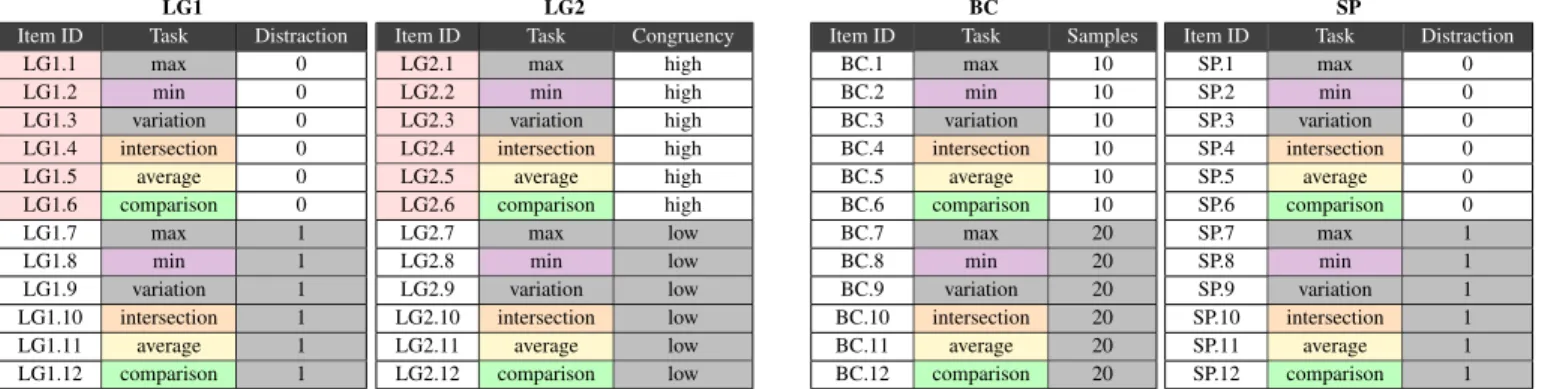
Table 1: Designs of line graph test 1 (LG1), line graph test 2 (LG2), bar chart test (BC), and scatterplot test (SP). Only varying dimensions are shown. Each item is repeated 6 times, beginning with a table condition (repetitions are not shown). Pink cells in the Item ID column indicate duplicate items in tests LG1 and LG2. Tasks with the same color coding are the same. Gray cells in the Distraction, Question Congruency, and Samples columns indicate difference with white cells. The Distraction column uses a binary encoding: 0 = no distractors, 1 = presence of distractors.
planet to settle on. Please help these people determine what the most hospitable planet is by answering the following series of questions as quickly and accurately as possible.
Data We used a dataset with a low-local and medium-global level of variability: the monthly evolution of unemployment in different countries between the years 2000 and 2008. Country names were changed to science-fiction planet names listed in Wikipedia, and years were modified to fit the task scenario.
Priming and Pacing Before each new item, examinees were primed with the upcoming graph type, so that the concepts and op-erations necessary for information extraction could be set up [41]. To separate the time required to read questions and answer them, and to make sure examinees fully comprehended the question/task at hand, a specific pacing was given to each block of repetitions. First, the question was displayed (full page). At the bottom of this was a label “Proceed to graph framework”; this led participants to the table head-ers or graphical framework with appropriate titles and labels. Below was displayed a button labeled “Display data”. When this button was activated, the graph or table was shown and the answer could be given. As mentioned, every block of repetitions began with a condition in which the data were shown in table form. This was preferred so as to remove potential effects caused by the setup of high-level operations for solving a particular kind of problem.
To make sure ability was being tested (and not capacity), we set an 11s timer for each repetition. This was based on the mean time required to answer the items of our pilot studies.
Response format To respond, examinees clicked on one of sev-eral possible answers, displayed in the form of buttons at the bottom of the interface. In some cases, correct answers were not directly dis-played. For example, certain values required for answering were not explicitly shown with labeled ticks on the graph’s axis. This was done to test examinees’ ability to make confident estimations (i. e., to han-dle uncertainty [37]). And although the graphs used color coding to represent the different planets, the buttons did not. This ensured that examinees translated the answer retrieved in the visual domain back into the data domain.
4.1.2 Setup
Participants To our knowledge, no particular number of samples is recommended for IRT modeling. We recruited 40 participants on MTurk. Turkers were required to have a 98% acceptance rate and a to-tal of 1000 or more HITS approved. While the validity of calibrating tests using MTurk may be debated due to lack of control over certain experimental conditions [22], we wanted to perform our calibration with results from a wide variety of people.
Coding 6 Turkers spent less than 1.5 s on average reading and answering item questions; they were considered as random clickers, and their results removed from further analysis. All Turkers for whom results were retained were native English speakers.
The remaining data were sorted according to item and repetition ID (assigned before randomization). Responses for the first repetitions (table conditions) were removed. A score dataset (LG1s) was then created in accord with the requirements of IRT modeling: correct an-swers were scored 1 and incorrect anan-swers 0. Scores for each series of item repetitions (Boolean values) were compressed by taking the mean values and rounding these, resulting in 12 sets of dichotomous item scores for each examinee.
4.1.3 Results
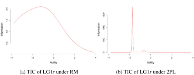
The purpose of the design phase is to remove items that are unhelpful for distinguishing between low and high levels of VL. To do so, we need to: 1) check that the simplest variant of IRT models (i. e., the Rasch model) fits the data, 2) find the best variant of the model to get the most accurate characteristic values for each item, and 3) assess the usefulness of each item with regard to the testing of low ability levels. Checking the Rasch model The Rasch model (RM) was fitted to the score dataset. A 200 sample parametric Bootstrap goodness-of-fit test using Pearson’sχ2statistic revealed a non-significantp-value for LG1s (p > 0.54), suggesting an acceptable fit3. The Test Informa-tion Curve (TIC) is shown in Fig. 1a. It reveals a near-normal distri-bution of test information across different ability levels, with a slight bump around −2, and a peak around −1. This means that the test pro-vides more information about examinees with relatively low abilities (0 being the mean ability level, i. e., that of an average achiever) than about examinees with high abilities.
Finding the right model variant Different IRT models, imple-mented in the ltm R package [43], were fitted to LG1s. A series of pairwise likelihood ratio tests showed that the two-parameter logistic model (2PL) was most suitable.
Assessing the quality of test items Using 2PL, the TIC was plotted again (Fig. 1b). The big spike suggests that several items with difficulty characteristics just above −2 have high discrimination values (a-values). This is confirmed by the very steep Item Charac-teristic Curves (ICCs) (Fig. 3a) of items LG1.1, LG1.4, and LG1.9 (a > 51). This can also explain the distortion in the normal distribu-tion in Fig. 1a.
The probability estimates show that examinees with average abili-ties have a 100% probability of giving a correct answer to the easiest items (LG1.1, LG1.4, and LG1.9), and a 41% probability of giving a
(a) TIC of LG1s under RM (b) TIC of LG1s under 2PL
Fig. 1: Test Information Curves (TICs) of the score dataset of the first line graph test under the original constrained Rasch model (RM) (a) and the two-parameter logistic model (2PL) (b). The ability scale shows theθ-values. The slight bump in the normal distribution of (a) can be explained by the presence of several highly discriminating items, as shown by the big spike in (b).
Fig. 2: Test Information Curve of the score dataset of the second line graph test under the original constrained Rasch model. The test infor-mation is normally distributed.
(a) ICCs of LG1s under 2PL (b) ICCs of LG2s under RM
Fig. 3: Item Characteristic Curves (ICCs) of the score datasets of the first line graph test (LG1s) under the original the two-parameter lo-gistic model (a), and of the second line graph test (LG2s) under the constrained Rasch model (b). The different curve steepnesses in (a) are due to the fact that 2PL computes individual discrimination values for each item, while RM sets all discrimination values to 1.
correct answer to the hardest item (LG1.11). However, LG1.11 has a relatively low discrimination value (a < 0.7), and so may be consid-ered not very useful for distinguishing between ability levels. 4.1.4 Discussion
IRT modeling appears to be a solid approach for our design phase. Our results (Fig. 1) show that LG1 is useful for differentiating between examinees with relatively low abilities, but not so much for ones with high abilities.
The slight bump in the distribution of the TIC (Fig. 1a) suggests that there are several test items that are quite effective for distinguishing between ability levels lower than −2. This is confirmed by the spike in Fig. 1b, indicating the presence of highly discriminating items.
Fig. 3a reveals that several items in the test have identical difficulty and discrimination characteristics. Some of these could therefore be considered for removal, as they only provide redundant information. Similarly, item LG1.11, which has a low discrimination characteristic, could be dropped as it is less efficient than others for differentiating between ability levels.
4.1.5 Line Graphs 2: General Design
Our second line graph test (LG2) also used a low number of varying dimensions, limited to tasks and question congruency. The test used four samples for the stimuli, and a single layout with single scales. The same task scenario, dataset, pacing, and response format were kept, as well as the five repetitions, the initial table condition, and the 11s timer. A summary is given in Table 1. Half of the test’s items were designed to be identical to items in LG1 (displayed in pink in Table 1) to ensure that the results provided by the IRT modeling were consistent.
40 participants were recruited on MTurk; the work of 3 Turkers was rejected, for the same reason as above.
4.1.6 Results and Discussion
Our analysis was driven by the requirements listed above. Data were sorted and encoded in the same way as before, and a score dataset for LG2 was obtained (LG2s).
RM was fitted to the score dataset, and the goodness-of-fit test re-vealed an acceptable fit (p > 0.3). The pairwise likelihood ratio test showed that RM fitted best. Fig. 2 shows that the Test Information Curve is normally distributed, with an information peak roughly cen-tered around −1, indicating that like LG1, this test mostly provides information about examinees with abilities below average.
The Item Characteristic Curves were plotted (Fig. 3b) and com-pared to those of our first test (Fig. 3a) to make sure that the identical items in LG1 and LG2 had similar difficulty distributions. While it cannot be expected that each identical item has the exact same charac-teristics, since item characteristics are relative to individual tests, the order of their difficulty should be consistent. To illustrate this point, consider a simple numeracy test with two items: 10 + 20 (item 1) and 17 + 86 (item 2). It should be assumed that item 1 is easier than item 2. In other words, the difficulty characteristic of item 2 should be higher than that of item 1. Now if we add another item to the test, say 51 × 93 (item 3), the most difficult item in the previous version of the test (item 2) will no longer seem so difficult. However, it should still be more difficult than item 1.
Fig. 3 shows some slight discrepancies in the difficulty of items 1, 3, and 6 between the two tests. However, the fact that item LG1.3 is further to the left in Fig. 3a is misleading. It is due to the characteris-tics of items LG1.1 and LG1.4. These have extremely higha-values. Therefore, while theirb-values are slightly higher than that of LG1.3, the probability of success of an average achiever is higher for these items than it is for LG1.3 (1> 0.94). Furthermore, the difficulty char-acteristics of LG1.3 and LG2.3 are very similar (0.94 ≃ 0.92). Thus the only exception in the ordering of item difficulties is item 6, which is estimated to be more difficult than item 2 in LG1s, and not in LG2s.
We stress that each item characteristic value is not absolute: it is relative to the latent trait that the test is attempting to uncover. Nev-ertheless, the fact that the difficulty of identical items was generally preserved across LG1 and LG2 (with the exception of item 6) sug-gests that these traits may be the same for both tests (i. e., ability to read line graphs). To examine this, we equated the test scores (i. e., we joined them) using a common item equation approach. RM was fitted to the resulting dataset, and the goodness-of-fit test showed an accept-able fit. 2PL provided best fit. Individual item characteristics were generally preserved, with the exception of item 6 which, interestingly, ended up with difficulty and discrimination characteristics very simi-lar to those of item 2. This indicates that the two tests cover the same latent trait. Thus, although item characteristics are slightly adjusted by the equation (e. g., item 6), and therefore this approach should be preferred when possible, it can be assumed that items in LG1 can be transposed to LG2 (and vice-versa) without hindering the overall co-herence of each test.
4.2 Assessment Phase
Having shown that our test items have a sound basis in theory, we now turn to the assessment of examinees’ levels of visualization literacy. To do so, we inspect the ability scores, derived from the fitted IRT models. Essentially, these scores represent examinees’ standings (θ) on the latent trait. They have great predictive power as they can deter-mine the probability of success on items that have not been answered, provided that these items follow the same latent variable scale as other test items that have been answered. Thus, these scores can help predict how well an examinee will perform on a given test. As such, they are perfect indicators for assessing VL.
LG1 revealed 27 different ability levels, ranging from −1.85 to 1. These 27 levels correspond to unique response (score) patterns. While a standard testing method would simply sum up the correct responses, our method considers each response individually, with regard to the difficulty of the item it was given for, before deriving the ability score. The distribution of ability scores for LG1 was nearly normal, with a slight bump around −1.75. 40.7% of participants had ability scores above average (i. e.,θ > 0), and the mean ability was −0.27.
LG2 revealed 33 different ability levels, ranging from −1.83 to 1.19. The distribution was also nearly normal, with a bump around −1. 39.4% of participants had ability scores above average, and the mean ability was −0.17.
These results show that most recruited Turkers had somewhat below average levels of visualization literacy for line graphs. However, the means are close to zero, and the distributions nearly normal. This suggests that most Turkers, while below, are close to average. It is important to point out that, just like item characteristics, ability scores are relative to a latent trait. If ability scores between different tests are to be compared, the latent traits in each must be the same.
Finally, while it should be interesting to develop broader ranges of item complexities for the line graph stimulus (by using the common item equation approach), thus extending the psychometric quality of the tests, we consider LG1 and LG2 to be sufficient for our current line of research. Overall, we believe that these low levels of difficulty reflect the overall simplicity of, and massive exposure to, line graphs.
5 EXTENSIONS
To further test the validity of our method, and to see whether it applies to other types of visualizations, we created two additional tests: one for bar charts (BC) and one for scatterplots (SP). This section presents the design and assessment phases of these tests.
5.1 Design Phase
5.1.1 Bar Charts: General Design
Like LG1 and LG2, the design of our bar chart test (BC) was based on the principles described in Section 3. The varying factors were restricted to tasks and samples; a summary is given in Table 1. The same task scenario was used. The dataset presented life expectancy in various countries, with country names again changed to names of fictitious planets. The 11 s timer was kept.
(a) TIC of BCs under RM (b) ICCs of BCs under RM
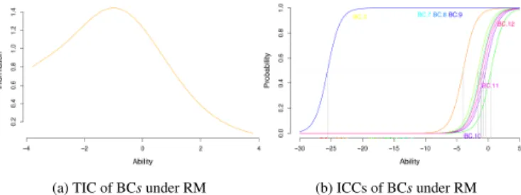
Fig. 4: Test Information Curve (a) and Item Characteristic Curves (b) of the score dataset of the bar chart test under the constrained Rasch model. The TIC in (a) is not normally distributed because of several very low difficulty items, as shown by the curves to the far left of (b).
(a) TIC of the subset of BCs under RM (b) ICCs of the subset of BCs under RM
Fig. 5: Test Information Curve (a) and Item Characteristic Curves (b) of the subset of the score dataset of the bar chart test under the con-strained Rasch model. The subset was obtained by removing the very low difficulty items shown in Fig. 4b.
The only difference with the factors used in the previous tests (apart from the stimulus) was the variation task, as this was more of a trend detection task in the line graph tests. Bar charts are sub-optimal for determining trends, so the task was replaced by “global similarity de-tection”, as done in [23] (e. g., “Do all the bars have the same value?”). 40 participants were recruited on MTurk. The work of 6 Turkers was rejected, for the same reason as mentioned above.
5.1.2 Results and Discussion
Our analysis was driven by the same requirements as the ones set for the line graph tests. Data were sorted and encoded in the same way as before, resulting in a score dataset for BC (BCs).
RM was fitted to the data; the goodness-of-fit test revealed an ac-ceptable fit (p > 0.37), and the pairwise likelihood ratio tests proved that RM fit best. Fig. 4a shows that the Test Information Curve is not normally distributed. This is due to the presence of several ex-tremely low difficulty (i. e., easy) items (BC.3, BC.7, BC.8, and BC.9; b = −25.6), as shown in Fig. 4b. Inspecting the raw scores for these items revealed a 100% success rate. Thus, they were considered too easy for the assessment we wished to make and were removed. Simi-larly, items BC.1 and BC.2 (for both,b < −4) were also removed.
To check the coherence of the subset test, RM was fitted again to the new set of scores. Goodness-of-fit was maintained (p > 0.33), and RM still fitted best. The new TIC (Fig. 5a) is normally distributed, and shows that this subset test mainly provides information for low ability levels, with a peak aroundθ ≃ −1, meaning that like LG1 and LG2, the subset of BC is useful for differentiating examinees with relatively low abilities from ones with average abilities. Only one item (BC.5, see Fig. 5b) is above average difficulty.
5.1.3 Scatterplots: General Design
For our scatterplot test (SP), all design attributes of the previous tests were once again used. The varying factors were tasks and distraction, as shown in Table 1. Slight changes were made to some of the tasks since scatterplots use two spatial dimensions (as opposed to bar charts and line graphs). For example, stimuli with distractors in LG1 only required examinees to focus on one of several samples; here, stimuli
(a) TIC of SPs under 2PL (b) ICCs of SPs under 2PL
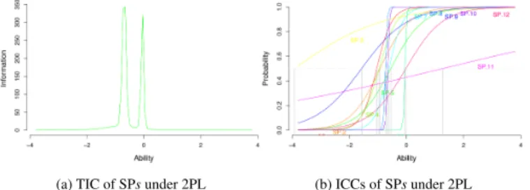
Fig. 6: Test Information Curve (a) and Item Characteristic Curves (b) of the score dataset of the scatterplot test under the two-parameter lo-gistic model. The TIC (a) shows that there are several highly dis-criminating items, which is confirmed by the very steep curves in (b). In addition, (b) shows that there are also a two poorly discriminating items, represented by the very gradual slopes of items SP.3 and SP.11.
(a) TIC of the subset of SPs under 2PL (b) ICCs of the subset of SPs under 2PL
Fig. 7: Test Information Curve (a) and Item Characteristic Curves (b) of the subset of the score dataset of the scatterplot test under the two-parameter logistic model. The subset was obtained by removing the poorly discriminating items shown in Fig. 6b.
with distractors could either require examinees to focus on a single datapoint or on a single dimension. A percentage of adult literacy by expenditure per student in primary school dataset was used.
We had expected that SP might be slightly more difficult and items would therefore require more time to complete. However, a pilot test on 10 Turkers showed the average response time per item was once again roughly 11 s. Therefore the 11 s timer was kept.
40 participants were recruited on MTurk. The work of 1 Turker could not be kept due to technical (logging) issues.
5.1.4 Results and Discussion
Our analysis was once again driven by the same requirements as be-fore. The same sorting and coding was applied to the data, resulting in the score dataset SPs. The same fitting procedure was then applied, revealing a good fit for RM (p = 0.6), and a best fit for 2PL.
The Test Information Curve (Fig. 6a) shows the presence of several highly discriminating items aroundθ ≃ −1 and θ ≃ 0. The Item Char-acteristic Curves (Fig. 6b) confirm that there are three (SP.6, SP.8, and SP.10; a > 31). However, they also show that two items (SP.3, and SP.11) have quite low discrimination values (a < 0.6).
Here, we set a threshold fora > 0.8. Items SP.3 and SP.11 were thus removed. The resulting subset of 10 items’ scores was fitted once again. RM fitted well (p = 0.69), and 2PL fitted best. The different curves of the subset are plotted in Fig. 7. They show a good amount of information for abilities that are slightly below average (Fig. 7a), which indicates that the subset of SP is also more adequate for testing examinees with relatively low abilities.
5.2 Assessment phase
Here again, we inspected the Turkers’ ability scores. Only the items retained during the analysis were used.
BC revealed 21 different ability levels, ranging from −1.75 to 0.99. The distribution of ability scores was nearly normal, with a slight bump around −1.5. The mean ability was −0.39. However, only 14.3% of participants had ability scores above average.
SP revealed 23 different ability levels, ranging from −1.72 to 0.72. The distribution here was not normal. 43.5% of participants had ability scores above average, and the median ability was -0.14.
These results show that the majority of recruited Turkers had some-what below average levels of visualization literacy for bar charts and scatterplots. The very low percentage of Turkers above average in BC led us to reconsider the removal of items BC.1 and BC.2, as they were not truly problematic. After reintegrating them in the test scores, 21 ability levels were observed, ranging from −1.67 to 0.99, and 42.8% of participants had ability scores above average. This seemed more convincing. However, this important difference illustrates once again the relativity of these values, and shows how important it is to properly calibrate the tests during the design phase.
Finally, we did not attempt to equate these tests, since we ran them independently without any overlapping items (unlike LG1 and LG2). To have a fully comprehensive test, i. e., a generic test for visualization literacy, whatever the type of chart or graph, intermediate tests are re-quired where the stimulus itself is a varying factor. If such tests prove to be coherent (i. e., if IRT models fit the results), then it should be possible to assert that VL is a general trait that allows one to under-stand any kind of graphical representation. Although we believe that the ability to extract information from a visualization varies with ex-posure and habit of use, a study to confirm this is outside of the scope of this paper.
6 FAST, EFFECTIVETESTING
If these tests are to be used as practical ways of assessing VL, the process must be sped up, both in the administration of the tests and in the analysis of the results. While IRT provides essential information on the quality of tests and on the ability of those who take them, it is quite costly, both in time and in computation. This must be changed.
In this section, we present a way in which the tests we have devel-oped in the previous sections can be optimized for future use.
6.1 Test Administration Time
As we have seen, several items can be removed from the tests, while keeping good psychometric quality. However, this should be done carefully, as some of these items may provide useful information (like in the case of BC.1 and BC.2, Sect. 5.2).
We first removed LG1.11 from LG1, as its discrimination value was < 0.8 (see Sect. 5.1.4). We then inspected items with identical diffi-culty and discrimination characteristics, which are represented by the overlapping curves in the ICCs (see Fig. 3). Such items were consid-ered prime candidates for removal, since probability of success can be inferred from the ability scores. There was one group of overlap-ping items in LG1 ([LG1.1, LG1.4, LG1.9]), and two in LG2 ([LG2.1, LG2.3], [LG2.2, LG2.7]). For each group, we kept only one item. Thus LG1.1, LG1.4, LG2.3, and LG2.7 were dropped.
We were forced to reintegrate items BC.1 and BC.2 to BC, as they proved to have a big impact on ability scores (Sect. 5.2). The subset of SP created for the analysis was kept, and no extra items were removed. RM was fitted once again to the newly created subsets of LG1, LG2, and BC; the goodness-of-fit test showed acceptable fits for all (p > 0.69 for LG1, andp > 0.3 for both LG2 and BC). 2PL fitted best for LG1, and RM fitted best for LG2 and BC.
A post-hoc analysis was conducted for each test to see whether the number of repetitions could be reduced (first to three, then to one). Re-sults showed that RM fitted all score datasets using three repetitions. However, several examinees had lower scores. In addition, while BC and SP showed similar amounts of information for the same ability levels, the three very easy items in BC (i. e., BC.3, BC.7, BC.8, and BC.9) were no longer problematic. This suggests that several par-ticipants did not get a score of 1 for these items, and confirms that, for some examinees, more repetitions are needed. Results for one-repetition-tests showed that RM no longer fitted the scores of BC, sug-gesting that first repetitions (with the graph/chart stimulus) are noisy. Therefore, at this point, we decided to keep the five repetitions.
In the end, the redesign of LG1 contained 9 items (with a ≃ 10 min completion time), the redesigns of LG2 and SP contained 10 items (11
min), and the redesign of BC contained 8 items (≃ 9 min).
6.2 Analysis Time and Computational Power
To speed up the analysis, we first considered setting up the procedure we had used in R on a server. However, this solution would have required a lot of computational power, so we dropped it.
Instead, we chose to tabulate all possible ability scores for each test, based on all possible response patterns. An interesting feature of IRT modeling is that it accepts unobserved response patterns (i. e., patterns that do not exist in the empirical data), and partial response patterns (i. e., patterns with missing values). Consequently, we generated every possible pattern for each test. There are 2ni− 1 possibilities for a test
containingniitems. Thus 511 patterns were created for LG1, 1023
for both LG2 and SP, and 255 for BC. We then derived the different ability scores that could be obtained in each test.
To make sure that shortening the tests (i. e., removing certain items) did not greatly affect the ability scores, we derived all ability scores for the full LG1 and LG2 tests. We found some small differences, spe-cially in the upper and lower bounds of ability, but we consider these to be negligible, since our tests were not designed for fine distinction between very low abilities or high abilities. We also tested the im-pact of refitting the models, once the items were removed. For this, we repeated the procedure, using the full LG1 and LG2 tests, but we replaced the Boolean response values for the items considered for re-moval by not available (NA) values. The derived scores were exactly the same as the ones derived from our already shortened (and refitted) tests, which proves that they can be trusted.
Finally, we integrated these ability scores and their correspond-ing response patterns into the web-based, shortened versions of the tests. This way, the scores are immediately available. Consider-ing our original motivation, by administerConsider-ing these online tests, re-searchers can have direct access to participants’ levels of visualiza-tion literacy. Informed decisions can then be made as whether to keep participants for further studies or not. All four tests are ac-cessible at http://peopleviz.gforge.inria.fr/trunk/ vLiteracy/home/
7 METHODOLOGYGUIDELINES
As the preceding sections have shown, we have developed and vali-dated a fast and effective method for assessing visualization literacy. This section summarizes the major steps of our method. It is written in the form of easy “take-away” guidelines.
7.1 Original Design
1. Pay careful attention to the design of all 3 components of a test item, i. e., stimulus, task, and question. Each of these can influence item difficulty, and too much variation may fail to pro-duce a good test (as was seen in our pilot studies).
2. Repeat each item several times. We did 5 repetitions + 1 “ques-tion comprehension” condi“ques-tion for each item. This is important as repeated trials provide more robust measures. Ultimately, it may be feasible to reduce the number of repetitions to 3.4 3. Use a different, and ideally, non-graphical, representation
for the question comprehension condition. We chose a table condition. While our present analysis did not focus on proving its essentialness, we believe that this attribute is important. 4. Randomize order of items and of repetitions. This is common
practice in experiment design, having the benefit of preventing carryover effects.
5. Once the results are in, sort the data according to item and repetition ID, and remove the data for the initial repetitions. 6. Encode examinees’ scores in a dichotomous way, i. e., 1 for
correct answers and 0 for incorrect answers.
7. Calculate the mean score for all repetitions of an item and round the result. This will give a finer estimate of the
exami-4The number of repetitions should be odd, so as to not end up with a mean
score of 0.5 for an item.
nee’s ability since it erases one-time errors which may be due to lack of attention or to clicking on the wrong answer by mistake. 8. Fit the original constrained version of the Rasch model to the data. RM is the simplest variant of IRT models. If it does not fit the data, other variants will not either.
9. Check the fit of the model. Here we used a 200 sample para-metric Bootstrap goodness-of-fit test using Pearsonsχ2statistic. To reveal an acceptable fit, the returnedp-value should not be statistically significant (p > 0.05). In some cases (like in our pi-lot studies), the model may not fit. Option here are to inspect the χ2p-values for pairwise associations, or the two- and three-way
χ2residuals, to find potentially problematic items5.
10. Determine which IRT model variant best fits the data. To test this, series of pairwise likelihood ratio tests can be used. If several models fit, it boils down to how precise the examinee and item characteristics need to be. Generally speaking, it is better to go with the model that fits best. Our experience showed that such models were most often RM and 2PL.
11. Identify potentially useless items. In our examples of LG1 and SP, certain items had very low discrimination characteris-tics. These are not very efficient for differentiating ability levels. They can be removed. In cases like the one for BC, items may also simply be too easy. These items can also be removed, but special care must be taken with regard to the impact on ability scores. Finally, it is important the model be refitted at this stage, (reproducing steps 8 through 10) as removing these items may affect examinee and item characteristics.
7.2 Final Design
12. Identify potentially overlapping items and remove them. If the goal is to design a short test, such items can safely be re-moved, as seen in Sect. 6.1. IRT models should then be refitted to the subsets of item scores, repeating steps 8 through 10. 13. Generate all 2ni
− 1 possible score patterns, where niis the
number of (retained) items in the test. These patterns are series of possible Boolean responses to the test items.
14. Derive the ability scores from the model, using the patterns of responses generated in step 13. These scores represent the range of visualization literacy levels that the test can assess.
15. Integrate the ability scores into the test to make fast, effective, and scalable estimates of people’s visualization literacy.
8 CONCLUSIONS ANDFUTUREWORK
In this paper, we have presented a method based on Item Response Theory for assessing visualization literacy, through the design and evaluation of a series of tests that each cover different aspects of vi-sualization literacy. Our original motivation was to make a series of fast, effective, and reliable tests which researchers could use to detect participants with low VL levels using online studies. In addition, we have proposed a way in which these tests can be redesigned and im-plemented in order to get immediate estimates of examinee’s levels of visualization literacy.
We intend to continue developing these tests, as well as examine their suitability for other kinds of representation (e. g., parallel coor-dinates, node link diagrams, starplots, etc.), and possibly for other purposes. In other contexts like that of a classroom evaluation, tests could be made longer, and broader assessments of visualization liter-acy could be made. This would imply further exploration of the design parameters we have proposed in section 3. Evaluating these parame-ters to find their impact on item difficulty should also be interesting.
Finally, we acknowledge that this work is but a small step into the realm of visualization literacy, which is why we have made our tests available on GitHub for versioning [1]. Ultimately, we hope that this will serve as a foundation for further research into VL.
REFERENCES
[1] https://github.com/INRIA/Visualization-Literacy-101.