Knowledge base curation using constraints

(1)

HAL Id: tel-03102638

https://tel.archives-ouvertes.fr/tel-03102638

Submitted on 7 Jan 2021

HAL is a multi-disciplinary open access archive for the deposit and dissemination of sci-entific research documents, whether they are pub-lished or not. The documents may come from teaching and research institutions in France or

L’archive ouverte pluridisciplinaire HAL, est destinée au dépôt et à la diffusion de documents scientifiques de niveau recherche, publiés ou non, émanant des établissements d’enseignement et de recherche français ou étrangers, des laboratoires

Knowledge base curation using constraints

Thomas Pellissier-Tanon

To cite this version:

Thomas Pellissier-Tanon. Knowledge base curation using constraints. Databases [cs.DB]. Institut Polytechnique de Paris, 2020. English. �NNT : 2020IPPAT025�. �tel-03102638�

(2)

NNT

:

2020IPP

A

T025

Knowledge Base Curation

using Constraints

Thèse de doctorat de l’Institut Polytechnique de Paris préparée à Télécom Paris École doctorale n◦₆₂₆

École doctorale de l’Institut Polytechnique de Paris (ED IP Paris)

Spécialité de doctorat: Informatique

Thèse présentée et soutenue à Palaiseau, le 7 septembre 2020, par

T

HOMAS

P

ELLISSIER

T

ANON

Composition du Jury :

Serge Abiteboul

Directeur de recherche émérite, INRIA (DI ENS) Examinateur Antoine Amarilli

Maître de conférence, Télécom Paris Co-encadrant de thèse

Laure Berti-Equille

Directeur de recherche, IRD Présidente et Rapporteure

Markus Krötzsch

Professeur, TU Dresden Rapporteur

Nathalie Pernelle

Professeur, Université Sorbonne Paris Nord Examinatrice Simon Razniewski

Senior researcher, Max Planck Institute for Informatics Examinateur Fabian Suchanek

Professeur, Télécom Paris Directeur de thèse

Danai Symeonidou

(3)

(4)

Knowledge Base Curation using Constraints

Thomas Pellissier Tanon

September 7th, 2020

(5)

(6)

Abstract

Knowledge bases are huge collections of primarily encyclopedic facts. They are widely used in entity recognition, structured search, question answering, and other tasks. These knowledge bases have to be curated, and this is a crucial but costly task. In this thesis, we are concerned with curating knowledge bases automatically using constraints.

Our first contribution aims at discovering constraints automatically. We improve standard rule mining approaches by using (in-)completeness meta-information. We show that this information can increase the quality of the learned rules significantly.

Our second contribution is the creation of a knowledge base, YAGO 4, where we statically enforce a set of constraints by removing the facts that do not comply with them.

Our last contribution is a method to correct constraint violations automatically. Our method uses the edit history of the knowledge base to see how users corrected violations in the past, in order to propose corrections for the present.

(7)

(8)

Remerciements

Tout d’abord, j’aimerais remercier mes directeurs de thèse Fabian Suchanek et Antoine Amarilli pour leur soutien durant ces trois années de thèse. Ce travail n’aurait pas été possible sans eux. Merci beaucoup pour m’avoir laissé choisir et conduire les directions dans lesquelles mener les travaux présentés dans cette thèse, tout en vous rendant très disponibles pour m’aider et me guider.

Merci tout spécialement à Fabian pour avoir relu et réécrit bon nombre de mes articles en supportant avec une patience admirable mes bien trop nombreuses fautes d’anglais.

Merci à mes rapporteurs, Laure Berti-Equille et Markus Krötzsch pour le temps passé à relire cette thèse. Merci à tous les membres de mon jury pour avoir accepté d’y participer.

Merci à toutes les personnes avec qui j’ai collaboré sur les travaux présentés dans cette thèse. Tout spécialement à Gerhard Weikum et Daria Stepanova qui m’ont accueilli pour un stage au Max Planck Institute for Informatics. Sans oublier Camille Bourgaux dont l’aide m’a été très précieuse. Mais aussi un grand merci à Simon Razniewski, Paramita Mirza Thomas Rebele et Lucie-Aimée Kaffee avec qui j’ai eu le plus grand plaisir à collaborer.

Merci aussi à Denny Vrandečić, Serge Abiteboul, Eddy Caron, Pierre Senellart et David Montoya pour m’avoir encadré avant cette thèse et permis de mûrir ce projet.

Merci aux membres de l’équipe DIG pour les bons moments passés ensemble. Entre autres, à Albert, Armand, Arnaud, Camille, Etienne, Favia, Jacob, Jean-Benoît, Jean-Louis, Jonathan, Julien, Julien, Louis, Marc, Marie, Maroua, Mauro, Mikaël, Miy-oung, Mostafa, Nathan, Ned, Oana, Pierre-Alexandre, Quentin, Tho-mas, Thomas et Ziad.

Merci enfin à ma famille pour tout le soutien qu’elle m’a donné durant ces trois années. Merci surtout à Mélissa pour son soutien sans faille malgré les trop nombreuses heures décalées passées à travailler.

(9)

(10)

Chapter 1 Introduction

1.1 Motivation

Knowledge bases (KBs) are sets of machine-readable facts. They contain entities and relations about them. For example an encyclopedic knowledge base could contain entities about people like Jean-François Champollion or places like Paris, and named relations like livedIn(Jean-François_Champollion, Paris) to state that Jean-François Champollion lived in Paris. Well-known knowledge bases in this area include Wikidata (Vrandecic and Krötzsch, 2014), YAGO (Suchanek, Kasneci, and Weikum, 2007), Freebase (Bollacker et al., 2008), DBpedia (Bizer et al., 2009) or the Google Knowledge Graph. Such knowledge bases are used to display fact sheets like in Wikipedia or in the Google and Bing search engines. They are also used to directly answers user questions like in Alexa or Siri. But knowledge bases are also used for other kinds of contents and use cases. For example, Amazon and eBay maintain knowledge bases of the products they sell and Uber maintains a food knowledge base to help its customers choose a restaurant.

Some knowledge bases are very large. For example, Wikidata contains 81M entities1 and Freebase 39M. Some of these projects use software pipelines to build the knowledge base automatically from one or multiple existing sources. For ex-ample, DBpedia is built by a set of extractors from Wikipedia content. Others are using a crowd of contributors, paid or volunteer, to fill the knowledge base. This is the case of Wikidata, which has more than 40k different editors per month.

As a consequence, knowledge bases often exhibit quality problems, originating from edge cases in the conversion pipelines, good-faith mistakes, or vandalism in the crowd-sourced content. For example Zaveri, Kontokostas, et al., 2013 found that 12% of the DBpedia triples have some kind of issue. Even crowd-sourced knowledge bases often rely significantly on automated importation or curation

(15)

pipelines. 43% of Wikidata edits in March 2020 have been done using automated tools.

To fight such problems, many knowledge bases contain a constraint system. One of the most basic kinds of constraint is stating that the values of a given property should have a given type. For example, a knowledge base could enforce that the values of the birthPlace property should be strings representing a date. Constraints can also be more complex stating e.g., that a person can have at most 2 parents (cardinality restrictions) or that an entity cannot be a person and a place at the same time (disjunctions). Some of these constraints are enforced by the knowledge base. For example, the OWL formalism itself requires that properties whose values are literals (string, dates...) have to be disjoint from the ones whose values are entities. However, these constraints are often violated in practice. For example, as of March 20th, 2020, Wikidata has 1M “domain” constraint violations and 4.4M “single value” constraint violations. Thus, there is a need for tools to filter out such problems from the knowledge base. There is also a need for tools that help the knowledge base curators repair these violations in an automated or semi-automated way.

This thesis provides some new approaches and techniques to improve the state on the art on this complex task.

1.2 Presented Contributions

The first chapter of this thesis, Chapter 2, presents general preliminaries on knowl-edge bases and rule mining. The main work is composed of 3 parts.

Part I, presents improvements to the rule mining problem. More precisely, Chapter 3 presents a novel approach that improves rules mining over incomplete knowledge bases by making use of cardinality information. This allows mining rules of higher quality. These can then be used in order to complete the knowl-edge base or as constraints to flag problems in the data. Our approach works by introducing a new rule quality estimation measure, the completeness confidence. The completeness confidence takes into account the number of expected objects for given subjects and predicates to better assess the quality of the rules. We show that this measure does not require cardinality information on all the knowl-edge base entities to be effective. We evaluated this completeness confidence both on real-world and synthetic datasets, showing that it outperforms existing mea-sures both with respect to the quality of the mined rules and the predictions they produce.

Chapter 4 presents an approach to increase the number of available cardinality metadata, especially to improve the quality of the rules mined using the complete-ness confidence.

(16)

The content of these two chapters was published at ISWC 2017 where it was nominated for the best student paper award. An invited short version of the paper has been presented at IJCAI 2018:

Thomas Pellissier Tanon, Daria Stepanova, Simon Razniewski, Paramita Mirza, and Gerhard Weikum. “Completeness-Aware Rule Learning from Knowledge Graphs”. Full paper at ISWC 2017. https://doi.org/10. 1007/978-3-319-68288-4_30

Thomas Pellissier Tanon, Daria Stepanova, Simon Razniewski, Paramita Mirza, and Gerhard Weikum. “Completeness-aware Rule Learning from Knowledge Graphs”. Invited paper at IJCAI 2018. https://doi.org/ 10.24963/ijcai.2018/749

Part II of this thesis presents an approach of static constraint enforcement. More precisely, it presents YAGO 4, a knowledge base is basically a simpler and cleaner version of Wikidata. We built this knowledge base using a declarative mapping and constraint enforcement pipeline. YAGO 4 can be seen as an example of a knowledge base that ensures quality by filtering out constraint violations. This work has been published as a resource paper at ESWC 2020:

Thomas Pellissier Tanon, Gerhard Weikum, and Fabian M. Suchanek. “YAGO 4: A Reason-able Knowledge Base”. Resource paper at ESWC 2020. https://doi.org/10.1007/978-3-030-49461-2_34

Part III presents contributions to the task of dynamically learning how to enforce constraints. Chapter 6 discusses a novel problem: learning how to fix constraint violations using the edit history of a knowledge base. We present a for-malism of the problem and an algorithm to extract “past corrections” of constraint violations from the knowledge base history. To solve this problem, the chapter suggests two different approaches: one based on rule mining and the other one using neural networks, the latter providing better accuracy but no explanation of its predictions. We validated both approaches experimentally on Wikidata, show-ing substantial improvements over baselines. This work has been presented at TheWebConf 2019. The neural network approach is currently under review:

Thomas Pellissier Tanon, Camille Bourgaux, and Fabian M. Suchanek. “Learning How to Correct a Knowledge Base from the Edit History”. Full paper at WWW 2019. https://doi.org/10.1145/3308558.3313584

(17)

Thomas Pellissier Tanon and Fabian M. Suchanek. “Neural Knowledge Base Repairs”. Under review at ISWC 2020.

Chapter 7 is an annex of the previous chapter. It presents a system we imple-mented to query the edit history of Wikidata efficiently. It was used to extract the data used to evaluate the approaches presented in the previous chapter. This work has been demoed at ESWC 2019:

Thomas Pellissier Tanon and Fabian M. Suchanek. “Querying the Edit History of Wikidata”. Demo at ESWC 2019. https://doi.org/10. 1007/978-3-030-32327-1_32

1.3 Other works

During my Ph.D., I contributed to some other works that are not presented in this thesis.

I presented my master thesis at the Linked Data on The Web workshop. This work was done with David Montoya under the supervision of Serge Abiteboul, Pierre Senellart, and Fabian M. Suchanek. The master thesis was about building a knowledge integration platform for personal information. This system is able to synchronize in both directions from datasources such as emails, calendars, and contact books. It also aligns and enriches the data. This work was also demoed at CIKM:

David Montoya, Thomas Pellissier Tanon, Serge Abiteboul, Pierre Senel-lart, and Fabian M. Suchanek. “A Knowledge Base for Personal Infor-mation Management”. Paper at the LDOW workshop collocated with WWW 2018. http://ceur-ws.org/Vol-2073/article-02.pdf

David Montoya, Thomas Pellissier Tanon, Serge Abiteboul, and Fabian M.Suchanek. “Thymeflow, A Personal Knowledge Base with Spatio-temporal Data”. Demo at CIKM 2016. https://doi.org/10.1145/ 2983323.2983337

I also published an earlier work on using grammatical dependencies for question answering over knowledge bases. This work was demoed at ESWC and the dataset to train such systems has been presented as a poster at ISWC:

(18)

Thomas Pellissier Tanon, Marcos Dias de Assunção, Eddy Caron, and Fabian M. Suchanek. “Demoing Platypus - A Multilingual Question Answering Platform for Wikidata”. Demo at ESWC 2018. https: //doi.org/10.1007/978-3-319-98192-5_21

Dennis Diefenbach, Thomas Pellissier Tanon, Kamal Deep Singh, and Pierre Maret. “Question Answering Benchmarks for Wikidata”. Poster at ISWC 2017. http://ceur-ws.org/Vol-1963/paper555.pdf

Furthermore, together with Lucie-Aimée Kaffee, we conducted a study of the stability of the Wikidata schema. We analyzed the stability of the data based on the changes in the labels of properties in six languages. We found that the schema is overall stable, making it a reliable resource for external usage. This work was presented at the WikiWorshop:

Thomas Pellissier Tanon and Lucie-Aimée Kaffee. “Property Label Stabil-ity in Wikidata: Evolution and Convergence of Schemas in Collaborative Knowledge Bases”. Short paper at the WikiWorkshop collocated with WWW 2018. https://doi.org/10.1145/3184558.3191643

I also helped a Ph.D. student in the team, Thomas Rebele, on his work on evaluating Datalog using Bash shell commands. I formalized the problem and provided a converter between Datalog and relational algebra. Our method allows preprocessing large tabular data in Datalog — without indexing the data. The Datalog query is translated to Unix Bash and can be executed in a shell. Our experiments have shown that, for the use case of data preprocessing, our approach is competitive with state-of-the-art systems in terms of scalability and speed, while at the same time requiring only a Bash shell on a Unix system. This work has been published at ISWC:

Thomas Rebele, Thomas Pellissier Tanon, and Fabian M. Suchanek. “Bash Datalog: Answering Datalog Queries with Unix Shell Com-mands”. Full paper at ISWC 2018. https://doi.org/10.1007/ 978-3-030-00671-6_33

(19)

(20)

Chapter 2 Preliminaries

2.1 Knowledge bases

A knowledge base (KB) is an interlinked collection of factual information. A knowledge base can be represented as a graph. Nodes represent entities (like the human Elvis Presley, or the notion of a human) and directed labeled edges represent facts about these entities. For example, an edge labeled “type” from the node representing Elvis Presley to the node representing the notion of a human encodes that Elvis Presley is a human. See Figure 2.1 for a graphical example of a knowledge base. In this work, we use description logics (DL) (Baader et al., 2003) as a knowledge base language, and more specifically the ones that fall under the OWL 2 DL formalism (Motik, Patel-Schneider, and Grau, 2012).

Syntax

We assume a set NC of concept names (unary predicates, also called classes), a

set NR of role names (binary predicates, also called properties), and a set NI of

individuals (also called constants).

Definition 2.1 (ABox). An ABox (dataset) is a set of concept assertions and role assertions which are respectively of the form A(a) or R(a, b), where A ∈ NC,

R ∈ NR, and a, b ∈ NI.

Definition 2.2 (TBox). A TBox (ontology) is a set of axioms that expresses relationships between concepts and roles. (e.g., concept or role hierarchies, role domains and ranges...). Their form depends on the description logic L in question. We only consider here description logics L that fall under the OWL 2 DL formalism (Motik, Patel-Schneider, and Grau, 2012).

(21)

Some commonly found building blocks in description logics formulas are the fol-lowing:1

• > is the most general concept containing all individuals. • ⊥ is the empty concept.

• {a1, . . . , an} is the concept containing only the individuals a1, . . . , an.

• ¬A is the complement of the concept A (i.e., all individuals not in A). • A t B is the concept that contains all individuals in A or B.

• A u B is the concept that contains all individuals that are in both A and B. • ∃R · B is the concept containing all a such that there exists b with R(a, b)

and B(b).

• R− _{is the inverse role of R i.e., informally, R(a, b) if, and only if, R}−_{(b, a).}

This notation can be used to create axioms like the following:

• A v B states that all individuals in the concept A are also in the concept B. • A ≡ B states that A and B are equivalent i.e., A v B and B v A.

• P v R states that all facts of a role P are also in a role R.

• P ≡ R states that P and R are equivalent i.e., P v R and R v P .

• (func R) states that R if functional i.e., informally, for all a, b1 and b2 if

R(a, b1) and R(a, b2) then b1 = b2.

• (trans R) states that R if transitive i.e., informally, for all a, b and c if R(a, b) and R(b, c) then R(a, c).

Definition 2.3 (Knowledge base). A knowledge base K = (T , A) is a pair of a TBox T and an ABox A.

The knowledge base can also be written as a set of RDF triples (Cyganiak et al., 2014) hs, p, oi where s is the subject, p is the property, and o the object. A concept assertion A(a) is written as ha, rdf:type, Ai, and a role assertion R(a, b) as ha, R, bi. The TBox can also be written with RDF triples using the mapping defined in Motik and Patel-Schneider, 2012.

1_{For brevity we do not recall all OWL 2 DL formulas and axiom elements. They are all}

(22)

Zeus Chronos Rhea male female hasParent hasChild hasGender hasGender hasGender

Figure 2.1 – Example knowledge base

Example 2.4. Here is an example of knowledge base about Greek gods:

T = { ∃hasParent v Human, ∃hasChild v Human, ∃hasGender v Human, hasParent−≡ hasChild , ∃hasGender−v {male, female} }

A = { hasGender (Zeus, male), hasGender (Cronos, male), hasGender (Rhea, female), hasParent (Zeus, Chronos), hasChild (Rhea, Zeus), }

The TBox states that if you have a parent, a child, or a gender then you are a human, that hasChild is the inverse property of hasParent, and that the two possible values for the hasGender relation are male and female. The ABox is represented graphically in Figure 2.1.

The ABox and the TBox entail the following facts: Human(Zeus), Hu-man(Chronos), Human(Rhea), hasParent (Zeus, Rhea) and hasChild (Chronos, Zeus).

Semantics

We recall the standard semantics of description logic knowledge bases (Baader et al., 2003).

Definition 2.5 (Interpretation). An interpretation has the form I = (∆I, ·I), where ∆I is a non-empty set and ·I is a function that maps each a ∈ NI to

aI ∈ ∆I_{, each A ∈ N}

C to AI ⊆ ∆I, and each R ∈ NR to RI ⊆ ∆I× ∆I.

The function ·I is straightforwardly extended to general concepts and roles. For example:2

• >I _{= ∆}I

• ⊥I _{= ∅}

(23)

• {a1, . . . , an}I = {aI1, . . . , a I n} • (¬A)I _{= ∆}I _{\ A}I • (A t B)I _{= A}I _{∪ B}I • (A u B)I _{= A}I _{∩ B}I • (∃R · B)I _{= {a | ∃b (a, b) ∈ R}I_{, b ∈ B}I_} • (R−₎I _{= {(b, a) | (a, b) ∈ R}I_} An interpretation I satisfies:3 • A(a) if aI _{∈ A}I • R(a, b) if (aI_{, b}I_{) ∈ R}I • A v B, if AI _{⊆ B}I • P v R, if PI _{⊆ R}I

• (func R) if ∀a, b1, b2 ∈ ∆I (a, b1) ∈ RI ∧ (a, b2) ∈ RI =⇒ b1 = b2

• (trans R) if ∀a, b, c ∈ ∆I _{(a, b) ∈ R}I _{∧ (b, c) ∈ R}I _{=⇒ (a, c) ∈ R}I

We write I |=L α if I satisfies the description logic axiom α according to the

description logic used L.

Definition 2.6 (Model). An interpretation I is a model of K = (T , A) if I satisfies all axioms in T and all assertions in A according to L.

Definition 2.7 (Consistency). A knowledge base is consistent if it has a model. Definition 2.8 (Entailment). A knowledge base K entails a description logic axiom α in L if I |=Lα for every model I of K. We write K |=Lα in this case.

Definition 2.9 (Unique name assumption). The unique name assumption re-stricts the set of possible interpretations I = (∆I, ·I) of K to only the ones where ·I _{is injective on individuals. It means that each individual a ∈ N}

I has a different

interpretation i.e., each real world entity is represented by at most one individual. 3_{See Motik, Patel-Schneider, and Grau, 2012 for the semantic of all OWL 2 DL axioms.}

(24)

Ideal knowledge base

Following Darari, Nutt, et al., 2013, we define the the ideal knowledge base Ki_,

which contains all correct facts over NC, NR and NI that hold in the real world.

Of course, Ki _{is an imaginary construct whose content is generally not known.}

We will present a method that can deduce instead to which extent the available knowledge base approximates/lacks information compared to the ideal knowledge base, as in “Einstein is missing 2 children and Feynman none”.

2.2 Queries

The description logic formalism explained in the previous section allows us to do entailments on the knowledge base. However, answering queries like “who are the people who died where they were born” is not possible with the description logic formalism we described. This is why we now introduce some variations of the concept of queries.

Conjunctive and disjunctive queries

Definition 2.10 (Conjunctive query). A conjunctive query takes the form q(~x) = ∃~y ψ(~x, ~y), where ψ is a conjunction of atoms of the form A(t) or R(t, t0) or of equalities t = t0, where t, t0 are individual names from NI or variables from ~x ∪ ~y,

A ∈ NC, and R ∈ NR .

Example 2.11. The query q(x) = Person(x) ∧ birthPlace(x, Paris) returns all the people born in Paris.

The query q0(x) = ∃y Person(x) ∧ birthPlace(x, y) ∧ deathPlace(x, y) returns all the people who died where they were born.

If ~x = ∅, q is a boolean conjunctive query. A boolean conjunctive query q is satisfied by an interpretation I, written I |= q, if there is a homomorphism π mapping the variables and individual names of q into ∆I such that: π(a) = aI for every a ∈ NI,

π(t) ∈ AI for every concept atom A(t) in ψ, (π(t), π(t0)) ∈ RI for every role atom R(t, t0) in ψ, and π(t) = π(t0) for every t = t0 in ψ. We also consider as boolean conjunctive queries the queries true and false which are respectively always and never satisfied by an interpretation. A boolean conjunctive query q is entailed by a knowledge base K, written K |= q, if, and only if, q is satisfied by every model of K.

A tuple of constants ~a is a (certain) answer to a conjunctive query q(~x) on a knowledge base K if K |= q(~a) where q(~a) is the boolean conjunctive query obtained by replacing the variables from ~x by the constants ~a.

(25)

Definition 2.12 (Union of conjunctive queries). A union of conjunctive queries is a disjunction of conjunctive queries and has as answers the union of the answers of the conjunctive queries it contains.

Propositional queries

Definition 2.13 (Propositional query). A propositional query takes the form q(~x) = ∃~y ψ(~x, ~y) where ψ is a propositional formula. Propositional formulas are defined inductively as follows:

• A(t), R(t, t0_{), t = t}0_{, true and false are propositional formulas where t, t}0

are individual names from NI or variables from ~x ∪ ~y, A ∈ NC and R ∈ NR.

• x ∧ y, x ∨ y and ¬x are propositional formulas if x and y are propositional formulas.

Example 2.14. The propositional query q(x) = Person(x) ∧ ¬Dead (x) answers are all people who are not dead.

Let ~a be a vector of constants. We write I |= q(~a) where q(~x) = ∃~y ψ(~x, ~y) if there exists a homomorphism π mapping the variables and individual names of q into ∆I such that π(a) = aI for every a ∈ NI and if we do the following replacements then

the resulting propositional formula can be evaluated to true: (1) Replace A(t) by the valuation of π(t) ∈ AI for every concept atom A(t) in ψ. (2) Replace R(t, t0) by the valuation of (π(t), π(t0)) ∈ RI for every role atom R(t, t0) in ψ. (3) Replace t = t0 by the valuation of π(t) = π(t0) for every t = t0 in ψ.

2.3 Rules and Rule Learning

The previous sections have presented how to answer queries and derive new facts from the existing ones based on axioms written in description logics. However, these two methods require queries and axioms as input. In this section, we instead aim at automatically inferring new rules and facts from the ones already present in the knowledge base.

Association rule learning concerns the discovery of frequent patterns in a data set and the subsequent transformation of these patterns into rules. This task has been popularized by Agrawal, Imielinski, and Swami, 1993. Association rules in the relational format have been subject to intensive research in inductive logic programming (see, e.g., Dehaspe and De Raedt, 1997 as the seminal work in this direction) and more recently in the knowledge base community (see Galárraga, Teflioudi, et al., 2015 for a prominent work). In the following, we adapt basic notions in relational association rule mining to our case of interest.

(26)

Definition 2.15 (Rule). A rule is of the form r(~x) = b(~x) → h(~x), where b and h are both conjunctive queries.

We say that a rule r(~x) = b(~x) → h(~x) is satisfied by an interpretation I if for any vector ~a of constants, we have I |= b(~a) =⇒ I |= h(~a).

We say that a knowledge base K entails a rule r(~x) = b(~x) → h(~x) if for any vector ~a of constants, we have K |= b(~a) =⇒ K |= h(~a).

Classical scoring of association rules is based on rule support, body support and confidence, which are defined as follows:

Definition 2.16 (Query support). As in Dehaspe and De Raedt, 1997, the support of a conjunctive query q in a knowledge base K is the number of distinct answers of q on K:

supp(q) := |{~x | K |= q(~x)}|

The rule support metric has been introduced in order to see if a rule applies in a lot of cases, in order to mine general rules rather than rules applying in only a few cases:

Definition 2.17 (Rule support). The support of a rule r(~x) : b(~x) → h(~x) is the number of times a rule applies on K:

supp(r) := supp(b ∧ h) = |{~x | K |= b(~x) ∧ h(~x)}|

The confidence is an often used metric to assess how much a rule applies on a given knowledge base:

Definition 2.18 (Standard confidence). The standard confidence of a rule r(~x) : b(~x) → h(~x) is the proportion of the number of times a rule actually applies with respect to the number of times it can apply:

conf (r) := supp(r) supp(b) Note that we always have conf (r) ∈ [0, 1].

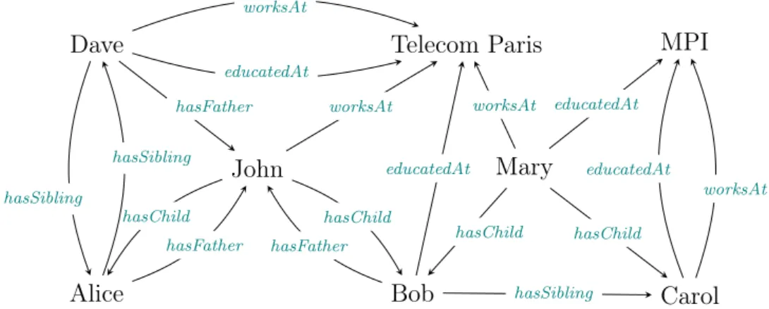
Example 2.19. Consider the knowledge base shown in Figure 2.2 with an empty TBox. Consider the rules r1 and r2:

r1(x, y) : ∃z worksAt (x, z) ∧ educatedAt (y, z) → hasChild (x, y)

r2(x, z) : ∃y hasFather (x, y) ∧ hasChild (y, z) → hasSibling(x, z)

The first rule states that workers of certain institutions often have children among the people educated there. The second rule states that if your father has children, then they are your siblings.

(27)

John Mary

Alice Bob Carol

Dave Telecom Paris MPI

worksAt worksAt educatedAt hasChild hasChild hasChild hasFather hasChild hasFather educatedAt educatedAt worksAt hasFather hasSibling hasSibling worksAt educatedAt hasSibling

The body of r1 seen as a query, b1(x, y) = ∃z worksAt (x, z) ∧ educatedAt (y, z),

has 8 possible answers in K: (Dave, Dave), (Dave, Bob), (John, Dave)... Hence, the body support of the rule r1 is supp(b1(x, y)) = 8. The only two possible answers

of the query b1(x, y) ∧ hasChild (x, y) are (John, Bob) and (Mary, Bob). Hence

supp(r1) = 2. So, have conf (r1) = 2₈.

Analogously, for r2, b2(x, z) = ∃y hasFather (x, y) ∧ hasChild (y, z) has 6 answers

and therefore supp(b2(x, z)) = 6. However, only one of these answers is such that

hasSibling(x, z) holds, so supp(r2) = 1. This leads to conf (r2) = 1₆.

Support and confidence were originally developed for scoring rules over complete data. If data is missing, their interpretation is not straightforward and they can be misleading. For example, in Example 2.19, the rule r1 has a confidence of 1₄

and r2 has a lower confidence of 1₆, although r1 is clearly wrong.

The reason is that the standard confidence aims first at avoiding wrong asser-tions in the predicasser-tions. It does so by considering as wrong all predicted asserasser-tions that are not already in the knowledge base, even if these assertions might be true in the real world. Other approaches aim at finding other compromises between predicting wrong facts and missing true facts. In Galárraga, Teflioudi, et al., 2015, the confidence under the Partial Completeness Assumption (PCA) has been pro-posed as a measure. This measure guesses negative facts by assuming that data is usually added to knowledge bases in batches. For example, if at least one child of John is known then most probably all of John’s children are present in the knowledge base.

Definition 2.20 (PCA confidence). The PCA confidence is defined for all rules of the form r(x, y) : b(x, y) → h(x, y) where x and y are variables and h a role assertion by:

(28)

confpca(r) :=

supp(r) supppca(r)

where

supppca(r) := |{(x, y) | K |= b(x, y) and ∃y0 ∈ NIK |= h(x, y0)}|

Example 2.21. We obtain confpca(r1) = 2₄. Indeed, since Carol and Dave are not

known to have any children in the knowledge base, four existing body substitutions are not counted in the denominator. Meanwhile, we have confpca(r2) = 1₆, since

all people that are predicted to have siblings by r2 already have siblings in the

available knowledge base. Knowledge base completion

After having mined rules, we want to use them to complete the knowledge base. That is, we want to add to the knowledge base all the assertions that are generated by the rules. Formally:

Definition 2.22 (Rule-based knowledge base completion). Let K be a knowledge base and let r be a rule such that r(~x) = b(~x) → h1(~x) ∧ · · · ∧ hn(~x) where the

hi are concept or role assertions. Then the completion of K = (A, T ) by r is a

knowledge base Kr = (Ar, T ) such that Ar = A ∪ {h1(~a), . . . , hn(~a) | K |= b(~a)}.

Example 2.23. If we follow Example 2.19, we have Aa

r1 = A ∪ { hasChild (John,

Dave), hasChild (Carol, Mary), hasChild (Dave, Dave), hasChild (Carol, Carol), hasChild (Dave, Bob), hasChild (Mary, Dave) }.

Note that the ideal knowledge base Ki _{introduced in Section 2.1 is the perfect}

completion of Ka_{, i.e., it is supposed to contain all correct facts with entities and}

relations from ΣKa that hold in the current state of the world. The goal of

rule-based knowledge base completion is to extract from Ka _{a set of rules R such that}

∪r∈RKar is as close to Ki as possible.

Rule evaluation

To evaluate the predictions of a rule r(~x) : b(~x) → h(~x) against a set of expected predictions P, we can use the following metrics:

Definition 2.24 (Precision). The precision of a rule is the fraction of the predic-tions computed by the rule that are in the set of expected predicpredic-tions P. This measure aims at computing how many of the rule predictions are expected predic-tions. Formally:

precision(r) := |{~x | K |= b(~x) ∧ P |= h(~x)}| |{~x | K |= b(~x)}|

(29)

Definition 2.25 (Recall). The recall is given by the fraction of the predictions computed by the rule r that are in the set of expected predictions P. This measure aims at computing how many of the expected predictions are found by the rules. Formally:

recall (r) := |{~x | K |= b(~x) ∧ P |= h(~x)}| |{~x | P |= h(~x)}|

Definition 2.26 (F1 score). The F1 score is the harmonic mean of precision and recall:

F1(r) := 2

precision(r) · recall (r) precision(r) + recall (r)

Example 2.27. Consider the same knowledge base and rules as in Example 2.19. We evaluate the rule r1 against the expected prediction set:

P = { hasChild (John, Dave), hasChild (John, Alice), hasChild (John, Bob), hasChild (Mary, Bob), hasChild (Mary, Carole), hasChild (Mary, Dave) } Like presented in Example 2.19, r1 predicts 8 facts. In these facts 4 are

in P: hasChild (John, Dave), hasChild (John, Bob), hasChild (Mary, Bob), and hasChild (Mary, Dave).

Hence we have precision(r1) = 4₈ = 0.5 and recall (r1) = 4₆ = 0.66. This gives

us F1(r1) = 2_0.5+0.660.5·0.66 = 0.57.

Now that we have the preliminaries in place, we will move to the first contri-bution of this thesis. This contricontri-bution aims at refining the confidence measure when cardinality information is available in the knowledge base.

(30)

Part I

(31)

(32)

Chapter 3 Completeness-aware Rule Scoring

The work presented in this chapter has been done with Daria Stepanova, Simon Razniewski, Paramita Mirza and Gerhard Weikum and has been published at ISWC 2017. It was one of the papers nominated for the best student paper award. An invited short version of the paper has been published at IJCAI 2018.1

Thomas Pellissier Tanon, Daria Stepanova, Simon Razniewski, Paramita Mirza, and Gerhard Weikum. “Completeness-Aware Rule Learning from Knowledge Graphs”. Full paper at ISWC 2017. https://doi.org/10. 1007/978-3-319-68288-4_30

Thomas Pellissier Tanon, Daria Stepanova, Simon Razniewski, Paramita Mirza, and Gerhard Weikum. “Completeness-aware Rule Learning from Knowledge Graphs”. Invited paper at IJCAI 2018. https://doi.org/ 10.24963/ijcai.2018/749

3.1 Introduction

Motivation

An important task over knowledge bases is rule learning. This task aims at learn-ing new rules on the knowledge base. For example, the rule r1 : worksAt (x, z) ∧

educatedAt (y, z) → hasChild (x, y) could be mined from the knowledge base dis-played in Figure 3.1 page 36. This rule states that workers of certain institutions often have children among the people educated there, as this is frequently the 1_{Some rule quality measures presented in the ISWC paper are omitted here to focus on my}

(33)

case for popular scientists. Rules are relevant for a variety of applications rang-ing from knowledge base curation, e.g., completion and error detection (Paulheim, 2017; Galárraga, Teflioudi, et al., 2015; Gad-Elrab et al., 2016), to data mining and semantic culturonomics (Suchanek and Preda, 2014). Section 2.3 Page 22 has formally defined the concept of rules and presented some existing methods to evaluate them.

However, since such rules are learned from incomplete data, they might be erroneous and might make incorrect predictions on missing facts. The already presented rule r1 is clearly not universal and should be ranked lower than the rule

r2 : hasFather (x, y) ∧ hasChild (y, z) → hasSibling(x, z). However, standard rule

measures like confidence (i.e., the conditional probability of the rule’s head given its body) incorrectly favor r1 over r2 for the given knowledge base.

Recently, efforts have been put into detecting the concrete number of facts of certain types that hold in the real world (e.g., “Einstein has 3 children”) by exploiting Web extraction and crowd-sourcing methods (Mirza, Razniewski, and Nutt, 2016; Prasojo et al., 2016). Such cardinality information provides a lot of hints about the topology of knowledge bases and reveals parts that should be especially targeted by rule learning methods. It can also give hints to detect bad rules. For example, r1 is probably going to create too many facts to comply with

cardinality hints like “a person has at most two parents”. However, surprisingly, despite its obvious importance, to date, no systematic way of making use of such information in rule learning exists.

In this chapter, we propose to exploit cardinality information about the ex-pected number of edges in knowledge bases to better assess the quality of learned rules. Because knowledge bases are often incomplete in some areas and complete in others, our intuition is that some cardinality information might help to assess rules quality, at least by discarding rules which add facts in already complete areas like suggested earlier.

State of the art and its limitations

Galárraga, Teflioudi, et al., 2013 introduced a completeness-aware rule scoring based on the partial completeness assumption (PCA). The idea of the partial completeness assumption is that if at least one object for a given subject and a predicate is in a knowledge base (e.g., “Eduard is Einstein’s child”), then all objects for that subject-predicate pair (“Einstein’s children”) are assumed to be known. This assumption was taken into account in rule scoring, and empirically it turned out to be indeed valid in real-world knowledge bases for some topics. However, it does not universally hold and does not correctly handle the case when edges in a graph are missing in a seeminlgy random fashion. For example, in encyclopedic knowledge bases like Wikidata, only well-known children are present in the

(34)

knowl-edge base, and not the less famous ones or the ones who died in their infancy. It is also the case for relations with no well-defined cardinalities, like “award received” or “position held”. Often, only the most prominent values are provided for this relation. Similarly, Doppa et al., 2011 discussed the absence of contradiction as confirmation for “default” rules, i.e., rules that hold in most cases, leading the few contradicting facts to be highlighted and better covered in the knowledge base. Galárraga, Razniewski, et al., 2017 used crowd-sourcing to acquire completeness data. The acquired statements were then used in a post-processing step of rule learning to filter out predictions that violate these statements. However, this kind of filtering does not have any impact on the quality of the mined rules and the incorrect predictions for instances about which no completeness information exists. Contributions

This work presents the first proper investigation of how cardinality information, and more specifically the number of edges that are expected to exist in the real world for a given subject-predicate pair in a knowledge base, can be used to improve rule learning. The contributions of our work are as follows:

• We present an approach that accounts for sparse data about the number of edges that should exist for given subject-predicate pairs in the ranking stage of rule learning. This is done by introducing a new ranking measure, the completeness confidence. This confidence generalizes both the standard con-fidence and the PCA concon-fidence. Specifically, it performs identically to the two existing confidence measures if the corresponding cardinality metadata are provided. For example, if the knowledge base is stated to be globally complete, our completeness confidence will be the same as standard confi-dence, so it will also have the same performance.

• We implement our new ranking measure and evaluate it both on real-world and synthetic datasets, showing that they outperform existing measures both with respect to the quality of the mined rules and the predictions they pro-duce.

3.2 Related Work

Rule learning

The problem of automatically learning patterns from knowledge bases has gained a lot of attention in recent years. Some relevant works are Galárraga, Teflioudi, et al., 2013; Galárraga, Teflioudi, et al., 2015; Zhichun Wang and Li, 2015, which focus on learning Horn rules and either ignore completeness information or make

(35)

use of completeness by filtering out predicted facts violating completeness in a post-processing step. On the contrary, we aim at injecting the statements into the learning process.

In the association rule mining community, some works focused on finding (in-teresting) exception rules, which are defined as rules with low support (rare) and high confidence (e.g., Taniar et al., 2008). Our work differs from this line of re-search because we do not necessarily look for rare interesting rules, but care about the quality of their predictions.

Another relevant stream of research is concerned with learning Description Logic TBoxes or schema (e.g., Lehmann et al., 2011). However, these techniques focus on learning concept definitions rather than nonmonotonic rules. The main difference between us and these approaches is that we aim at finding a hypothesis that consistently predicts unseen data, while DL learners focus more on learning models that perfectly describe the data.

In the context of inductive and abductive logic programming, learning rules from incomplete interpretations given as a set of positive facts along with a pos-sibly incomplete set of negative ones was studied, e.g., in Law, Russo, and Broda, 2014. In contrast to our approach, this work does not exploit knowledge about the number of missing facts, and neither do the works on terminology induction, e.g., Sazonau, Uli Sattler, and Brown, 2015. Learning nonmonotonic rules in the pres-ence of incompleteness was studied in hybrid settings (Józefowska, Lawrynowicz, and Lukaszewski, 2010; Lisi, 2010), where a background theory or a hypothesis can be represented as a combination of an ontology and Horn or nonmonotonic rules. The main point in these works is the assumption that there might be potentially missing facts in a given dataset. However, it is not explicitly mentioned which parts of the data are (in)complete like in our setting. Moreover, the emphasis of these works is on the complex reasoning interaction between the components, while we are more concerned with techniques for deriving rules with high predictive quality from large knowledge bases. The work by d’Amato et al., 2016 ranks rules using the ratio of correct versus incorrect predictions. These incorrect predictions are found using ontologies that allow determining incorrect facts. In contrast to our scenario of interest, in their work, the knowledge about the exact numbers of missing knowledge base facts has not been exploited. Since the publication of our original paper, Ho et al., 2018 presented an approach using numerical embeddings to predict possible missing facts. The authors used these predicted missing facts to refine the scoring of rules in incomplete areas. Muñoz, Minervini, and Nick-les, 2019 used cardinality information to refine the learning of entity numerical embeddings to better predict facts missing in the knowledge base.

There are also many less relevant statistical approaches to completing knowl-edge bases based on, e.g., low-dimensional embeddings (Zhen Wang et al., 2014)

(36)

or tensor factorization (Nickel, Tresp, and Kriegel, 2012). Completeness information

The idea of bridging the open and closed world assumption by using completeness information was first introduced in the database world in Levy, 1996; Etzioni, Golden, and Weld, 1997, and later adapted to the Semantic Web in Darari, Nutt, et al., 2013. For describing such settings, the common approach is to fix the complete parts (and assume that the rest is potentially incomplete).

Galárraga, Razniewski, et al., 2017 have extended the rule mining system AMIE to mine rules that predict where a knowledge base is complete or incomplete. The focus of the work is on learning association rules like “If someone has a date of birth but no place of birth, then the place of birth is missing.” In contrast, we reason about the missing edges by trying to estimate the exact number of edges that should be present in a knowledge base. In Galárraga, Razniewski, et al., 2017 it has also been shown that completeness information can be used to improve the accuracy of fact prediction, by pruning out in a post-processing step those facts that are predicted in parts expected to be complete. In the present chapter, we take a more direct approach and inject completeness information already into the rule acquisition phase, to also prune away problematic rules, not only individual wrong predictions.

Our cardinality statements (e.g., “John has 3 children”) encode knowledge about parts of a knowledge base that are (un)known, and thus should have points of contact with operators from epistemic logic; we leave the extended discussion on the matter for future work.

3.3 Approach

In the following we make the unique name assumption, i.e., we assume that each entity is represented by at most one individual (Definition 2.9 Page 20). We also use the distinction between ideal knowledge base and available knowledge base presented in Section 2.1 Page 21.

We use here all the definitions related to knowledge bases and rules presented in the preliminaries (Chapter 2). We also assume that the rule head contains a single role assertion h(x, y). This does not introduce a loss of generality compared to rules with a conjunction of role assertions in the head because rules under the form b(~x) → h1(~x) ∧ · · · ∧ hn(~x) could be converted into an equivalent set of rules

b(~x) → h1(~x), . . . , b(~x) → hn(~x).

Scoring and ranking rules are core steps in association rule learning. A variety of measures for ranking rules have been proposed, with prominent ones being

(37)

confidence (Definition 2.20 Page 24), conviction (Brin et al., 1997), and lift2_.

The existing (in-)completeness-aware rule measure in the knowledge base con-text, the PCA confidence from Galárraga, Teflioudi, et al., 2015, already presented in Definition 2.20 Page 24, has two apparent shortcomings: First, it only counts as counterexamples those pairs (x, y) for which at least one h(x, y0) is in the current available knowledge base Kafor some y0 and a rule’s head predicate h. This means it may incorrectly give high scores to rules predicting facts for very incomplete relations, e.g., place of baptism. Second, it is not suited to relations that are not added in a “none or all” matter. For example, the most important values of an “awards” relation are often known, while the other values are often unknown or added to the knowledge base much later.

Thus, in this work, we focus on the improvements of rule scoring functions by making use of extra cardinality information. Before dwelling into the details of our approach we discuss the formal representation of such cardinality statements.

Cardinality Statements Overall, one can think of 4 different cardinality tem-plates obtained by fixing the subject or object in a role assertion or considering a concept assertion and reporting the number of respective facts that hold in Ki_.

E.g., for hasChild (John, Mary) we can count (1) the children of John; (2) the peo-ple of which Mary is a child of; or (3) the facts over hasChild relation. And for Person(John) we can count (4) the number of elements in the Person concept.

In practice, numerical statements for templates (1), (2), and (4) can be obtained using web extraction techniques (Mirza, Razniewski, and Nutt, 2016), from func-tional properties of relations, from closed concepts, or from crowd-sourcing. For (3) things get trickier. We leave this issue for future work and focus here only on tem-plates (1), (2), and (4). We work in the following only on template (1). Indeed, we can rewrite (2) to (1) provided that inverse relations can be expressed in a knowl-edge base. For instance, |{s | hasChild (s, john)}| = |{o | hasParent (john, o)}| for the predicates hasChild and hasParent , which are inverses of one another. More, it is possible to rewrite (4) to (1) with some notation abuse by writing hasInstance(C, o) the concept assertion C(o).

We have now a simple way to report (the numerical restriction on) the absolute number of facts over a certain roles in the ideal knowledge base Ki_{. To formalize}

it, we define the partial function num that takes as input a role p ∈ NR and an

individual s ∈ NI and outputs a natural number corresponding to the number of

facts in Ki _{over p with s as the first argument:}

num(p, s) := |{o | Ki |= p(s, o)}| (3.1)

2_{The lift of a rule r(~}_{x) = b(~}_{x) → h(~}_{x) is defined by lift (r) =} supp(b∧h) supp(b)·supp(h).

(38)

num is a partial function because most of the time we do not know all cardinalities. For example, in a knowledge base about some people’s family, the number of biological parents is always known whereas it might be the case that the number of children is known for some people only and the number of siblings is never known.

Naturally, the number of missing facts for a given p and s can be obtained as miss(p, s) := num(p, s) − |{o | Ka |= p(s, o)}| (3.2) Example 3.1. Consider the knowledge base in Figure 3.1 (the same one as the knowledge base presented in the preliminaries) and the following cardinality state-ments for it:

num(hasChild,John) = 3 num(hasChild, Mary) = 3 num(hasChild, Alice) = 1 num(hasChild, Carol) = 0 num(hasChild, Dave) = 0 num(hasSibling, Bob) = 3 num(hasSibling, Alice) = 2 num(hasSibling, Carol) = 2 num(hasSibling, Dave) = 2 We then have:

miss(hasChild , Mary) = miss(hasChild , John) = miss(hasChild , Alice) = 1; miss(hasChild , Carol) = miss(hasChild , Dave) = 0;

miss(hasSibling, Bob) = miss(hasSibling, Carol) = 2; miss(hasSibling, Alice) = miss(hasSibling, Dave) = 1.

We are now ready to define the completeness-aware rule scoring problem. Given a knowledge base and a set of cardinality statements, completeness-aware rule scor-ing aims to score rules not only by their predictive power on the known knowledge base like presented in Section 2.3 Page 22, but also with respect to the number of wrongly predicted facts in complete areas and the number of newly predicted facts in known incomplete areas.

In this work, we propose to explicitly rely on incompleteness information to determine whether to consider an assignation as a counterexample for a rule at hand or not.

To do that, we first define two indicators for a given rule r, reflecting the number of new predictions made by r in incomplete (npi (r)) and, respectively, complete (npc(r)) knowledge base parts:

(39)

John Mary

Alice Bob Carol

Dave Telecom Paris MPI

worksAt worksAt educatedAt hasChild hasChild hasChild hasFather hasChild hasFather educatedAt educatedAt worksAt hasFather hasSibling hasSibling worksAt educatedAt hasSibling

Definition 3.2. The Number of Predictions in Incomplete parts of a rule r(x, y) = b(x, y) → h(x, y) is the number of new predictions of r that add objects in the places where it is known that values are missing. It is formally defined by:

npi (r) := X

x∈NIand miss(h,x) is defined

min(pred (r, x), miss(h, x))

where pred (r, x) is the number of new predictions of r for a given x: pred (r, x) := |{y | Ka |= b(x, y) ∧ Ka 6|= h(x, y)}|

Definition 3.3. Similarly, the Number of Predictions in Complete parts of a rule r(x, y) = b(x, y) → h(x, y) is the number of new predictions of r that add objects in the places where it is known that miss(h, x) objects are missing and the rules already predicted miss(h, x) other objects. It is formally defined by:

npc(r) := X

x∈NIand miss(h,x) is defined

max (pred (r, x) − miss(h, x), 0)

where pred (r, x) is the number of new predictions of r for a given x: pred (r, x) := |{y | Ka|= b(x, y) ∧ Ka_{6|= h(x, y)}}

Example 3.4. Consider the knowledge base whose ABox is displayed in Figure 3.1 with an empty TBox, and the cardinality statements described in Example 3.1.

We consider the rules:

(40)

r2 : hasFather (x, y) ∧ hasChild (y, z) → hasSibling(x, z)

r1 predicts new hasChild values for Carol, Dave, John, and Mary. Among them,

the expected cardinality is only known for Carole and Dave.

The two predicted assertions for Carol are hasChild (Carol, Carol) and hasChild (Carol, Mary). Among them, none is already in the knowledge base so pred (r1, Carol) = 2. With a similar reasoning, we get pred (r1, Dave) = 2.

The two predicted assertions for John are hasChild (John, Dave) and has-Child (John, Bob). However hashas-Child (John, Bob) is already in the knowledge base so pred (r1, John) = 1. In the same way, we get pred (r1, Mary) = 1.

Because miss(hasChild, Carol) = 0, miss(hasChild, Dave) = 0, miss(hasChild, John) = 1, and miss(hasChild, Mary) = 1, we have npi (r1) = min(2, 0)+min(2, 0)+

min(1, 1) + min(1, 1) = 2 and npc(r1) = max (2 − 0, 0) + max (2 − 0, 0) + max (1 −

1, 0) + max (1 − 1, 0) = 4.

Similarly, we get npi (r2) = 4 and npc(r2) = 1.

Exploiting these additional indicators for r(x, y) : b(x, y) → h(x, y) we obtain the following completeness-aware confidence:

Definition 3.5. The completeness-aware confidence confidence is defined by: confcomp(r) :=

supp(r) supp(b) − npi (r)

Example 3.6. We consider the same knowledge base and rules as Example 3.4. Obviously, the rule r2 should be preferred over r1.

The body and rule supports of r1 over the knowledge base are supp(b1) = 8

and supp(r1) = 2 respectively. Hence, we have conf (r1) = 2₈ and conf (r2) = 1₆.

As discussed before, we obtain confpca(r1) = 2₄. Indeed, since Carol and Dave

are not known to have any children in the knowledge base, four existing body sub-stitutions are not counted in the denominator. Meanwhile, we have confpca(r2) = 1₆,

since all people that are predicted to have siblings by the rule already have siblings in the available knowledge base Ka.

For our completeness confidence, confcomp(r1) = ₈₋₂2 = 2₆ and confcomp(r2) = 1

6−4 = 1

2, resulting in the desired rule ordering, which is not achieved by existing

measures.

Our completeness confidence generalizes both the standard and the PCA con-fidence. Indeed, under the Closed World Assumption, the knowledge base is sup-posed to be fully complete, i.e., for all p ∈ NR, s ∈ NI we have miss(p, s) = 0.

Similarly, if we assume the Partial Completeness Assumption, then for all pairs p, s such that at least one o ∈ NI exists with Ka |= p(s, o), miss(p, s) = 0 and

(41)

Proposition 3.7. For every knowledge base K and rule r it holds that (i) under the Closed World Assumption (CWA) confcomp(r) = conf (r);

(ii) under the Partial Completeness Assumption (PCA) confcomp(r) = confpca(r).

Proof. (i) Under the Closed World Assumption, it holds that for all p ∈ NR,

s ∈ NI, miss(p, s) = 0. Thus, for all rules r, we have that npi (r) = 0, and hence,

confcomp(r) = conf (r).

(ii) Under the Partial Completeness Assumption, it is assumed that for all p ∈ NR

and s ∈ NI it holds that miss(p, s) = 0 if ∃o Ka |= p(s, o) and miss(p, s) = +∞ if

not. Hence, for all r we have npi (r) =P

xpredict (r, x), where

predict (r, x) = (

0, if ∃y Ka |= h(x, y)

pred (r, x), if ∀y0Ka _{6|= h(x, y}0₎

From this we get confcomp(r) =

supp(r) supp(b) −P

x such that ∀y0_Ka_6|=h(x,y0₎pred (r, x)

The denominator of the latter formula counts all matches of the rule body and subtracts from them those for which the head h(x, y) is predicted and ∀y0 Ka _6|=

h(x, y0). Hence, we end up counting only body substitutions with Ka _{|= h(x, y}0₎

for at least one y0, i.e., |{(x, y) | ∃y Ka_{|= b(x, y) ∧ ∃y}0_Ka _{|= h(x, y}0_{)}| = supp} pca(r).

Hence, confcomp(r) = _suppsupp(r)_pca_(r) = confpca(r).

3.4 Evaluation

We have implemented our completeness-aware rule learning approach into a C++ system prototype CARL3_{, following a standard relational learning algorithm}

im-plementation such as Goethals and Bussche, 2002. While our general methodology can be applied to mining rules of arbitrary form, in the experimental evaluation to restrict the rule search space we focus only on rules with two atoms in their body of the form

p(x, y) ∧ q(y, z) → r(x, z) (3.3)

Note that here p, q, and r are not allowed to denote inverse property expres-sions. We aim to compare the predictive quality of the top k rules mined by our completeness-aware approach with the ones learned by standard rule learning

(42)

methods: (1) the PCA confidence (Definition 2.20 Page 24) from AMIE (Galár-raga, Teflioudi, et al., 2015) and (2) the standard confidence (Definition 2.18 Page 23) used e.g., by WarmeR (Goethals and Bussche, 2002).

Because the goal of our new confidence is to provide a better rule quality evaluation measure, we only compare with other rule quality measures that have already proved their quality and usefulness, and we do not compare with fact prediction approaches or with baselines.

Dataset

We used two datasets for the evaluation: (i) WikidataPeople, which is a dataset we have created from the Wikidata knowledge base, containing 2.4M facts over 9 pred-icates4 _{about biographical information and family relationships of people; and (ii)}

LUBM, which is a synthetic dataset describing the structure of a university (Guo, Pan, and Heflin, 2005).

For the WikidataPeople dataset, the approximation of the ideal knowledge base (Ki) is obtained by exploiting available information about inverse rela-tions (e.g., hasParent is the inverse of hasChild ), functional relarela-tions (e.g., hasFather , hasMother ) as well as manually hand-crafted solid rules from the family domain like

hasParent (x, z) ∧ hasParent (y, z) ∧ x 6= y → hasSibling(x, y).5

We generated cardinality statements from WikidataPeople Ki _{by exploiting}

properties of functional relations, e.g., hasBirthPlace, hasFather , hasMother must be uniquely defined. We considered also that everybody with a hasDeathDate has a hasDeathPlace. For the other relations, the PCA (Galárraga, Teflioudi, et al., 2015) is used. This resulted in 10M cardinality statements.

LUBM Ki_{, with 1.2M facts, was constructed by running the LUBM data}

gen-erator for 10 universities, removing all rdf:type triples, and introducing inverse predicates. 464K cardinality statements were obtained by counting the number of existing objects for each subject-predicate pair after completing the graph using the provided OWL ontology, i.e., assuming the partial completeness assumption on the whole dataset.

Experimental Setup

To assess the effect of our proposed measures, we first construct versions of the available knowledge base (Ka_{) by removing parts of the data from K}i_and

introduc-ing a synthetic bias in the data (i.e., leavintroduc-ing many facts in Ka for some relations 4_{hasFather , hasMother , hasStepParent , hasSibling, hasSpouse, hasChild , hasBirthPlace,}

hasDeathPlace, and hasNationality

(43)

and few for others). The synthetic bias is needed to simulate our scenario of inter-est, where some parts of Ka are very incomplete while others are fairly complete, which is indeed the case in real-world knowledge bases. In Wikidata, for instance, sibling information is only reported for only 3% of non-living people, while children data is known for 4%.

For that, we proceed in two steps: First, we define a global ratio, which deter-mines a uniform percentage of data retained in the available graph. This ra-tio is useful to check how the different measures perform with respect to the (in-)completeness of the knowledge base. To further refine this, we then define a predicate ratio individually for each predicate to simulate the real world discrep-ancies between fairly complete and very incomplete areas. For the WikidataPeople knowledge base, this ratio is chosen as (i) 0.8 for hasFather and hasMother ; (ii) 0.5 for hasSpouse, hasStepParent , hasBirthPlace, hasDeathPlace and hasNationality; (iii) 0.2 for hasChild ; and (iv) 0.1 for hasSibling. For the LUBM dataset, the predicate ratio is uniformly defined as 1 for regular predicates and 0.5 for inverse predicates. Note that this static predicate ratio is here to simulate the complete-ness gap in the knowledge base between predicates. Hence, the predicate ratio is fixed as part of the design of the experimental setup, and we do not make it vary or otherwise study it in our experimental results

For a given predicate, the final ratio of facts in Ka _{retained from those in K}i

is then computed as min(1, 2 · k · n), where k is the predicate ratio and n is the global ratio.

Note that, after randomly removing facts, the partial completeness assump-tion no longer holds on the data. This gives our method a competitive edge over competing approaches such as AMIE which assume the partial completeness as-sumption.

The assessment of the rules learned from different versions of the available knowledge base is performed by comparing rule predictions with the approximation of Ki_{. More specifically, every learned rule is assigned a quality score, defined as}

the ratio of the number of predictions made by the rule in Ki\ Ka _{over the number}

of all predictions outside Ka.

qualityScore(r) = |K a r∩ Ki\ Ka| |Ka r \ Ka| (3.4)

This scoring naturally allows us to control the percentage of rule predictions that hit our approximation of Ki_{, similar to standard recall estimation in machine}

(44)

0.2 0.3 0.4 0.5 0.6 0.7 0.8 0.9 1K 2K 3K 4K 5K 6K

Global ratio of the available KB

A v erage supp ort 10 20 30 40 50 Num b er of k ept rules #Rules (WikidataPeople) #Rules (LUBM)

Avg. support (WikidataPeople) Avg. support (LUBM)

Figure 3.2 – Number of kept rules and their average support for WikidataPeople and LUBM datasets 0.2 0.4 0.6 0.8 1 0 0.2 0.4 0.6 0.8 1

Global ratio of the available KB

P earson correlation WikidataPeople 0.2 0.4 0.6 0.8 1 0 0.2 0.4 0.6 0.8 1

Global ratio of the available KB LUBM

Standard confidence PCA confidence

Completeness confidence

(45)

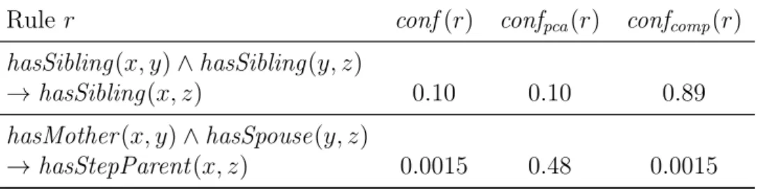
Table 3.1 – Example of a good and a bad rule mined from WikidataPeople with global ratio of 0.5

Rule r conf (r) confpca(r) confcomp(r)

hasSibling(x, y) ∧ hasSibling(y, z)

→ hasSibling(x, z) 0.10 0.10 0.89

hasMother (x, y) ∧ hasSpouse(y, z)

→ hasStepParent (x, z) 0.0015 0.48 0.0015

Results

From every version of the available knowledge base, we have mined all possible rules with two atoms in their body of the form of Equation 3.3 (page 38). For that, we search all the possible tuples (p, q, r) such that the conjunctive query (x, y)∧q(y, z)∧r(x, z) has at least one answer. We kept only rules r with conf (r) ≥ 0.001 and supp(r) ≥ 10, whose head coverage6 _{is greater than 0.001. Figure 3.2}

shows the number of kept rules and their average support (Definition 2.17 Page 23) for each global ratio used for generating Ka_.

The evaluation results for WikidataPeople and LUBM datasets are in Fig-ure 3.3. The horizontal axis displays the global ratio used for generating Ka_{. We}

compared different rule ranking methods as previously discussed. The Pearson correlation coefficient (vertical axis) between each ranking measure and the qual-ity score of rules (Equation 3.4) is used to evaluate the measures’ effectiveness. The Pearson correlation coefficient between two random variables X and Y with numerical values is defined by ρX,Y = cov (X,Y )_σ

XσY with cov being the covariance and

σ the standard deviation. We measured the Pearson correlation coefficient since apart from the ranking order (as captured by, e.g., Spearman’s rank correlation coefficient), the absolute values of the measures are also insightful for our setting. Since facts are randomly missing in the considered versions of Ka, the PCA confidence performs worse than the standard confidence for given datasets, while our completeness confidence significantly outperforms both (see Table 3.1 for ex-amples).

For both knowledge bases, the completeness confidence outperforms the rest of the measures. It is noteworthy that the standard confidence performs considerably better on the LUBM knowledge base with a correlation coefficient higher than 0.9 than on the WikidataPeople knowledge base. Still, completeness confidence shows better results, reaching a nearly perfect correlation of 0.99. We hypothesize that 6_{Head coverage is the ratio of the number of predicted facts that are in K}a _{over the number}

(46)

this is due to the bias between the different predicates of the LUBM knowledge base being less strong than in the WikidataPeople knowledge base, where some predicates are missing a lot of facts, while others just a few.

3.5 Conclusion

We have defined the problem of learning rules from incomplete knowledge bases enriched with the exact numbers of missing edges of certain types. We proposed a novel rule ranking measure that effectively makes use of sparse cardinality informa-tion, the completeness confidence. Our new measure has been injected in the rule learning prototype CARL and evaluated on real-world and synthetic knowledge bases, demonstrating significant improvements both with respect to the quality of mined rules and with respect to the predictions they produce.

For future work, it would interesting to expend the experiments. We could benchmark our completeness confidence against Galárraga, Razniewski, et al., 2017 to check which method produces the best predictions and which has the best runtime. We could also adapt the AMIE rule learning algorithm to make it work with our completeness confidence instead of the PCA confidence.

(47)

(48)

Chapter 4 Increasing the Number of Numerical

Statements

The work presented in this chapter has been done with Daria Stepanova, Simon Razniewski, Paramita Mirza, and Gerhard Weikum and has been published at ISWC 2017 alongside the previous chapter content.

Thomas Pellissier Tanon, Daria Stepanova, Simon Razniewski, Paramita Mirza, and Gerhard Weikum (2017). “Completeness-Aware Rule Learning from Knowledge Graphs”. In: ISWC, pp. 507–525. https://doi.org/ 10.1007/978-3-319-68288-4_30

4.1 Introduction

We have shown in the previous chapter that the exploitation of numerical com-pleteness statements is beneficial for rule quality assessment. A natural question is where to acquire such statements in real-world settings. Like already men-tioned in the previous chapter, various works have shown that numerical asser-tions can be frequently found on the Web (Darari, Nutt, et al., 2013), obtained via crowd-sourcing (Darari, Razniewski, et al., 2016), text mining (Mirza, Razniewski, Darari, et al., 2017), or even using Hoeffding’s inequality to find upper bounds (Gi-acometti, Markhoff, and Soulet, 2019). Other work like Galárraga, Razniewski, et al., 2017 aims at mining if the knowledge base is complete for a given subject and predicate, a much more restricting set that mining the actual (in-)completeness statement. We believe that mining numerical correlations concerning knowledge base edges and then assembling them into rules is a valuable and a modular ap-proach to increase the amount of completeness information, which we present in

Knowledge base curation using constraints

HAL Id: tel-03102638

https://tel.archives-ouvertes.fr/tel-03102638

Knowledge base curation using constraints

Thomas Pellissier-Tanon

To cite this version:

NNT

:

2020IPP

A

T025

Knowledge Base Curation

using Constraints

T

HOMAS

P

ELLISSIER

T

ANON

Knowledge Base Curation using Constraints

Thomas Pellissier Tanon

September 7th, 2020

Abstract

Remerciements

Contents

I

Mining Constraints

27

II

Enforcing Constraints Statically

51

III

Enforcing Constraints Dynamically

71

Chapter 1

Introduction

1.1

Motivation

1.2

Presented Contributions

1.3

Other works

Chapter 2

Preliminaries

2.1

Knowledge bases

2.2

Queries

2.3

Rules and Rule Learning

Part I

Chapter 3

Completeness-aware Rule Scoring

3.1

Introduction

3.2

Related Work

3.3

Approach

3.4

Evaluation

3.5

Conclusion

Chapter 4

Increasing the Number of Numerical

Statements

4.1

Introduction