1
QUANTIFYING INPUT-UNCERTAINTY IN 2
TRAFFIC ASSIGNMENT MODELS 3
4 5
Konstantinos Perrakisa, Mario Coolsb,c, Dimitris Karlisd, Davy Janssensa , 6
Bruno Kochana, Tom Bellemansa and Geert Wetsa,* 7
8
a
Transportation Research Institute 9 Hasselt University 10 Wetenschapspark 5, bus 6 11 BE-3590 Diepenbeek 12 Belgium 13 Fax.:+32(0)11 26 91 99 14 Tel:+32(0)11 26 91{40, 28, 47, 27, 58} 15
Email: {konstantinos.perrakis, davy.janssens, 16
bruno.kochan, tom.bellemans, geert.wets}@uhasselt.be 17
18
b
Centre for Information, Modeling and Simulation (CIMS) 19 Hogeschool-Universiteit Brussel 20 Warmoesberg 26 21 BE-1000 Brussels 22 Belgium 23 Tel: +32(0)479 52 62 99 24 Email: [email protected] 25 26 c
Research Foundation Flanders (FWO) 27 Egmontstraat 5 28 BE-1000 Brussels 29 Belgium 30 31 d Department of Statistics 32
Athens University of Economics and Business 33 76 Patision Str, 10434, Athens 34 Greece 35 Tel:+30 210 8203920 36 Email: [email protected] 37 38 Number of words: 6239 39 Number of Tables: 1 40 Number of Figures: 4 41
Total number of words: 6239 + 5*250 = 7489 42
43
Revised paper submitted: November 13, 2011 44
45
* Corresponding author 46
ABSTRACT 1
2
Traffic assignment methods distribute Origin-Destination (OD) flows throughout the links of a 3
given network according to procedures related to specific deterministic or stochastic modeling 4
assumptions. In this paper, we propose a methodology that enhances the information provided 5
from traffic assignment models, in terms of delivering stochastic estimates for traffic flows on 6
links. Stochastic variability is associated to the initial uncertainty related to the OD matrix used 7
as input into a given assignment method, and therefore the proposed methodology is not 8
constrained by the choice of the assignment model. The methodology is based on Bayesian 9
estimation methods which provide a suitable working framework for generating multiple OD 10
matrices from the corresponding predictive distribution of a given statistical model. Predictive 11
inference for link flows is then straightforward to implement, either by assigning summarized 12
OD information or by performing multiple assignments. Interesting applications arise in a 13
natural way from the proposed methodology, as is the identification and evaluation of critical 14
links by means of probability estimates. A real-world application is presented for the road 15
network of the northern, Dutch-speaking region of Flanders in Belgium, under the assumption 16
of a deterministic user equilibrium model. 17
1. INTRODUCTION 1
2
Traffic assignment is one of the most crucial parts of transportation analysis. Traffic 3
assignment models take into account the dependencies among OD demand, link flows and path 4
costs, and simulate the interactions between transportation supply and travel-demand in order 5
to deliver an output which describes the mean state of a transportation system and its 6
corresponding overall variability (1). Traffic assignment methods flourish in the relative 7
literature; ranging from simple deterministic/stochastic uncongested network models and 8
deterministic/stochastic user equilibrium and system optimum models, for the cases of 9
congested networks, to more advanced methods such as equilibrium assignment with variable 10
demand, multiclass assignment and dynamic process models. Descriptions of models and 11
algorithms can be found in numerous books, as in Thomas (2), Patriksson (3) and Cascetta (1), 12
to name a few. Extensive information for deterministic and stochastic equilibrium assignment 13
is also found in the articles of Florian and Hearn (4) and Cantarella and Cascetta (5), 14
respectively. 15
The output of traffic assignment models is generally vital to decisions related to 16
infrastructure expansion and transport policy measures, and simple point estimates – even if 17
they refer to the most likely values – are not sufficient for a proper and safe assessment of the 18
risks associated with such decisions. Therefore, despite the wide range of available assignment 19
models, the need of quantifying more precisely the uncertainty which is related to traffic 20
assignment estimates is strongly present. De Jong et al. (6) address the matter of evaluating 21
uncertainty in transport models and note that very few studies include some quantification of 22
uncertainty, in the form of confidence intervals or other related measures. In addition, the 23
authors distinguish between input-uncertainty and model-uncertainty, and further note that 24
from the limited number of studies which take into account quantification of uncertainty, only 25
one third deals with both types. Although the research of de Jong et al. (6) concerns transport 26
models in general, and despite recent developments in quantification of uncertainty in other 27
related fields as in modeling of travel times ((7), (8)), infrastructure management ((9), (10)) and 28
travel-demand modeling (11), one can safely state that the conclusions of de Jong et al. (6) 29
also, and perhaps particularly, hold for applications of traffic assignment models. Deterministic 30
assignment models deliver by definition point estimates of link flows without a corresponding 31
measure of statistical dispersion. In the case of stochastic assignment, statistical variability is 32
associated with path choice behavior which is modeled according to random utility functions 33
instead of deterministic functions. Therefore, applications of stochastic assignment models may 34
incorporate model-uncertainty but not necessarily input-uncertainty. In addition, the behavioral 35
uncertainty component of stochastic equilibrium assignment associates to short-term variations 36
of user-perception (12), which makes stochastic assignment suitable for short-term travel-37
demand applications, when the OD flows refer, for instance, to hourly or daily intervals. For 38
cases of long-term assignment of travel-demand, e.g. monthly or yearly intervals, deterministic 39
user equilibrium assignment remains up to the present the common option. 40
Given these facts there exists a necessity for more robust traffic assignment estimates, 41
which will incorporate long-term, travel-demand uncertainty. This necessity did not pass 42
unnoticed, as in recent years a significant amount of studies is orientated towards that research 43
direction. Waller et al. (13) showed that the expected performance of a network is, not only, 44
not equivalent to the performance of the system under the expected value of travel-demand but 45
that the latter case is also suboptimal. Ukkusuri and Waller (14) extended previous work and 46
investigated the performance of seven point estimates of OD demand under the user 1
equilibrium assumption. In the studies of Gardner et al. ((15), (16)), the impact of demand 2
uncertainty on the pricing of transportation networks is explored by evaluating network 3
performance resulting from single point demand-approximations, multiple points of 4
inflated/deflated demand and meta-heuristic approaches. Sampling approaches are 5
demonstrated in Duthie et al. (17), where correlated OD demand realizations are sampled from 6
multivariate truncated-at-zero normal and multivariate lognormal distributions, and iteratively 7
used as input into the user equilibrium model. Other approaches aim to incorporate long-term 8
demand stochasticity directly in the assignment problem, resulting to modifications of the 9
deterministic user equilibrium formulation as a bi-level, non-linear, non-convex mathematical 10
optimization problem. Ukkusuri et al. (18) proposed a robust network design problem and 11
utilized a genetic algorithm for the solution, while Ukkusuri and Patil (19) formulated a 12
flexible network design problem which can be solved under complementarity constraints. 13
In this paper we present a methodology for incorporating and quantifying input-14
uncertainty in traffic assignment which adds to the growing body of recent literature on this 15
subject. The approach is sampling-based and results as an extension of previous work 16
presented in Perrakis et al. (20), where a Bayesian covariate-modeling approach for OD 17
matrices derived from census studies is presented. As illustrated in that study, one desired 18
property of Bayesian methods, is the existence of a predictive distribution from which multiple 19
predictive OD datasets can be randomly generated, resulting in distributional estimates for all 20
OD pairs. With this research, we demonstrate how the Bayesian OD predictions can be used as 21
input into an assignment model by introducing two distinct inputting methods. In method 1, a 22
specific summary of the predictive OD datasets is calculated first and then assigned to the 23
network, while with method 2 repeated assignments are executed individually for all predictive 24
datasets. The first technique is faster and suitable for obtaining point and interval estimates, 25
whereas the second technique is computationally more intense but also delivers full 26
information over the variability of link flows, in the form of Bayesian predictive distributions
27
conditional on the assignment model. These distributions allow for flexibility and innovation in 28
various applications related to infrastructure management and transport policy-making. For 29
instance, as presented in this study, uncertainty concerning identification and evaluation of 30
critical links can be reduced by investigating this matter under purely probabilistic terms. 31
The proposed methodology, in general, can be viewed as a 2-stage modeling procedure. 32
The first-stage model lies on firm statistical ground and involves the common sequence of 33
model formulation, estimation, comparison – in case of more than one competing models – and 34
finally prediction and validation with respect to the initial OD data. The second-stage model is 35
a traffic assignment model which takes as input the predictions of the first-stage statistical 36
model by utilizing one of the proposed methods presented in this study. The approach is 37
generally applicable, in the sense that first-stage statistical modeling can be applied on short-38
term as well as long-term OD matrices, while the selection of the traffic assignment model in 39
the second-stage is independent from the statistical model, allowing for deterministic as well as 40
stochastic assignment procedures. 41
The proposed methods are applied on a realistic context, namely the road network of 42
Flanders, under the assumption of a Deterministic User Equilibrium (DUE) assignment model. 43
Flanders is the northern, Dutch speaking region of Belgium accounting for approximately 60% 44
of the country’s population. The corresponding road network contains 308 zones, 97,450 links 45
and runs a total length of 65,296.72 kilometers. 46
The paper is organized as follows. A brief description of statistical covariate-based OD 1
modeling is presented in section 2. In section 3, we demonstrate how Bayesian OD predictions 2
can be used as input into an assignment model. Results for the road network of Flanders are 3
presented in section 4. Finally, conclusions are summarized in section 5. 4
5
2. STATISTICAL COVARIATE-BASED OD MODELING 6
7
Statistical OD modeling with covariates is investigated in Perrakis et al. (20), where it is 8
demonstrated that the OD estimation problem may be expressed as a purely statistical problem 9
when reliable historical OD information exists, e.g. from census studies. The goal then is to 10
find an appropriate set of covariates, adopt sound distributional assumptions, estimate the 11
parameters of scientific interest and finally evaluate the predictions of the model. 12
The long tradition of transportation models provides sufficient indications regarding the 13
choice of covariates or explanatory variables. Variables which are used within travel-demand 14
and supply modeling, such as population densities, employment ratios, income levels, car-15
ownership ratios, measurements related to road networks, traffic and distances, are all suitable 16
candidates for statistical OD modeling. Regarding the distributional assumptions, the OD flows 17
are modeled by appropriate discrete distributions, namely either by the Poisson or by the 18
negative-binomial distributions. The choice between a Poisson and a negative-binomial 19
likelihood depends on the degree of overdispersion present in the data, i.e. the ratio of the 20
variance over the mean. For OD flows which are balanced and exhibit no overdispersion, the 21
Poisson likelihood will be most probably sufficient. On the other hand, when the variance of 22
the OD flows exceeds the mean significantly, then a negative-binomial likelihood is more 23
suitable. In this section, we provide a brief description of the Poisson and negative-binomial 24
models within the Bayesian framework and demonstrate how to generate predictions of OD 25
flows from the corresponding predictive distribution of each model. 26
Let n denote the number of OD pairs and p the number of explanatory variables 27
included in a model. In addition, let y
y y1, 2,...,yn
T denote the vector of OD flows, 28
0, 1, 2,...,
T p β the vector of regression parameters and X the design matrix of 29
dimensionality n(p1), containing the intercept and the p explanatory variables, with 30
0, 1, 2,...,
T i xi x xi i xipx being the i-th row of X related to OD flow y and i i1, 2,...n. The 31
formulation for the Poisson model is 32
33
| ~ ( ), with exp (likelihood of OD flows)
~ ( , ) (prior of regression parameter vector )
T i i i i y Pois p+1 β β β x β β N μ Σ β 34 35
and the resulting posterior distribution is 36
37
1
1
1
( | ) exp exp exp exp .
2 i n y T T T i i i p
β β β β y x β x β β μ Σ β μ (1) 38 39For the case of the negative-binomial model we have that 40
| , ~ ( , ), with exp (likelihood of OD flows)
~ ( , ) (prior of regression parameter vector ) ~ ( , ) T i i i i y NB Gamma a b p+1 β β β x β β N μ Σ β
(prior of dispersion parameter )
1
2
with corresponding posterior distribution 3 4
1 1 1 exp 1 ( , | ) exp 2 exp exp . i i y T n T i i y T i i a y p b
β β β x β β y β μ Σ β μ x β (2) 5 6Hyperparameters µβ, Σβ, a and b may be set accordingly, if prior knowledge is available.
7
Otherwise, µβ 0 and Σβ n
X XT
1103 would result to a non-informative prior for the 8regression parameter vector, namely to one of the “benchmark” priors discussed in Fernández 9
et al. (21), and ab103 would result to a non-informative prior for the dispersion parameter 10
with mean equal to 1 and variance equal to 1,000, as in Ntzoufras (22). 11
The two un-normalized posterior distributions in expressions (1) and (2) do not result in 12
known distributional forms and therefore direct inference on the parameters is not feasible. 13
Nevertheless, efficient Markov Chain Monte Carlo (MCMC) methods (23), such as the 14
Metropolis-Hastings algorithm (24), can be applied in order to simulate from these non-15
standard posterior distributions. Statistical inference is then straightforward, since the posterior 16
sample generated by MCMC may be utilized to calculate directly any summary of interest. 17
An interesting feature of Bayesian methods is the possibility of simulating predictions 18
or replications of data by implicitly averaging over the parameters of each model. Let us 19
assume that the final MCMC samples for both models are of size K, that is, draws of 20
parameters β( )k – common in both models – and ( )k , for k1, 2,....,K, are available, and let 21
1 , 2 ,...,
T pred pred predn
y y y
pred
y denote one predictive vector containing n OD flows. Then, for 22
the case of the Poisson model the elements of pred
y are simulated from 23
~ exp pred T i iy Pois x β , for i1, 2,...n. Repetition over ( )k
β , for k1, 2,....,K, results to K 24
such predictive vectors; in vector notation we generate 25 26
( ) ( ) ~ exp k k Pois pred y Xβ . (3) 27 28Similarly, the corresponding predictions from the negative-binomial model will be simulated 29 from 30 31
( ) ( ) ( ) ~ exp , k k k NB pred y Xβ , (4) 32 33for k1, 2,....,K. Note that the negative-binomial model may be viewed as a marginal model 1
derived from an hierarchical Poisson-gamma mixture model (25). This property is particularly 2
useful within the Bayesian framework, since the gamma distribution assigned to the mixing 3
parameters or random effects is conjugate to the Poisson, and therefore the posterior
4
distribution of the random effects is also a known gamma distribution. That implies that 5
prediction from the hierarchical Poisson-gamma structure is straightforward to implement with 6
some additional simulation. Let u
u u1, 2,...,un
T denote the vector of random effects, where 7each element u corresponds to a random effect for OD flow i y , for i i1, 2,...,n. The posterior
8
distribution for each u is i Gamma y
i, exp
x βTi
, and therefore – in a vector notation – 9generating over k results to K vectors u, that is
10
( ) ( ) ( ) ( ) ( ) ( ) | , ~ , exp k k k k T k k i , Gamma u y β y x β for k1, 2,....,K. Prediction from the 11
hierarchical Poisson-gamma model is then straightforward; for k1, 2,....,K we generate 12 13
( ) ( ) ( ) ~ exp k k k Pois pred y Xβ u . (5) 14 15For cases of large scale and extremely overdispersed OD datasets, predictions from the 16
hierarchical Poisson predictive distribution in expression (5) are preferred to predictions from 17
the negative-binomial distribution in expression (4), since the random effect for each OD pair 18
is explicitly taken into account. 19
In general, the predictive OD vectors/matrices may be used for model validation 20
purposes through various posterior predictive checks and also for evaluation of predictive 21
scenarios. However, this aspect of research is not pursued further in this study. More detailed 22
information on model formulation and also predictive validation can be found in Perrakis et al. 23
(20). In the following section, we demonstrate how the OD predictions can be used as input in 24
an assignment model, as a mean of quantifying input-uncertainty. 25
26
3. OD PREDICTIONS AS INPUT IN TRAFFIC ASSIGNMENT 27
28
Some additional notation must be introduced for this section; let us denote by m the total 29
number of links in the network and let
1, 2,...,
T mz z z
z be the corresponding vector of link 30
flows, in addition let A
D S,
represent the type of assignment procedure, deterministic or 31stochastic, respectively. Finally, in order to simplify notation, the OD predictions are now 32 denoted by ( )k y , for k 1, 2,...,K. 33 34
3.1. Method 1 – Assigning OD Summaries 35
36
In the first method the predictive OD vectors ( )k
y , for k 1, 2,...,K, are used to calculate a 37
summary statistic of the OD matrix, denoted by S y . In general, the OD summary vector is a
function of the K predictions, that is S
y f(y(1),y(2),...,y(K)). By assigning S y
to a 1network, a corresponding estimate for link flows, denoted by S z , is obtained.
2
The most common point estimate is the mean, S
y y , which can be calculated as 3 follows 4 5 (1) ( 2) ( ) (1) ( 2) ( ) 1 1 1 1 1 1 1 (1) ( 2) ( ) (1) ( 2) ( ) 2 2 2 2 2 2 2 (1) ( 2) ( ) (1) ... ... 1 1K K K K K n n n n n n y y y y y y y y y y y y y y K K y y y y y y y
( 2) ( ) ... ynK . 6 7The n mean vector 1 y can then be used as the OD-input in an assignment model and yield a 8
1
m vector z , which will correspond to the mean estimate of link flow vector z
9 10 1 1 2 2 n m A y z y z y z y z
. 11 12Specifically, z is an estimate of E
z y| ,A
, the expected vector of link flows conditional on 13the predictive expectations of OD flows but also conditional on the assignment model, and 14
therefore E
z y| ,D
under deterministic assignment will not be necessarily the same with 15
| ,
E z y S under stochastic assignment. 16
For interval estimates the appropriate summary statistics are percentile vectors, i.e. 17
( ) p
S y y for the p-th percentile. Estimation of a percentile vector is not as straightforward as 18
the calculation of the mean vector. Calculating individually the corresponding percentile of 19
each OD pair would result in a percentile vector which will be highly unlikely to occur, 20
especially for percentiles near 0 or 100 and for a large number of OD pairs, i.e. for a large n. 21
Therefore, it is preferable to derive percentile vectors based on a function of vectors y( )k which 22
will operate as a criterion and constrain the estimates within realistic limits. 23
A natural selection for the criterion is the sum of each vector y( )k , i.e. ( ) ( )
1 n k k i i s y
, for 24 1, 2,...,k K. Under this approach, percentile vector y is derived by calculating first the p 25
corresponding percentile p
s from the values
(1), (2),...,. (K)
s s s . Then, the vector which has the 26
closest sum to p
s is chosen as p
y . In case there are two or more sums which satisfy that 27
condition, then p
y is set as the average of the corresponding vectors. In general, 28
29
1 ( ) 1 p L p l p l L
y y , 1 2 where p
( )l : ( )l p min
( )k p
, 1,...,
kL y s s s s k K and L is the cardinality of set p L . p
3
A common percentile pair is
y2.5,y97.5
which corresponds to a 95% interval estimate. Note 4that 50
y , the vector corresponding to the median, can also be calculated through this procedure 5
and be used as an additional point estimate to the mean. 6
For the special cases of the minimum and maximum vectors, we simply have to find 7
min
s and smax, respectively, and then calculate vectors ymin and ymax as follows 8 9
1 min min ( ) min 1 L l l L
y y , 10
1 max max ( ) max 1 L l l L
y y , 11 12 where 13 14
( ) ( ) ( )
min : min , 1,..., l l k k L y s s k K , 15
( ) ( ) ( )
max : max , 1,..., l l k k L y s s k K , 16 17with Lmin and Lmax being the corresponding cardinalities of sets Lmin and Lmax. 18
After calculating a specific percentile vector p
y that is of interest, the corresponding 19
estimate for link flows p
z is obtained by assigning p
y to the network. The results will once 20
again depend on the choice of the assignment model. 21
In general, method 1 provides a suitable framework for obtaining point and interval 22
estimates of link flows, in a fast and computationally easy way. For instance, the mean and the 23
2.5th and 97.5th percentiles, which are often adequate for basic inferential purposes, can be 24
obtained with three individual assignments. Subsequent inference can either focus on specific 25
links of the network that might be of particular interest or expand on the entire network by 26
visualizing the results of the assignment. 27
28
3.2. Method 2 – Assigning Multiple OD’s 29
30
Method 2 involves assigning all K OD predictions individually in order to obtain K 31
corresponding vectors of link flows. This method is computationally more intense than method 32
1, but also delivers full information for link flows in the form of distributional estimates. 33
In this case, K individual assignments must be implemented for each ( )k
y , with 34
1, 2,...,
k K. In vector notation, we have that 35
1 (1) (1) 1 1 (1) (1) 2 2 (1) (1) (1) (1) (2) ( 2) 1 1 (2) ( 2) 2 2 (2) (2) (2) ( 2) ( ) 1 ( ) , ,
n m n m K K A A y z y z y z y z y z y z y y y z y z y
( ) 1 ( ) ( ) 2 ( ) 2 ( ) ( ) . K K K K K K n m A z z y z z
2 3Overall summary statistics can be calculated, only this time directly from the vectors z( )k . For 4
instance, the mean is calculated as follows 5 6 (1) (2) ( ) (1) ( 2) ( ) 1 1 1 1 1 1 1 (1) (2) ( ) (1) ( 2) ( ) 2 2 2 2 2 2 2 (1) (2) ( ) (1) ( 2) ... ... 1 1
K K K K K m m m m m m z z z z z z z z z z z z z z K K z z z z z z z
( ) ... zmK . 7 8Note that this an estimate of the expectation of vector z conditional on all OD predictions and 9
on the assignment model, that is E
z y| (1),y( 2),...,y(K),A
. Once again, the estimate depends 10on the assignment model and therefore the estimate E
z y| (1),y(2),...,y(K),D
under 11deterministic assignment will not be the same with the estimate E
z y| (1),y( 2),...,y(K),S
12
under stochastic assignment. 13
With this method, estimates of percentile vectors are straightforward to calculate. Any 14
percentile vector zp
z1p,z1p,...,zmp
T is calculated directly from the K vectors z( )k , i.e. z , pj15
for j1, 2,...,m, is estimated individually as the p-th percentile obtained from the 16
corresponding sample values
z(1)j ,z( 2)j ,...,z(jK)
. In general, the vectors ( )kz , for k 1, 2,...,K, 17
contain all necessary information for the links of the network; in case we wish to infer on a 18
specific link zj, then point, interval and dispersion estimates, such as the variance and the
1
standard deviation, or even the distribution of zj can be estimated directly from the sample 2
values
z(1)j ,z(2)j ,...,z(jK)
. 3Despite the fact that this method is computationally demanding, it delivers full 4
information over the links of a specific network. This information does not only involve 5
measures related to location and dispersion but also distributional estimates which can be used 6
to calculate specific probabilities related to link flows and the capacity of a given network, e.g. 7
probabilities of exceeding threshold values of volume (link flow) over capacity ratio. 8
9
4. AN APPLICATION FOR FLANDERS UNDER DUE ASSIGNMENT 10
11
Flanders is the northern, Dutch-speaking region of Belgium with a population of 6,058,368 12
residents, accounting for approximately 60% of the country’s population. The initial OD matrix 13
is derived from the 2001 Belgian census study and contains information about work and school 14
trips for a normal weekday and for all travel modes. The OD matrix consists of 308 zones, 15
which correspond to the municipalities of Flanders, and has 94,864 OD pairs. 16
In Perrakis et al. (20) we fitted a Poisson and a negative-binomial model to the census 17
OD matrix. Both models included the same set of 24 regression parameters and a Metropolis-18
Hastings algorithm was utilized in order to sample from the posterior distributions presented in 19
expressions (1) and (2) of section 2. Due to the extreme overdispersion of the OD flows the 20
negative-binomial model was found to provide a substantially better fit to the data. Predictions 21
of OD flows were generated from the hierarchical Poisson predictive distribution presented in 22
expression (5) of section 2. 23
In this section we present results from the 2 inputting methods by utilizing 200 24
predictive OD datasets under a DUE model. As link performance function, the commonly-used 25
Bureau of Public Roads (26) formulation is adopted, with calibration parameters alpha and beta 26
set equal to their historical values 0.15 and 4, respectively. The corresponding road network of 27
Flanders has a total length of 65,296.72 kilometers and contains 97,450 links, 8.58% of which 28
correspond to highways, including entrances and exits to highways, 15.49% to main regional 29
roads, 21.1% to small regional roads, 52.91% to local municipal roads, while the remaining 30
1.98% of the links correspond to walk and bicycle paths. The road network of Flanders with 31
the corresponding boundaries of the 5 Flemish provinces and the capitals – and major 32
municipal centers – of each province, is presented in Figure 1. 33
The analysis that follows is focused on the morning peak hour between 7 am and 8 am 34
for traffic flows concerning going-to-work/school trips. Links within the metropolitan area of 35
Brussels are not included in the analysis; nevertheless the highway ring around Brussels area is 36
included. In addition, inference is restricted necessarily on trips made by Flemish residents and 37
therefore potential trips, within the Flemish region, made by residents of Brussels area or by 38
residents of the southern Walloon region of Belgium are not taken under consideration. 39
Global visualization is a first illustrative step which provides a general idea for the 40
overall state of the network. The mean link flow vectors resulting from both methods were 41
used in order to visualize the expected state of the network. These graphs are not presented 42
here due to the extremely large scale of the network and also due to the difficulty in marking 43
small differences between the two methods on a global scale. Nevertheless, the key findings 44
from global visualization are the following. The link flows and the corresponding volume over 1
capacity (V/C) ratios are larger near the important municipal centers, especially near Antwerp, 2
the capital and largest city of Flanders, as well as Ghent and Leuven. Flows are also dense on 3
the three major highways connecting Antwerp with Ghent to the west (highway E17), with 4
Brussels to the south (highway E19) and with Hasselt to the east (highway E313). In addition, 5
dense traffic flows are observed on the northern part of the highway ring of Brussels 6
metropolitan area (highway ring R0) and on the highways which connect Brussels with Ghent 7
and Bruges (highway E40 west), and Brussels with Leuven (highway E40 east). 8
9
10
FIGURE 1 The road network of Flanders and the 5 Flemish provinces of Antwerp, Limburg, East
11
Flanders, Flemish Brabant and West Flanders with corresponding capitals; Antwerp, Hasselt,
12
Ghent, Leuven and Bruges.
13 14
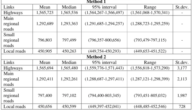
In order to summarize the results, the link flows were aggregated according to the type 15
of road they correspond, the link flow estimates are presented in Table 1. According to the 16
rounded estimates of Table 1, centrality measures, i.e. the means and the medians, derived 17
from the two methods are relatively close, since the differences can be measured in terms of 18
hundreds relative to the large magnitudes of the estimates. This is not the case, for the 95% 19
interval and range estimates, where the estimates of method 2 are much wider than the 20
corresponding estimates of method 1. This is to be expected; as described in section 3.1, 21
percentile estimates from method 1 are approximate since they are derived conditional on the 22
sum of each OD vector, and therefore result to smaller intervals which underestimate the 23
overall input-uncertainty. Method 2, additionally delivers standard deviation estimates which 24
are also included in Table 1. 25
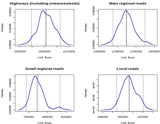
The link flow distributions can be estimated directly from the 200 link flow vectors 26
obtained from method 2; kernel estimates for flows in highways, main regional roads, small 27
regional roads and local roads are presented in Figure 2. Gaussian kernels were used as 28
smoothing kernels, with bandwidths set equal to the corresponding standard deviations of the 29
smoothing kernels. 30
TABLE 1 Mean, Median, 95% Interval (2.5%-97.5%), Range and Standard Deviation Estimates
1
from the 2 Methods for the 4 Types of Link Traffic Flows
2
Method 1
Links Mean Median 95% interval Range St.dev.
Highways 1,565,723 1,565,536 (1,564,267-1,566,497) (1,561,068-1,570,341) - Main regional roads 1,292,689 1,293,363 (1,291,685-1,294,257) (1,288,723-1,295,259) - Small regional roads 796,803 797,499 (796,357-800,656) (793,479-797,115) - Local roads 450,905 450,263 (449,754-450,293) (449,653-451,522) - Method 2
Links Mean Median 95% interval Range St.dev.
Highways 1,565,694 1,565,480 (1,559,776-1,571,443) (1,556,818-1,573,290) 3,177 Main regional roads 1,292,411 1,292,261 (1,288,687-1,297,411) (1,287,121-1,298,399) 2,113 Small regional roads 797,400 797,102 (794,400-803,345) (793,451-805,032) 1,987 Local roads 450,656 450,599 (449,397-452,041) (448,485-452,546) 728 3
A useful application from method 2 is the identification of critical links. Critical link 4
identification is commonly a subject of vulnerability analysis, where state-of-the-art 5
approaches are based on full network scan algorithms ((27), (28)). Nevertheless, the associated 6
computational burden constitutes the implementation of such approaches prohibitive, as yet, 7
for applications on large-scale, congested networks where execution of traffic assignment 8
within the full scan algorithm is additionally required. From this point of view, method 2 9
provides a workable alternative for identifying critical links explicitly in terms of probability. 10
As critical links we define those links in which the V/C ratio exceeds a specific 11
threshold value c with a certain probability, i.e. P(V/ Cc). Evaluation of critical links in 12
terms of probability estimates is safer in comparison to point estimates and also reduces the 13
margin of uncertainty. For instance, the expected value of V/C may be smaller than c , 14
nevertheless the probability of exceeding c may be significantly greater than zero. This point 15
is illustrated further in the proceeding analysis. In general, the value c is the common 1 16
option, since values greater than 1 imply that the traffic flow exceeds the theoretical capacity of 17
a link, thus resulting in congestion. In our case though, inference is limited in traffic flows for 18
work and school trips made only by Flemish residents, which means that we would expect the 19
V/C ratios to be higher if the proportion of traffic related to other trip-purposes and to non-20
Flemish residents was included in the analysis. From this perspective threshold values smaller 21
than 1 may also be regarded as critical, but since the exact proportion of trips which is 22
unaccounted for is not known exactly, c can only be selected on a heuristic basis. As a 23
conservative choice and in order not to overestimate the number of critical links the value of 24
0.95 is adopted. Eleven links are identified as critical for c 0.95, the V/C distributions of 25
these links with the corresponding expected values of V/C ratio and the probabilities of 26
exceeding 0.95 are presented in Figure 3.Note that if the analysis was based on the expected 27
V/C ratio instead of the probability of exceeding a V/C ratio of 0.95, then four out of the eleven 1
links would not have been identified as critical. 2 3 1555000 1565000 1575000 0 .0 0 0 0 0 0 .0 0 0 0 6 0 .0 0 0 1 2
Highways (including entrances/exits)
Link flows D e n s it y 1285000 1290000 1295000 1300000 0 .0 0 0 0 0 0 .0 0 0 1 0 0 .0 0 0 2 0
Main regional roads
Link flows D e n s it y 795000 800000 805000 0 .0 0 0 0 0 0 .0 0 0 1 0 0 .0 0 0 2 0
Small regional roads
Link flows D e n s it y 448000 450000 452000 0 e + 0 0 2 e -0 4 4 e -0 4 Local roads Link flows D e n s it y 4
FIGURE 2 Kernel distributions from method 2 for traffic flows on highways, main regional
5
roads, small regional roads and local roads. The solid, dotted and dashed vertical lines
6
correspond to the mean, median and 95% interval of each distribution, respectively.
7 8
It is interesting to note that the V/C distributions of Figure 3 and consequently the 9
corresponding link flow distributions resulting from DUE assignment are not necessarily close 10
to normal distributions – for instance, bimodality is observed – in contrast to the distributions 11
presented in Figure 2 which are aggregated link flows and in accordance to the central limit 12
theorem closer to normal distributions. 13
Bimodality may be attributed to the iterative user equilibrium procedure itself. For 14
instance, when the flows on a specific link and at a given iteration exceed a certain threshold – 15
consequently leading to a high V/C ratio – and there exists an alternative link which has a cost 16
which is close but lower, then in the following iteration a switch of flows will occur from the 17
high-cost link to the low-cost link. This “switching” effect will eventually result to bimodal 18
V/C distributions, as the ones presented in Figure 3. 19
1
FIGURE 3 V/C kernel distribution estimates from method 2 for the 11 critical links which include
2
or exceed the value of 0.95, highlighted by a vertical line in the distributions which include this
3
value.
4 5
The results in Figure 3 show that seven out of the eleven critical links have a V/C value greater 6
than 0.95 with probability 1. Visual examination of the distributions in Figure 3 additionally 7
reveals that these seven links also exceed the value c with probability 1, except perhaps of 1 8
link 106252 which has its minimum located near 1 and may therefore include smaller values 9
than 1 with a low probability. Conclusively, even without taking into consideration the 10
proportion of traffic related to non-Flemish residents and to other trip-purposes than work or 11
school trips, congestion on these 7 links is almost certain. The highest V/C ratio is observed in 12
highway link 28980 with an expectation of 2.11, while regional road link 16841 and highway 13
link 83928 follow with expected V/C ratios equal to 1.38 and 1.26, respectively. For the 14
remaining 4 links, the probability of exceeding a V/C ratio of 0.95 is lower, equal to 25% for 15
links 83662, 92846 and equal to 3.5% for links 22149 and 29060. Not surprisingly, the 11 16
critical links are situated near the major municipal centers of Antwerp, Ghent and Bruges; the 17
exact locations are presented in Figure 4. 18
As illustrated in Figure 4, five of the critical links belong to the wider municipal area of 19
Antwerp, including link 28980 which is a segment of R1 highway ring in the north of Antwerp 20
and has the highest expected V/C ratio. Links 22149 and 29060 are local outgoing road 21
segments near highway ring R1, whereas link 16841, which has the second highest V/C ratio, 22
is a segment of N1 regional road directing right to the center of Antwerp. Finally, link 17493 is 23
a local road segment outside Antwerp, nevertheless very close to Antwerp airport situated 24
south-east of the city. 25
Five critical links also appear in the municipal area of Ghent. Link 84514 to the north-26
east is a segment of N70 regional road very near the exit of the R4 highway ring with a 27
direction to the center of Ghent, whereas links 83928, 83662, 92486 and 92849, near the 28
center, are all road segments clustered around the end of the part of highway E17 that has a 1
direction to the center of Ghent. 2
Finally, one critical link appears near the municipality of Bruges, that is link 106252. 3
This link corresponds to a local road segment, very near N31 regional road, and with a 4
direction towards the center of Bruges from the west. 5
6
7
FIGURE 4 The critical links in Antwerp, Ghent and Bruges, the link type abbreviations H, MRR,
8
SRR and LR correspond to Highways, Main Regional Roads, Small Regional Roads and Local
9
Roads.
10 11
The analysis of critical links is based on the relatively conservative choice c 0.95. 12
Naturally, for smaller values of c the number of critical links increases, e.g. for the values 0.9, 13
0.85, 0.8, 0.75, 0.7 the number of critical links rises to 16, 20, 25, 47 and 69, respectively. In 14
general, for situations where the exact proportion of traffic is not known, as in the application 15
presented in this study, the choice of c is under the control of the researcher or policy-planner. 1
In such cases, inference may be based on more than one values of c . For cases in which there 2
is certainty that all the potential traffic or – at least – most of the potential traffic of a network 3
is included in the analysis, then the value c may be safely adopted. 1 4
5
5. CONCLUSIONS 6
7
This study focuses on utilizing Bayesian OD predictions as input in traffic assignment models, 8
as a mean of incorporating and quantifying input-uncertainty. Two methods of inputting OD 9
predictions are proposed. In the first method, an OD summary is calculated from the multiple 10
OD predictions and is assigned to the corresponding network. Whereas, in the second method 11
all OD predictions are assigned to the network individually. 12
In terms of computational expense, the first method is less demanding and suitable for 13
delivering basic inferential tools, such as point and approximate interval estimates of link 14
flows, with a limited number of assignments. On the other hand, method 2 results to more 15
reliable interval estimates and also provides dispersion and distributional estimates which are 16
not computable through method 1. 17
In general, method 2 provides greater inferential capabilities and gives rise to novel 18
applications as is the identification of critical links explicitly in terms of probability estimates. 19
The proposed methods can be applied on short-term as well as long-term OD matrices 20
and furthermore their use in not constrained by the selection of the assignment model. 21
Therefore, the methods may be utilized for different travel-demand perspectives under 22
deterministic and stochastic assignment models. 23
An application for the road network of Flanders was presented for the morning peak 24
hour between 7 am and 8 am, under the assumption of a DUE model and by utilizing 200 25
predictive OD matrices. Traffic flows in Flanders were found to be denser around the major 26
municipal centers of Antwerp, Ghent, Leuven and Bruges and on the highways which connect 27
these cities with each other and also with Brussels. Eleven critical links were identified for a 28
threshold value of 0.95, the majority of which belonging to Antwerp and Ghent. 29
Future research will focus further on implementing both methods under system 30
optimum and also deterministic/stochastic user equilibrium assignment assumptions for various 31
travel-demand scenarios. That would allow for a comparison between theoretical expectations 32
and the actual performance of those models, under different experimental settings. 33
REFERENCES 1
2
(1) Cascetta, E. Transportation Systems Analysis: Models and Applications, Second Edition. 3
Springer, New York, 2009. 4
(2) Thomas, R. Traffic Assignment Techniques. Avebury Technical, Aldershot, 1991. 5
(3) Patriksson, M. Traffic Assignment Problems: Models and Methods. Topics in 6
transportation. V.N.U. Science Press, Utrecht, 1994.
7
(4) Florian, M. and D. Hearn. Network equilibrium models and algorithms. In Handbooks in 8
OR and MS, Vol. 8, 1995, pp. 485-550.
9
(5) Cantarella, G. E. and E. Cascetta. Stochastic assignment to transportation networks: 10
models and algorithms. In Equilibrium and advanced transportation modelling, Vol.5, 11
1998, pp. 87–107. 12
(6) de Jong, G., A. Daly, M. Pieters, S. Miller, R. Plasmeijer, and F. Hofman. Uncertainty in 13
traffic forecasts: literature review and new results for The Netherlands. Transportation, 14
Vol. 34, No. 4, 2006, pp. 375-395. 15
(7) Ettema, D. and H. Timmermans. Costs of travel time uncertainty and benefits of travel 16
time information: Conceptual model and numerical examples. Transportation Research 17
Part C: Emerging Technologies, Vol. 14, No. 5, 2006, pp. 335-350.
18
(8) Li, R. and G. Rose. Incorporating uncertainty into short-term travel time predictions. 19
Transportation Research Part C: Emerging Technologies, Vol. 19, No. 6, 2011, pp.
1006-20
1018. 21
(9) Kuhn, K. D. and S. M. Madanat. Model uncertainty and the management of a system of 22
infrastructure facilities. Transportation Research Part C: Emerging Technologies, Vol. 23
13, No. 5-6, 2005, pp. 391-404. 24
(10) Ng, M., Z. Zhang, and S. T. Waller. The price of uncertainty in pavement infrastructure 25
management planning: An integer programming approach. Transportation Research Part 26
C: Emerging Technologies, Vol. 19, No. 6, 2011, pp. 1326-1338.
27
(11) Matas, A., J. L. Raymond, and A. K. Ruiz. Traffic forecasts under uncertainty and 28
capacity constraints. Transportation, in press, doi: 10.1007/s11116 -011-9325-1. 29
(12) Hazelton, M.L. Some remarks on stochastic user equilibrium. Transportation Research 30
Part B: Methodological, Vol. 32, No. 2, 1998, pp. 101-108.
31
(13) Waller, S.T., J. Schofer, and A. Ziliaskopoulos. Evaluation with traffic assignment under 32
demand uncertainty. Transportation Research Record: Journal of the Transportation 33
Research Board, Vol. 1771, No. 1, 2001, pp. 69-74.
34
(14) Ukkusuri, S. V. and S. T. Waller. Single-point approximations for traffic equilibrium 35
problem under uncertain demand. Transportation Research Record: Journal of the 36
Transportation Research Board, Vol. 1964, No. 1, 2006, pp. 169-175.
37
(15) Gardner, L. M., A. Unnikrishnan, and S. Waller. Robust pricing of transportation 38
networks under uncertain demand. Transportation Research Record: Journal of the 39
Transportation Research Board, Vol. 2085, No. 1, 2008, pp. 21-30.
40
(16) Gardner, L. M., A. Unnikrishnan, and S. T. Waller. Solution methods for robust pricing of 41
transportation networks under uncertain demand. Transportation Research Part C: 42
Emerging Technologies, Vol. 18, No. 5, 2010, pp. 656-667.
43
(17) Duthie, J. C., A. Unnikrishnan, and S. T. Waller. Influence of demand uncertainty and 44
correlations on traffic predictions and decisions. Computer Aided Civil and Infrastructure 45
Engineering, Vol. 26, No. 1, 2011, pp. 16-29.
(18) Ukkusuri, S. V., T. V. Mathew, and S. T. Waller. Robust transportation network design 1
under demand uncertainty. Computer Aided Civil and Infrastructure Engineering, Vol. 2
22, No. 1, 2007, pp. 6-18. 3
(19) Ukkusuri S. V. and G. Patil. Multi-period transportation network design under demand 4
uncertainty. Transportation Research Part B: Methodological, Vol. 43, No. 6, 2009, pp. 5
625-642. 6
(20) Perrakis, K., D. Karlis, M. Cools, D. Janssens, K. Vanhoof, and G. Wets. A Bayesian 7
approach for modeling origin-destination matrices. Transportation Research Part A: 8
Policy and Practice, Vol. 46, No. 1, 2012, pp. 200-212.
9
(21) Fernández, C., E. Ley, and M. F. J. Steel. Benchmark priors for Bayesian model 10
averaging. Journal of Econometrics, Vol. 100, No. 2, 2001, pp. 381-427. 11
(22) Ntzoufras, I. Bayesian Modeling Using WinBUGS. John Wiley and Sons, Inc., Hoboken, 12
New Jersey, 2009. 13
(23) Gamerman, D. and H.F. Lopes. Markov Chain Monte Carlo: Stochastic Simulation for 14
Bayesian Inference, Second Edition. Chapman and Hall/CRC, London, 2006.
15
(24) Hastings, W. K. Monte Carlo sampling methods using Markov chains and their 16
applications. Biometrika, Vol. 57, No. 1, 1970, pp. 97-109. 17
(25) Agresti, A. Categorical Data Analysis, Second edition. John Wiley and Sons, Inc., 18
Hoboken, New Jersey, 2002. 19
(26) Bureau of Public Roads. Traffic assignment manual for application with a large, high 20
speed computer. U.S. Department of Commerce, 1964.
21
(27) Jenelius, E., T. Petersen, and L.G. Mattsson. Importance and exposure in road network 22
vulnerability analysis. Transportation Research Part A: Policy and Practice, Vol. 40, No. 23
7, 2006, pp. 537-560. 24
(28) Taylor, M. A. P. Critical transport infrastructure in urban areas: impacts of traffic 25
incidents assessed using accessibility-based network vulnerability analysis. Growth and 26
Change, Vol. 39, No. 4, 2008, pp. 593-616.