A relaxation scheme to combine Phasor-Mode and
Electromagnetic Transients Simulations
Frédéric J. Plumier
a [email protected]Petros Aristidou
a [email protected]Christophe Geuzaine
a [email protected]Thierry Van Cutsem
b [email protected]Abstract—This paper deals with a new scheme for coupling phasor-mode and electromagnetic transients simulations. In each simulation, an iteratively updated linear equivalent is used to represent the effect of the subsystem treated by the other simulation. Time interpolation and phasor extraction methods adapted to this scheme are presented and compared to existing methods. Finally, simulation results obtained with a 74-bus test system are reported.
Index Terms—hybrid simulations, multirate techniques, phasor approximation, electromagnetic transients, boundary conditions.
I. INTRODUCTION A. Overall objective of the work
C
OUPLED simulations of power systems, combining Phasor-Mode (PM) and ElectroMagnetic Transients (EMT) models, aim at taking advantage of the high speed of PM simulations and the high accuracy of EMT simulations. To this purpose, the EMT model is simulated with a “small” time step size h and the PM model with a “large” time step size H. This feature makes the combined PM-EMT simulation a particular case of multirate methods. A typical example of application is the detailed simulation of an unbalanced fault using the EMT model in a subsystem surrounding the fault location, and the PM model for the rest of the power system. The first related work can be traced back to 1981 [1]. Since then, a significant number of advances have taken place, as testified by the state-of-the-art report in [2]. However, there is still room for improvement in coupled PM-EMT simulations, to reach the targeted speed-accuracy compromise. Some authors even challenge the theoretical basis supporting this type of hybrid simulation [3].This paper revisits and improves the techniques to represent one subsystem into the simulation of the other, and extract the relevant signals from one simulation, for use in the other.
B. Simplified representation of EMT and PM subsystems
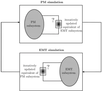
Figure 1 illustrates two issues addressed in this paper. First, the coupling of PM and EMT simulations implies modelling the PM subsystem’s response when performing the EMT simulation, and conversely. This requires choosing a simplified representation of the EMT subsystem, to be used in PM simulation, and a simplified representation of the
aDept. of Elec. Eng. and Comp. Science, University of Liège, Belgium. bFNRS at Dept. of Elec. Eng. and Comp. Science, University of Liège, Belgium.
Figure 1. Overall scheme of coupled phasor-mode and electromagnetic transients simulations
PM subsystem, for use in the EMT simulation. Second, this work considers the possibility to iterate between both models, at each discrete time of the simulation, until satisfactory convergence is reached and simulation proceeds with the next discrete time. The choice of the simplified representations of, respectively, the EMT and the PM subsystem impacts the speed of convergence of this relaxation process.
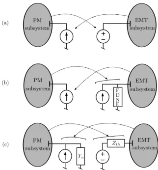
For the sake of simplicity, this paper focuses on the case where the PM and EMT subsystems are connected to each other through a single boundary bus. Three simple models come to mind for the representation of either of the two systems, when simulating the other: (i) an ideal voltage source attached to the boundary bus; (ii) an ideal current source injecting into the boundary bus, or (iii) a linear relation between the boundary voltage and current, in the form of a Thévenin (or Norton) equivalent.
Figure 2 summarizes the combinations of representations documented in the literature.
In Ref. [4], it was chosen to use an ideal current source to represent the EMT subsystem in the PM model, and an ideal voltage source to represent the PM subsystem in the EMT model, as shown in Fig. 2.a. While this configuration offers the advantage of simplicity, it requires to have, at the boundary, three-phase voltages and currents with negligible imbalance
Figure 2. Simplified representations of the PM and EMT subsystems at the boundary bus
and distortion since this is the usual assumption taken in phasor-mode simulation. In turn, this requires to place the boundary far enough from the location of the disturbance, i.e. to have a large enough EMT subsystem. With the increasing computational power available nowadays, it should generally not be a problem to increase the size of the EMT subsystem until fundamental-frequency positive-sequence currents are observed at the boundary with the PM subsystem.
The approach used in [5] is shown in Fig. 2.b. While still relying on a current source to represent the EMT subsystem, it uses a Frequency Dependent Network Equivalent (FDNE) admittance in parallel with an ideal current source to represent the PM subsystem. This more accurate representation, valid over a wide frequency range, allows putting the boundary closer to the disturbance location without degrading accuracy. The representation considered in this paper resorts to the use of both a Norton and a Thévenin equivalent, as shown in Fig. 2.c. Note that choosing between a Norton or a Thévenin representation is free; the shown combination is convenient for incorporation in the usual PM and EMT models. Apparently, this approach can be traced back to Ref. [6] but, to the authors’ knowledge, it has not been used in any recent, published work. The reason may be that researchers oriented their efforts towards improving the representation of the PM subsystem in the EMT simulation in order for the boundary to be located closer to the disturbance without losing accuracy.
It must be emphasized that the impedance, admittance, voltage and current parameters involved in the equivalents are updated during the dynamic simulation, while iterating between the PM and EMT simulations. Thus, the method differs from merely using a fixed Thévenin or Norton equiva-lent to represent the other subsystem. More details about this
Extraction PM simulation EMT simulation Time Interpolation Phasor
Figure 3. Time interpolation and phasor extraction steps
relaxation procedure are given in Section II.
C. Information exchanged by PM and EMT simulations
The EMT and PM simulations must receive information compatible with their modelling assumptions. This requires performing time interpolation and phasor extraction, respec-tively, as shown in Fig. 3.
Time interpolation is needed to convert the “slowly” varying voltage and current phasors, provided by the PM simulation, into voltage and current sources evolving sinusoidally with time, at the nominal fundamental frequency, but with “slowly varying” magnitudes and phase angles. While a simple linear time interpolation can be used for that purpose, there are some problematic situations, such as the application of a fault close to the boundary between the EMT and PM subsystems. This and other issues are addressed in Section III.
Phasor extraction, used for passing information from EMT to PM simulation, consists in extracting the positive-sequence phasors from three-phase, possibly distorted and unbalanced, bus voltage and branch current signals sampled at period h. In the context of hybrid simulations, a phasor extraction method was early proposed in [1], using RMS approximations to obtain power and a Fast Fourier Transform (FFT) to determine the fundamental voltage magnitude. The drawback of FFT and similar approaches is that they introduce a time delay. An improved method has been proposed in [7], relying on instantaneous values of real and reactive power. This method resorts to energy balance to extract the current phasor.
In contrast, the method detailed in Section IV, which ex-tends the one proposed in [4], resorts to projections on rotating axes to extract voltage or current phasors. To the best of the authors’ knowledge, this procedure has not been considered elsewhere, which might explain why the representation shown in Fig. 2.c has not been used either.
II. RELAXATION PROCESS BETWEENEMTANDPM
SIMULATIONS
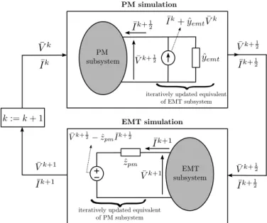
The relaxation scheme sketched in Fig. 1 is shown in greater detail in Fig. 4. The two simulations exchange phasors. This assumes that the boundary is far enough from the disturbance, so that phase imbalances, aperiodic components and harmonics can be neglected, as discussed in the Introduction.
The focus is on iterations performed when passing from time t to time t + H, i.e. over one step of the PM simulation. At the k-th iteration, given the estimates ( ¯Vk, ¯Ik) of the
Figure 4. Relaxation process with iteratively updated equivalents to account for one subsystem when simulating the other subsystem
simulation determines the evolution of the PM subsystem over a single step H, with the EMT subsystem replaced by a Norton equivalent. The latter involves an admittance ˆyemt and the
Norton current: ¯
Ino= ¯Ik+ ˆyemtV¯k (1)
updated with the latest available boundary voltage and current. The PM simulation yields the new estimates ( ¯Vk+1
2, ¯Ik+12) of
the boundary voltage and current, where the upperscript k +12 indicates that half of the iteration has been performed.
In case a fault is simulated (taking place in the EMT subsystem), ˆyemt can be computed beforehand for the
pre-fault, during-fault and post-fault situations. Alternatively, it could be estimated numerically, from the previous values of the boundary voltage and current.
Given the updated values ( ¯Vk+1
2, ¯Ik+12) of the boundary voltage and current phasors at time t+H, the EMT simulation provides the evolution of the EMT subsystem from t to t + H, using small time steps h with the PM subsystem replaced by a Thévenin equivalent. The latter involves an impedance ˆ
zpm (also determined beforehand or estimated during the
iterations), and the Thévenin voltage: ¯ Eth= ¯Vk+ 1 2 − ˆzpmI¯k+ 1 2 (2)
updated with the latest available boundary voltage and current. In the EMT simulation, this Thévenin equivalent is replaced by differential equations as the rest of the EMT model. This simulation yields the new estimates ( ¯Vk+1, ¯Ik+1).
Convergence is checked by comparing|| ¯Vk+1− ¯Vk|| and
||¯Ik+1− ¯Ik|| to some tolerances. If the latter are satisfied, the
simulation proceeds with the next time interval [t+H t+2H]. Otherwise, an additional relaxation iteration is performed.
Let ¯Vpmand ¯Ipm(resp. ¯Vemtand ¯Iemt) be the values of the
boundary voltage and current, provided by PM (resp. EMT)
Figure 5. Situation reached when the relaxation process has converged
simulation, once convergence has taken place. At convergence, the circuits in Fig. 4 operate as shown in Fig. 5, where intermediate values have been replaced by final ones.
The following equations are easily derived from Fig. 5: ¯
Ipm = I¯emt+ ˆyemtV¯emt− ˆyemtV¯pm (3)
¯
Vemt = V¯pm− ˆzpmI¯pm+ ˆzpmI¯emt (4)
Introducing (4) into (3) and rearranging the terms yields: (1+ˆzpmyˆemt) ¯Ipm= (1+ˆzpmyˆemt) ¯Iemt ⇔ ¯Ipm= ¯Iemt (5)
where it has been assumed that the parenthesis is nonzero. Hence, Eq. (3) becomes:
¯
Vpm= ¯Vemt (6)
From Eqs. (5) and (6) it is concluded that, whatever the values
of ˆyemt and ˆzpm, the converged solution reached by the PM
and EMT simulations is such that the boundary bus has the same voltage in both of them, and the current injected by one is the current received by the other. Thus, there is a perfect match between the PM and EMT simulations. On the other hand, the values of ˆyemt and ˆzpm influence the convergence
of the relaxation process. For instance, if ˆyemtwas set to zero,
at the k-th iteration the PM simulation would be performed with the boundary current set to ¯Ik; hence, the current change
induced by the change of voltage ¯Vk would be accounted for
at the (k + 1)-th iteration only. The Norton equivalent (with ˆ
yemt ̸= 0) yields a linear approximation of that variation of
the current with the voltage. Similar considerations apply to the Thévenin equivalent and ˆzpm.
One can reasonably assume that, the more accurate the linear approximation, the faster the convergence of the re-laxation process. This assertion is supported by numerical results in [8], where the rate of convergence of the relaxation scheme is assessed under the assumption that the EMT and PM subsystem behave linearly.
The PM and EMT simulations match for any choice of ˆyemt
and ˆzpm, provided the PM and EMT models are iterated until
convergence. The same does not hold true if a single iteration is performed, i.e. a single PM simulation followed by a single EMT simulation when passing from t to t + H. This case is of interest when hybrid simulation is used to test “hardware in the loop” [9]. In that application, ˆyemt and ˆzpm should be
Figure 6. Interpolating the Thévenin voltage phasor
III. FROMPMTOEMT: TIME INTERPOLATION
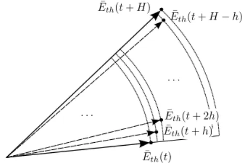
Consider an EMT simulation over the time interval [t t+H]. Thus, the values of all states at time t have been computed and accepted; the ones at time t + H are being computed. The last PM simulation provides the estimates ¯Vk+1
2(t + H) and ¯
Ik+1
2(t + H) of the boundary voltage and current (see Fig. 4). The corresponding estimated Thévenin voltage is given by:
¯ Eth(t + H) = ¯Vk+ 1 2(t + H)− ˆzpmI¯k+ 1 2(t + H) (7) A linear interpolation of respectively the magnitude and the phase angle of ¯Eth is considered, as shown in Fig. 6. For
simplicity of presentation, H is assumed to be a multiple of
h, i.e. H = ρh where ρ is an integer. Thus, at the discrete
time t + nh (n = 0, . . . , ρ), the interpolated Thévenin voltage magnitude is given by:
E(t+nh) =|| ¯Eth(t)||+ n ρ ( || ¯Eth(t + H)|| − || ¯Eth(t)|| ) (8) where|| || denotes the magnitude. The interpolated phase angle is given by:
ϕ(t + nh) =∠Eth(t) +
n
ρ(∠Eth(t + H)− ∠Eth(t)) (9)
Considering phase a, for instance, the discretized Thévenin voltage is obtained as (n = 0, . . . , ρ):
ea(t+nh) =
√
2E(t+nh) sin (ω(t + nh) + ϕ(t + nh)) (10) where ω is the nominal angular speed of the system.
The simulation of large disturbances, typically faults, in the EMT subsystem calls for some comments. In such a case, the phasor of the voltage at the boundary is expected to undergo a fast and significant change (although this is attenuated by setting the boundary with the PM subsystem far enough the fault location). An example is provided in Fig. 7 showing the evolution of a boundary bus voltage in response to a three-cycle fault applied at t = 20 ms and cleared at t = 80 ms.
There are two issues: accuracy and convergence of the relaxation process.
For what concerns accuracy, the use of a Thévenin equiva-lent reproduces the sharp voltage drop in the EMT simulation. As regards convergence, the advantage of approximating the response of the PM subsystem by a Thévenin equivalent is worth being repeated. By so doing, the abrupt change in volt-age is already rendered by the first EMT simulation, through
-2 -1 0 1 2 0 20 40 60 80 100 120 V (pu) t (ms) PM EMT phase a b c
Figure 7. Example of evolution of voltage at boundary bus during a fault
the voltage drop in the Thévenin impedance ˆzpm. This feature
would not be obtained with a pure voltage source as shown in Fig. 2.a (upper right diagram). The problem was reported in [10], where it is suggested to use the voltage ¯Vk+1
2(t + H) over the whole time interval H instead of interpolation. On the contrary, the use of a Thévenin equivalent preserves the convergence of the relaxation process. For instance, in the case of Fig. 7, it was possible to use steps of 20 ms in the PM simulation, as shown by the curve labelled “PM” in the figure.
IV. FROMEMTTOPM: PHASOR EXTRACTION
As shown in Fig. 4, the EMT simulation provides updated estimates(V¯k+1, ¯Ik+1)of the boundary voltage and current.
The positive-sequence phasor of either the current or the voltage is extracted. Assuming arbitrarily that it is the current, the boundary voltage phasor is easily obtained from Fig. 4 as:
¯
Vk+1= ¯Vk+12 + ˆzpm( ¯Ik+1− ¯Ik+ 1
2) (11)
The phasor extraction consists of two steps: (i) projection on a rotating reference frame, using the method initially proposed in [4], and (ii) post-processing using a low-pass filter, which improves that method.
A. Projection on a rotating reference frame
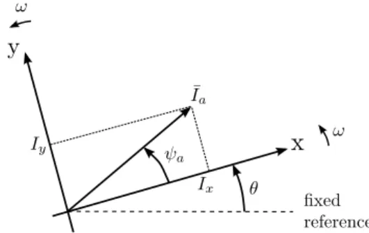
The amplitude and the phase angle of the positive-sequence component of the currents are computed from the three time-varying current waveforms by projecting the latter on (x, y) reference axes, using a Park-type transform. This technique, inspired of the principle of Phase Locked Loop (PLL) systems [11], is free from any delay associated with processing of the current waveforms.
More precisely, (x, y) are the orthogonal axes used in the PM simulation to project the rotating vectors associated with quasi-sinusoidal variables, and obtain their corresponding rectangular components. As shown in Fig. 8, these axes rotate at the nominal angular speed ω and, at time t, the x axis is at an angular position:
Figure 8. reference axes and phasors involved in the extraction of the positive-sequence component of the boundary current
with respect to a fixed reference, where the position of the
x-axis at t = 0 has been arbitrarily set to zero.
The current waveforms to process can be written as:
iabc= iiab ic = √ 2Iacos (ωt + ψa) + ϵa √ 2Iacos ( ωt + ψa−2π3 ) + ϵb √ 2Iacos ( ωt + ψa−4π3 ) + ϵc (13) where ϵa, ϵb and ϵc are noise terms accounting for
devia-tions with respect to three-phase, balanced, positive-sequence components. The current in iabc are projected on the above
mentioned axes by applying the linear transform [12]: i0xy= Tiabc (14) with: T = √ 2 3 1/√2 1/√2 1/√2
cos (θ) cos(θ−2π3) cos(θ−4π3) − sin (θ) − sin(θ−2π3) − sin(θ−4π3)
(15) In the ideal case where the three currents make up a balanced, positive sequence, i.e. ϵa = ϵb = ϵc = 0, the
projected currents are easily obtained as:
i0xy= ii0x iy = Iacos ψ0 a Iasin ψa (16)
The last two components are the projections on x and y of a vector rotating at angular speed ω, representing the current in phase a, having an amplitude Ia and a phase angle ψa with
respect to the x axis (see Fig. 8). In the PM simulation, ix
and iy are the rectangular components of the current source
shown in the upper block of Fig. 4. Its magnitude and phase angle are easily obtained as:
Ia= √ i2 x+ i2y ψa= arctan ( iy ix ) (17) At this point of the procedure, Eq. (14) is applied only to the currents iabcobtained at time t+H of the EMT simulation.
B. Low-pass filtering
Because the effects of a fault located in the EMT subsystem are expected to be still felt at the boundary between PM and EMT subsystems, the boundary current waveforms contain
noise terms. The latter stem from aperiodic, negative- and zero-sequence components, and harmonics, whose effect must be filtered out.
While three-phase, balanced, positive-sequence currents are converted into constant ix and iy, aperiodic (resp.
negative-sequence) components present in the phase currents will be transformed into sinusoidal components at nominal (resp. double nominal) frequency. Thus, the filter must:
• preserve the amplitude of components with frequencies between 0 and 5 Hz. This covers the frequency spectrum of concern in PM simulation;
• filter out the fundamental-frequency, double-fundamental-frequency and higher frequency components;
• not affect the phase of the initial signal in the [0 5] Hz frequency range, to avoid introducing any delay between the EMT and PM simulations.
This low-pass numerical filter processes sampled ix and iy
values obtained by applying (14) at equidistant discrete times in [t t + H]. The sampling period can be h, the time step size used in EMT simulation. Re-sampling may be necessary in case the discrete times of the EMT simulation are not equidistant, for instance because it was necessary to reduce the time step size during the simulation. The width H of the time interval processed by the filter is usually no smaller than one half cycle at the nominal frequency, and most often closer to one cycle. It may be occasionally reduced, for instance at fault application and clearing. The time interval processed by the filter should not become too narrow, for accuracy reasons. Satisfactory results have been obtained with a Butterworth low-pass filter. For a continuous-time filter, the magnitude-squared transfer function takes on the form:
∥Hc(jω)∥
2
= 1
1 + (jω/jωc)
2N (18)
where ωc is the cutoff frequency. This filter is characterized
by a magnitude response maximally flat in the passband. This means that the first 2N − 1 derivatives of the function (18) are zero at ω = 0 [13].
The filter is applied twice, once with increasing and once with decreasing times. Doing so should almost cancel the phase shift introduced by the filter in the pass-band. The order of the filter has been taken to two. However, applying the filter twice yields globally a fourth-order filter, which is expected to give sufficient cut-off band attenuation for most systems.
V. SIMULATION RESULTS A. Test system and computing tools
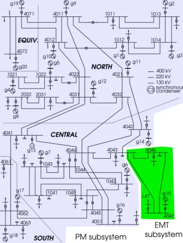
Tests have been performed on the 74-bus, 102-branch, 20-machine Nordic test system documented in [14] and shown in Fig. 9. The RAMSES software developed at the University of Liège [15] has been used for PM simulation, while the EMT subsystem solver was implemented in MATLAB, communi-cating with RAMSES. The results of the PM-EMT simulation have been compared to those given by EMTP-RV applied to
subsystem PM subsystem EMT g20 g17 g18 g2 g11 g16 g19 g9 g1 g3 g13 g8 g12 g4 g5 g10 g7 g15 L47 g14 g6 4011 4012 1011 1012 1014 1013 1022 1021 2031 cs 4046 4043 4044 4032 4031 4022 4021 4071 4072 4041 1042 1045 1041 4063 4061 1043 1044 4047 4051 4045 4062 400 kV 220 kV 130 kV synchronous condenser CS NORTH CENTRAL EQUIV. SOUTH 4042 2032
Figure 9. Nordic test system decomposed into PM and EMT subsystems
the whole system. The trapezoidal rule was used with a step size h of 50 µs, and a step size H of 20 ms.
This paper reports on preliminary tests in which only a small EMT subsystem has been considered. It is identified in Fig. 9. It includes six buses, two loads and one synchronous machine represented in detail. It is connected to the rest of the system through a single interface bus (4043).
B. Case 1: tripping the three-phase load L47
The 100 MW/44 MVar load connected to bus 47 is tripped at t = 1 s. Figure 10 shows the evolution of the voltage magnitude at the boundary bus, given by the proposed method and EMTP-RV, respectively. There is a reasonably good match between both responses.
Figure 11 shows that the same hold true for the rotor speed of machine g15, located in the EMT subsystem. The response shows the effect of speed governors, installed on generators in the NORTH and EQUIV areas, i.e. in the PM subsystem.
Further tests involve comparing the response of components located in the PM subsystem. An example is provided by Fig. 12, showing the rotor speed of g14, located very near the boundary bus. Incidentally, this figure illustrates the ad-vantage of hybrid simulation with respect to replacing the PM subsystem by a simple equivalent. The former, by preserving the topology of the system, not only offers more accuracy
1.036 1.04 1.044 0 5 10 15 20 V (pu) t (s) emtp-rv PM-EMT 1.044 7 15
Figure 10. Case 1. Boundary bus voltage magnitude
1 1.0002 1.0004 1.0006 1.0008 0 5 10 15 20 omega (pu) t (s) emtp-rv PM-EMT
Figure 11. Case 1. Speed of machine g15
1 1.0002 1.0004 1.0006 1.0008 0 5 10 15 20 omega (pu) t (s) emtp-rv PM-EMT
Figure 12. Case 1. Speed of machine g14
but also gives access to individual components for which the phasor approximation is valid.
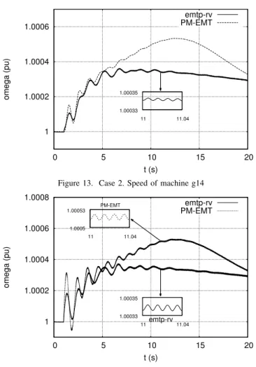
C. Case 2: tripping one phase of load L47
This case involves an unbalanced disturbance in the EMT subsystem, namely the opening of one phase of the load L47. Figure 13 shows the evolution of the rotor speed of g14. As expected, the EMTP-RV simulation reveals the presence of negative-sequence 100-Hz oscillations. The latter are not rendered by the PM-EMT simulation since g14 is located in the PM subsystem, where only the positive sequence is
1 1.0002 1.0004 1.0006 0 5 10 15 20 omega (pu) t (s) emtp-rv PM-EMT 1.00033 1.00035 11 11.04
Figure 13. Case 2. Speed of machine g14
1 1.0002 1.0004 1.0006 1.0008 0 5 10 15 20 omega (pu) t (s) PM-EMT emtp-rv emtp-rv PM-EMT 1.00033 1.00035 11 11.04 1.0005 1.00053 11 11.04
Figure 14. Case 2. Speed of machine g15
considered. On the other hand, Fig. 14 shows that these oscillations are present in both simulations for g15, located in EMT subsystem.
In this case the responses provided by the EMTP-RV and PM-EMT simulations are in less good agreement. This is due to the boundary (bus 4043) being too close to the disturbance location (bus 47), which causes the boundary phase currents to include other than positive-sequence components. For more accurate results, the EMT subsystem should be somewhat enlarged.
VI. CONCLUSION
In this paper, a hybrid simulation combining PM and EMT models has been proposed. The heart of the method is a relaxation process between one “large” time step of the PM simulation and multiple “small” time steps of the EMT simulation.
A key point of this process is the inclusion of iteratively updated Thévenin/Norton equivalents to account for one sub-system when simulating the other subsub-system. It has been shown that, whatever the values of the Thévenin impedance or Norton admittance, at convergence, there is a perfect match between both simulations. On the other hand, these parameters impact the convergence of the relaxation process.
The Thévenin voltage passed by the PM to the EMT simulation is linearly interpolated over the small time steps
of the EMT simulation. Conversely, boundary voltage and current phasors are extracted from the waveforms of the EMT simulation, and passed to the PM simulation. The phasor extraction involves a projection on a rotating reference frame followed by a low-pass filtering.
The method has been illustrated through a sample of re-sults obtained with a 74-bus system including a 6-bus EMT subsystem. A reasonably good match has been found between the proposed method and a full EMPT-RV simulation. More accurate results are expected by slightly enlarging the EMT subsystem, so that the boundary currents better satisfy the positive-sequence assumption underlying the PM simulation.
ACKNOWLEDGMENT
Work supported by the Belgian Science Policy (IAP P7/02) and by Walloon Region of Belgium (WBGreen Grant FEDO).
REFERENCES
[1] M. Heffernan, K. Turner, J. Arrillaga, and C. Arnold, “Computation of AC-DC system disturbances - Part I, II and III. interactive coordination of generator and converter transient models,” IEEE Transactions on
Power Apparatus and Systems, vol. 100, no. 11, pp. 4341 – 4363, 1981.
[2] V. Jalili-Marandi, V. Dinavahi, K. Strunz, J. Martinez, and A. Ramirez, “Interfacing techniques for transient stability and electromagnetic tran-sient programs,” IEEE Transactions on Power Delivery, vol. 24, no. 4, pp. 2385 – 2395, 2009.
[3] S. Fan and H. Ding, “Time domain transformation method for acceler-ating EMTP simulation of power system dynamics,” IEEE Transactions
on Power Systems, vol. 27, pp. 1778–1787, 2012.
[4] F. Plumier, C. Geuzaine, and T. Van Cutsem, “A multirate approach to combine electromagnetic transients and fundamental-frequency sim-ulations,” in Proceedings of International Conference on Power System
Transients (IPST), 2013.
[5] Y. Zhang, A. Gole, W. Wu, B. Zhang, and H. Sun, “Development and analysis of applicability of a hybrid transient simulation platform combining TSA and EMT elements,” IEEE Transactions on Power
Systems, vol. 28, no. 1, pp. 357–366, 2013.
[6] G. W. Anderson, “Hybrid simulation of AC-DC power systems,” Ph.D. dissertation, University of Canterbury, Christchurch, New Zealand, 1995. [7] X. Lin, A. Gole, and M. Yu, “A wide-band multi-port system equivalent for real-time digital power system simulators,” IEEE Transactions on
Power Systems, vol. 24, no. 1, pp. 237–249, 2009.
[8] F. J. Plumier, C. Geuzaine, and T. Van Cutsem, “On the convergence of relaxation schemes to couple phasor-mode and electromagnetic transients simulations,” paper accepted for presentation at the IEEE PES General Meeting, Washington DC, July 2014. [Online]. Available: http://hdl.handle.net/2268/163099
[9] K. P. P. J. Mosterman, Ed., Real-Time Simulation Technologies:
Princi-ples, Methodologies, and Applications. CRC Press, 2013.
[10] S. Abhyankar and A. Flueck, “An implicitly-coupled solution approach for combined electromechanical and electromagnetic transients simula-tion,” in Power and Energy Society General Meeting, 2012 IEEE, july 2012, pp. 1 –8.
[11] S.-K. Chung, “A phase tracking system for three phase utility interface inverters,” IEEE Transactions on Power Electronics, vol. 15, no. 3, pp. 431 –438, may 2000.
[12] G. Paap, “Symmetrical components in the time domain and their application to power network calculations,” IEEE Transactions on Power
Systems, vol. 15, no. 2, pp. 522 –528, may 2000.
[13] A. V. Oppenheim and R. W. Schafer, Discrete-time signal processing. Prentice-Hall, 1989.
[14] T. Van Cutsem and L. Papangelis, “Description, modeling and simulation results of a test system for voltage stability analysis,” University of Liège, Internal report, 2013. [Online]. Available: http://hdl.handle.net/2268/141234
[15] D. Fabozzi, B. Haut, A. Chieh, and T. Van Cutsem, “Accelerated and localized Newton schemes for faster dynamic simulation of large power systems,” IEEE Transactions on Power Systems, vol. 28, no. 4, pp. 4936– 4947, 2013. [Online]. Available: http://hdl.handle.net/2268/144154