Astronomy & Astrophysics manuscript no. BinaryRossiterI˙v4 ESO 2012c August 27, 2012
The EBLM Project
?
I – Physical and orbital parameters, including spin–orbit angles, of two low-mass
eclipsing binaries on opposite sides of the Brown Dwarf limit
Amaury H.M.J. Triaud
1, Leslie Hebb
2, David R. Anderson
3, Phill Cargile
2, Andrew Collier Cameron
4, Amanda P.
Doyle
3, Francesca Faedi
5, Micha¨el Gillon
6, Yilen Gomez Maqueo Chew
5, Coel Hellier
3, Emmanuel Jehin
6, Pierre
Maxted
3, Dominique Naef
1, Francesco Pepe
1, Don Pollacco
5, Didier Queloz
1, Damien S´egransan
1, Barry Smalley
3,
Keivan Stassun
2, St´ephane Udry
1, and Richard G. West
71 Observatoire Astronomique de l’Universit´e de Gen`eve, Chemin des Maillettes 51, CH-1290 Sauverny, Switzerland 2 Department of Physics and Astronomy, Vanderbilt University, Nashville, TN37235, USA
3 Astrophysics Group, Keele University, Staffordshire, ST55BG, UK
4 SUPA, School of Physics & Astronomy, University of St Andrews, North Haugh, KY16 9SS, St Andrews, Fife, Scotland, UK 5 Astrophysics Research Centre, School of Mathematics & Physics, Queens University, University Road, Belfast, BT71NN, UK 6 Institut d’Astrophysique et de G´eophysique, Universit´e de Li`ege, All´ee du 6 Aoˆut, 17, Bat. B5C, Li`ege 1, Belgium
7 Department of Physics and Astronomy, University of Leicester, Leicester, LE17RH, UK
Received date/ accepted date
ABSTRACT
This paper introduces a series of papers aiming to study the dozens of low mass eclipsing binaries (EBLM), with F, G, K primaries, that have been discovered in the course of the WASP survey. Our objects are mostly single-line binaries whose eclipses have been detected by WASP and were initially followed up as potential planetary transit candidates. These have bright primaries, which facilitates spectroscopic observations during transit and allows the study of the spin-orbit distribution of F, G, K+M eclipsing binaries through the Rossiter–McLaughlin effect.
Here we report on the spin-orbit angle of WASP-30b, a transiting brown dwarf, and improve its orbital parameters. We also present the mass, radius, spin-orbit angle and orbital parameters of a new eclipsing binary, J1219–39b (1SWAPJ121921.03–395125.6, TYC 7760-484-1), which, with a mass of 95 ± 2 Mjup, is close to the limit between brown dwarfs and stars. We find that both objects orbit
in planes that appear aligned with their primaries’ equatorial planes. Neither primaries are synchronous. J1219–39b has a modestly eccentric orbit and is in agreement with the theoretical mass–radius relationship, whereas WASP-30b lies above it.
Key words.binaries: eclipsing – stars: low mass – brown dwarfs – stars: individual: WASP-30 – stars: individual: J1219–39 – techniques: radial velocities – techniques: photometric
1. Introduction
The WASP consortium (Wide Angle Search for Planets) (Pollacco et al. 2006) has been operating from La Palma, Spain, and Sutherland, South Africa. Its main goal is to find transiting extrasolar planets. With more than 80 planets discovered, this is the most successful ground-based survey for finding short-period giant planets. Amongst the many planet candidates that WASP has produced are many ‘false positives’, which here we regard as objects of interest, that have been shown by radial-velocity follow-up to be M dwarfs that eclipse F, G or K-dwarf com-panions. They are of a few Jovian radii in size and thus mimic a planetary transit signal very well. Because of the mass and low brightness of the secondaries, they remain invisible,
mak-Send offprint requests to: Amaury.Triaud@unige.ch
? using WASP-South photometric observations (Sutherland, South
Africa) confirmed with radial velocity measurement from the CORALIE spectrograph, photometry from the EulerCam camera (both mounted on the Swiss 1.2 m Euler Telescope), radial velocities from the HARPS spectrograph on the ESO’s 3.6 m Telescope (prog ID 085.C-0393), and photometry from the robotic 60cm TRAPPIST telescope, all located at ESO, La Silla, Chile. The data is publicly available at the CDSStrasbourg and on demand to the main author.
ing them convenient objects for follow-up and study using the same photometry and radial-velocity techniques that are rou-tinely used for exoplanets. Two A+M binaries have already been presented in Bentley et al. (2009) and similar objects have been found by the OGLE survey (Udalski 2007; Pont et al. 2006) and by the HAT network (Fernandez et al. 2009).
We have made a substantial effort to characterise these low-mass eclipsing binaries (the EBLM Project) in order to discover transiting brown dwarfs (such as WASP-30b (Anderson et al. 2011b)) and also to complete the largely empty mass–radius diagram for stars with masses < 0.4 M . These objects explore
the mass distribution separating stars from planets, or serve as extended samples to the exoplanets, especially with regards to their orbital parameters, long term variability and spin-orbit angles. Our results will be published in a series of papers, of which this is the first.
A primary goal of the EBLM Project is to address the M-dwarf radius problem whereby current stellar evolution models underestimate the radii of M dwarfs by at least 5% and overestimate their temperatures by a few hundred degrees (e.g. (Morales et al. 2010, 2009; L´opez-Morales 2007) and references
therein). Thus we aim to substantially increase the number of M dwarfs with accurate masses, radii, and metallicities using a large sample of newly discovered eclipsing binaries comprising F, G, K primaries with M dwarf secondaries. The masses and radii results are inferred using F, G, K atmospheric and evolution models. Although model-dependent, the analysis of bright F, G, K + M dwarf eclipsing binaries promises large numbers of masses and radii of low-mass stars over the entire range of M dwarfs down to the hydrogen-burning limit. They will have accurate metallicity determination, and cover a wide range of activity levels. A combined analysis of the radial-velocity curve and light curve permits to deduce the masses and radii, while an accurate system metallicity can be determined from the F, G, K primary star. Furthermore, activity can be determined indirectly through knowledge of the rotation-activity relation (Morales et al. 2008) combined with V sin i?from measurements or by deduction when the systems are tidally synchronised.
Holt (1893), in proposing a method to determine the rota-tion of stars prior to any knowledge about line broadening, pre-dicted that when one star of a binary eclipsed the other it would first cover the advancing blue-shifted hemisphere and then the receding red-shifted part. This motion would create a colour anomaly perceived as a progressive red-shift of the primary’s spectrum followed by a blue-shift, thus appearing as a symmetric radial-velocity anomaly on top of the main Doppler orbital mo-tion of the eclipsed star’s lines. This effect was first observed by Rossiter (1924) and McLaughlin (1924), though with some evi-dence of its presence noted earlier by Schlesinger (1910) (p134). Holt’s idea was correct but only under the assumption that both stars orbit in each other’s equatorial plane. In the case of a non-coplanar orbital motion the radial velocity effect is asymmetric (see e.g. Gim´enez (2006) or Gaudi & Winn (2007))
Recent observations of this effect in transiting extrasolar planets (e.g. Queloz et al. (2000); Winn et al. (2005); H´ebrard et al. (2008); Winn et al. (2009); Triaud et al. (2010); Moutou et al. (2011); Brown et al. (2012) and references therein) have shown that the so-called hot Jupiters, gas giant planets on orbits < 5 days, have orbital spins on a large variety of angles with respect to the stellar spin axis, the most dramatic cases being on retrograde orbits. While it was previously thought that hot Jupiters had migrated from their formation location to their cur-rent orbits via an exchange of angular momentum with the pro-toplanetary disc, they are now thought to have been dynamically deflected onto highly eccentric orbits that then circularised via tidal friction. There are various ways in achieving this, such as planet–planet scattering (Rasio & Ford 1996; Nagasawa et al. 2008; Wu & Lithwick 2011) and Kozai resonances (Kozai 1962; Wu et al. 2007; Fabrycky & Tremaine 2007; Naoz et al. 2011). These could be triggered by environmental effects in their orig-inal birth clusters such as fly-bys (Malmberg et al. 2007, 2011), by an additional, late, inhomogenous mass collapses in young systems (Thies et al. 2011), or during the planet formation pro-cess itself (Matsumura et al. 2010a,b).
Several patterns have emerged in the planetary spin–orbit angle data, including: a lack of aligned systems whose host stars have Teff > 6250 K (Winn et al. 2010); a lack of inclined
systems older than 2.5–3 Gyr (Triaud 2011b); and a lack of retrograde system for secondaries > 5 MJup (H´ebrard et al.
2011; Moutou et al. 2011). To help confirm this latter trend, one could measure the Rossiter–McLaughlin effect in several heavy planets, but those are rare. It is thus easier to extend the mass range to low-mass stars, hoping to further our understanding of
the planetary spin–orbit angle distribution.
The fact that hot Jupiters can be on inclined orbits raises the question about the inclinations of close binary stars. As proposed by Mazeh & Shaham (1979), close binaries, especially those with large mass differences, might form via the same dynamical processes that have been proposed for hot Jupiters, i.e., gravitational scattering followed by tidal friction. In fact, Fabrycky & Tremaine (2007) primarily address the formation of close binaries; the possible application to exoplanets comes later. That paper was motivated by observational results, notably presented by Tokovinin et al. (2006), showing that at least 96 % of close binaries are accompanied by a tertiary component, supporting the appeal to the Kozai mechanism as described in Mazeh & Shaham (1979). It has been argued that objects as small as 5 Mjup could be formed as stars do (Caballero et al.
2007), while objects as massive as 20 or 30 Mjup could be
created by core collapse, in the fashion expected for planets (Mordasini et al. 2009). Rossiter–McLaughlin observations bridging the mass gap between planets and stars could eventu-ally help in separating or confirming both proposed scenarii.
Even though attempts have been made to model the Rossiter–McLaughlin effect (e.g. Kopal (1942b); Hosokawa (1953)) no systematic, quantified and unbiased survey of the pro-jected spin–orbit angle β in binary star systems can be found in the literature. Only isolated observations of nearly aligned systems have been reported. Kopal (1942a) mentions a possi-bly asymmetric Rossiter–McLaughlin effect (or rotation effect as it was then known) leading to an estimated misaligned angle of 15◦ observed in 1923 in the Algol system, but that was
pre-sented as aligned by McLaughlin (1924). Struve (1950) (p 125) writes that the rotation effect had been observed in a 100 systems without citing anyone. Slettebak (1985) is a good source of cita-tions about this epoch. Worek (1996) and Hube & Couch (1982) are two examples of more recent observations of the Rossiter– McLaughlin effect. The rotation effect was also used for cata-clysmic variables to determine if the accreting material comes from a disc in a plane similar to the binary’s orbital plane (Young & Schneider 1980).
It has to be noted that, early on, the Rossiter–McLaughlin effect was used as a tool to measure the true rotation of a star, hence creating a bias against reporting misaligned systems. Furthermore the precision and accuracy of instrumentation, data extraction and analysing technique of that time prevented the observation of the Rossiter–McLaughlin effect for slowly rotat-ing stars, further biasrotat-ing detections of the effect towards syn-chronously rotating binaries, which could have tidally evolved to become aligned (Hut 1981).
In addition, the capacity to accurately model blended absorp-tion lines of double-lined binaries (SB2) during transit has only been developed recently. Thus, most people that studied binaries chose not to observe during eclipses. Modelling eclipsing SB2 has recently been developed in Albrecht et al. (2007), and used by Albrecht et al. (2009) for the case of DI Herculis, explaining its previously abnormal apsidal motion: both stars orbit above each other’s poles. These measurements are being followed by a systematic and quantified survey of spin–orbit measurements for SB2s of hot stars with similar masses (the BANANA project, Albrecht et al. (2011a)). Another contemporary result is pre-sented in an asteroseismologic paper by Desmet et al. (2010).
We circumvent the blended-line problem altogether by only observing the WASP candidates that turned out to be single-line binaries (SB1) while searching for extrasolar planets. Low-mass
Triaud et al.: EBLM Project I - WASP-30b & J1219–39b
M dwarfs and brown dwarfs have a size similar to gas giants and appear to a first approximation like a planet: a dark spot mov-ing over the disc of their primary. Thus, the low-mass eclips-ing binaries found by transiteclips-ing planet surveys provide a good sample to extend the work carried out on planets and provide a largely unbiased, quantified survey of spin–orbit angles for F, G or K+ M binaries, complementary to the BANANA project. The differences between our primaries will also allow us to probe the way tides propagate in convective or radiative stars (Zahn 1977). In stellar parameters and data treatment, our systems resemble the aligned pair Kepler-16 A & B (Doyle et al. 2011; Winn et al. 2011), but with shorter periods.
In this we first present our observations of WASP-30 and J1219–39 (1SWASPJ121921.03–395125.6, TYC 7760-484-1), then describe our models and how they were adjusted to fit the data, and how the error bars were estimated. We will then move to a discussion of the results.
2. Observations
The discovery of WASP-30 was announced in Anderson et al. (2011b). This is a transiting – or eclipsing – 61 MJup brown
dwarf on a 4.16-day orbit. In our analysis we have used the data published in Anderson et al. (2011b) as well as new observa-tions. The full sample comprises photometric observations from three facilities: the WASP-South photometry (four datasets to-talling 17 528 independent measurements) and the Gunn r0Euler
photometry (one set of 250 points) were presented in Anderson et al. (2011b). In addition we present 571 new photometric ob-servations obtained in the I+ z band using the TRAPPIST tele-scope, covering the transit of 2010 October 15. We also gathered radial-velocity data: 32 spectra were observed using CORALIE (mounted on the Swiss 1.2m Euler Telescope) of which 16 have been published by Anderson et al. (2011b). We also ac-quired 37 measurements using HARPS-South on the ESO 3.6m. 8 CORALIE and 16 HARPS measurements were obtained dur-ing the transits of 2010 October 15 and 2010 September 20, thus recording the Rossiter–McLaughlin effect.
J1219–39 is located at α = 12h19021.03” and δ = −39◦51025.6”. Its name is a short version of its WASP catalogue
entry. WASP-South observed a total of 22 032 points in four se-ries of photometric measurements obtained between 2006 May 04 and 2008 May 28. The automated Hunter algorithm (Collier Cameron et al. 2007b) found a periodic signal with period 6.76 days. This period was confirmed with 20 out-of-transit radial-velocity measurements obtained with CORALIE between 2008 August 03 and 2011 April 17. We also acquired an additional 54 measurements by observing nights during which three primary eclipses occurred (on 2010 May 13, 2010 July 13 and 2011 April 16). Several spectra were affected by bad weather conditions. Points with error bars above 20 m s−1were thus removed, leav-ing 61 RV points with an average error of 9.9 m s−1. Of these,
19 were taken during the Rossiter–McLaughlin effect. Because the aim of this paper is not about characterising the radius of this object but about orbital parameters, the WASP photometry is the only photometry we will use, which is sufficient to help in constraining the Rossiter–McLaughlin effect. This however does not prevent us from using the fact that the object eclipses to help get its mass and infer an estimate of its radius.
Additional details are located in the observational journal in the appendices, and a summary is displayed in table 1.
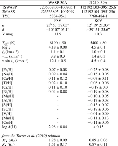
Table 1. Stellar parameters and abundances of our two primaries from spectral line analysis.
WASP-30A J1219–39A 1SWASP J235338.03–100705.1 J121921.03–395125.6 2MASS J23533805–1007049 J12192104–3951256 TYC 5834-95-1 7760-484-1 F8V K0V α 23h530 38.05” 12h190 21.03” δ −10◦ 070 05.1” −39◦ 510 25.6” V mag 11.9 10.3 Teff (K) 6190 ± 50 5400 ± 80 log g 4.18 ± 0.08 4.5 ± 0.1 ξt(km s−1) 1.1 ± 0.1 1.0 ± 0.1 vmac(km s−1) 3.8 ± 0.3 1.4 ± 0.3 vsin i?(km s−1) 12.1 ± 0.5 4.5 ± 0.4 [Fe/H] 0.07 ± 0.08 −0.23 ± 0.08 [Na/H] 0.09 ± 0.04 −0.15 ± 0.05 [Ca/H] 0.11 ± 0.12 −0.07 ± 0.11 [Ti/H] 0.02 ± 0.10 −0.08 ± 0.06 [Cr/H] 0.11 ± 0.10 −0.17 ± 0.0 [Ni/H] 0.04 ± 0.08 −0.19 ± 0.08 [Mg/H] - −0.10 ± 0.05 [Al/H] - −0.17 ± 0.08 [Si/H] - −0.13 ± 0.07 [Sc/H] - −0.18 ± 0.06 [V/H] - −0.01 ± 0.09 [Mn/H] - −0.11 ± 0.13 [Co/H] - −0.11 ± 0.06 log A(Li) 2.98 ± 0.04 < 0.15 from the Torres et al. (2010) relation
M?(M ) 1.28 ± 0.09 0.89 ± 0.06
R?(R ) 1.51 ± 0.17 0.87 ± 0.11
facilities used& number of observations used in the analysis WASP-South [V+R] 17 528 22 032
TRAPPIST [I+z] 571
-EulerCam [r’] 250
-CORALIE 32 61
HARPS 37
-Note: Spectral Type estimated from Teffusing the table in Gray (2008).
3. Data Treatment
3.1. the WASP-South photometry
We used standard aperture photometry as described in Section 4.3 of Pollacco et al. (2006) where a 3.5-pixel aperture around the source is used (with the source position taken from a catalogue). Sky subtraction comes from an annulus (with radii of 13 to 17 pixels). Regions around catalogued stars and cosmic rays are removed from that calculation. The pixel scale is 13.7” per pixel. To maximise photons, we observed in white light, only with a cut-off filter in the far red in order to reduce effects from fringing. This is a large bandpass approximating to V+R.
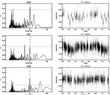
We used the sine-wave fitting method described in Maxted et al. (2011) to search for any periodicity in the WASP lightcurves owing to the rotation of the stars and caused by mag-netic activity, i.e., star spots. Spot-induced variability is not ex-pected to be coherent on long timescales as a consequence of the finite lifetime of star-spots and of differential rotation in the pho-tosphere so we analysed each season of WASP data separately.
Fig. 1. Left panels Periodograms for the WASP data from the different observing seasons for J1219–39. Horizontal lines in-dicate false alarm probability levels FAP=0.01 and vertical lines show our assumed rotational modulation period of P=10.6 d. The year of observation in given in the title. Right panels Lightcurves folded on the period P=10.61 d.
Table 2. Frequency analysis for J1219–39. N is the number of observations, P is the period corresponding to the strongest peak in the periodogram, Amp is the amplitude of the best-fit sine wave in milli-magnitudes and FAP is the false-alarm probability.
Year N P (day) Amp (mmag) FAP 2006 1855 10.710 6 0.027 2007 12104 5.292 5 0.004 2008 6019 10.300 3 0.001
We first subtracted a simple transit model from the lightcurve. We then calculated periodograms over 4096 uniformly spaced frequencies from 0 to 1.5 cycles/day (Fig. 1). The false-alarm probability levels shown in these figures are calculated using a boot-strap Monte Carlo method also described in Maxted et al. (2011).
For WASP-30 we analysed WASP lightcurves from 3 dif-ferent seasons with several thousand observations over about 100 days. These lightcurves show no significant periodic out-of-transit variability. We examined the distribution of amplitudes for the most significant frequency in each Monte Carlo trial and used these results to estimate a 95 % upper confidence limit of 0.8 milli-magnitude for the amplitude of any periodic signal in these lightcurves.
The results for our periodogram analysis of J1219–39 are shown in Table 2. Our interpretation is that we do detect rota-tional modulation of J1219−39 and that in the 2007 data the pat-tern of spots results in the strongest signal being seen at Prot/2,
where Protis the rotation period of the star at the latitude of the
star spots. This leads to Prot= 10.61±0.05 d calculated from the
unweighted mean and standard error on the mean from the three seasons. The periodograms for these data and the lightcurves folded on this value of Protare shown in Fig. 1.
3.2. the TRAPPIST I+ z-band photometry
A complete transit of WASP-30 was observed with the robotic 60cm telescope TRAPPIST1) (Gillon et al. 2011; Jehin et al. 2011). Located at La Silla ESO observatory (Chile), TRAPPIST is equipped with a 2K × 2K Fairchild 3041 CCD camera that has a 22’ × 22’ field of view (pixel scale= 0.64”/pixel). The transit of WASP-30 was observed on the night of 2010 October 15. The sky conditions were clear. We used the 1x2 MHz read-out mode with 1 × 1 binning, resulting in a typical read-out + overhead time and read noise of 8.2 s and 13.5 e−, respectively. The inte-gration time was 30s for the entire night. We observed through a special I+ z filter that has a transmittance of zero below 700nm, and > 90% from 750nm to beyond 1100nm. The telescope was defocused to average pixel-to-pixel sensitivity variations and to optimise the duty cycle, resulting in a typical full width at half-maximum of the stellar images of ∼6 pixels (∼3.8”). The posi-tions of the stars on the chip were maintained to within a few pixels over the course of two timeseries, separated by a merid-ian flip, thanks to the ‘software guiding’ system that regularly derives an astrometric solution from the most recently acquired image and sends pointing corrections to the mount if needed. After a standard pre-reduction (bias, dark, flat field), the stellar fluxes were extracted from the images using the IRAF/DAOPHOT aperture photometry software (Stetson 1987). Several sets of re-duction parameters were tested, and we kept the one giving the most precise photometry for the stars of brightness similar to WASP-30. After a careful selection of reference stars, di fferen-tial photometry was obtained (Gillon et al. 2012). The data are shown in figure 2. Because of a meridian flip inside the transit the photometry was analysed as two independent timeseries.
3.3. the radial velocity data
The spectroscopic data were reduced using the online Data Reduction Software (DRS) for the HARPS instrument. The radial-velocity information was obtained by removing the instru-mental blaze function and cross-correlating each spectrum with a mask. This correlation was compared with the Th–Ar spec-trum used as a wavelength-calibration reference (see Baranne et al. (1996) & Pepe et al. (2002) for details). The DRS has been shown to achieve remarkable precision (Mayor et al. 2009) thanks to a revision of the reference lines for thorium and argon by Lovis & Pepe (2007). A similar software package was used to prepare the CORALIE data. A resolving power R = 110 000 for HARPS provided a cross-correlation function (CCF) binned in 0.25 km s−1increments, while for the CORALIE data, with a
lower resolution of 50 000, we used 0.5 km s−1. The CCF
win-dow was adapted to be three times the size of the full width at half maximum (FWHM) of the CCF.
1 σ error bars on individual data points were estimated from photon noise alone. HARPS is stable in the long term to within 1 m s−1and CORALIE to better than 5 m s−1. These are smaller
than our individual error bars, and thus were not taken into ac-count.
As in the initial discovery paper, for WASP-30, a G2 mask was used. In the case of J1219–39 we used a K5 mask to extract the radial-velocity information.
Several points were removed from the analysis. For WASP-30, we excluded a mistakenly obtained series of 13 short CORALIE spectra taken during bad weather; the error bars are all above > 100 m s−1 when no other data has errors > 50
Triaud et al.: EBLM Project I - WASP-30b & J1219–39b −6000 −4000 −2000 0 2000 4000 6000 −0.4 −0.2 0.0 0.2 0.4 −50 0 50 Phase Radial Velocities (m s −1 ) O−C (m s −1 ) . . . . −50 0 50 −50 0 50 0.992 0.994 0.996 0.998 1.000 1.002 1.004 −0.04 −0.02 0.00 0.02 0.04 −0.004 −0.0020.000 0.002 0.004 RV (m s −1 ) O−C (m s −1 ) Flux O−C Phase . . . .
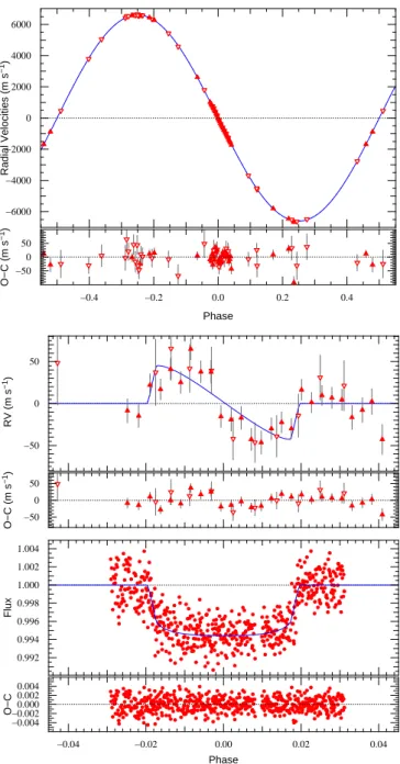
Fig. 2. top: Radial velocities on WASP-30 plotted with a circular Keplerian model and their residuals. CORALIE data is shown as inverted, empty, triangles. HARPS is show as upright trian-gles. Middle: zoom on the Rossiter–McLaughlin effect. Bottom: TRAPPIST I+ z photometry and model over-plotted. The inter-ruption of the observations is due to a telescope meridian flip.
m s−1. On SW1219–39b bad weather also affected observations,
notably during one of the Rossiter–McLaughlin sequences. All measurements with error bars > 20 m s−1 have been removed from the analysis as they show a clear jump in precision from other measurements. All the rejected radial velocities are nev-ertheless presented in the journal of observations, in the appen-dices, and are clearly indicated.
4. Spectral analysis
The analysis was performed following the methods detailed in Gillon et al. (2009b) with standard pipeline reduction products used in the analysis. The Hα line was used to determine the
−1.0 −0.5 0.0 0.5 1.0 10+4 −0.4 −0.2 0.0 0.2 0.4 −20 0 20 O−C (m s −1 ) Phase Radial Velocities (m s −1 ) . . . . −20 0 20 −20 0 20 0.96 0.98 1.00 1.02 −0.02 −0.01 0.00 0.01 0.02 −0.02 0.00 0.02 RV (m s −1 ) O−C (m s −1 ) Flux O−C Phase . . . .
Fig. 3. top: CORALIE radial velocities on J1219–39 plotted with an eccentric Keplerian model and their residuals. Middle: zoom on the Rossiter–McLaughlin effect. Bottom: WASP photometry and model over-plotted.
effective temperature (Teff). The surface gravity (log g) was
determined from the Ca i lines at 6162Å and 6439Å (Bruntt et al. 2010b), along with the Na i D lines. Additional Teff
and log g diagnostics were performed using the Fe lines. An ionisation balance between Fe i and Fe ii was required, along with a null dependence of the abundance on either equivalent width or excitation potential (Bruntt et al. 2008). The param-eters obtained from the analysis are listed in Table 1. The elemental abundances were determined from equivalent width measurements of several clean and unblended lines. A value for microturbulence (ξt) was determined from Fe i using the method
of Magain (1984). The quoted error estimates include that given by the uncertainties in Teff, log g and ξt, as well as the scatter
due to measurement and atomic data uncertainties.
A total of 37 individual HARPS spectra of WASP-30A were co-added to produce a single spectrum with a typical S/N of around 120:1. Interstellar Na D lines are present in the spectra with an equivalent widths of ∼0.16Å, indicating an extinction of E(B − V)= 0.05 using the calibration of Munari & Zwitter (1997). The projected stellar rotation velocity (v sin i?) was de-termined by fitting the profiles of several unblended Fe i lines. A value for macroturbulence (vmac) of 3.8 ± 0.3 km s−1was
as-sumed, based on the calibration by Bruntt et al. (2010a). An in-strumental FWHM of 0.07 ± 0.01 Å was determined from the telluric lines around 6300Å. A best fitting value of v sin i? =
12.1 ± 0.5 km s−1was obtained.
The lithium abundance would imply an age no more than ∼0.5 Gyr (Sestito & Randich 2005) but stars with Teffsimilar to
WASP-30A in M67 (5 Gyr old) have shown similar abundances (Fig. 6 in Sestito & Randich (2005)). Those results are in agreement with the analysis of 16 co-added CORALIE spectra that was published by Anderson et al. (2011b).
A similar analysis was conducted on J1219–39A. Individual spectra were combined to a single spectrum of S/N typically 150:1. Using a macroturbulence vmac= 1.4 ± 0.3 km s−1(Bruntt
et al. 2010a) we obtain a v sin i? = 4.5 ± 0.4 km s−1. Using the macroturbulence calibration from Valenti & Fischer (2005), we find vmac= 3.4 ± 0.3 km s−1, then we can infer v sin i? =
3.3 ± 0.4 km s−1. We will see later both those values are in contradiction with the V sin i?, directly measured from the
Rossiter–McLaughlin effect with the latter value being the closest. Here no Lithium can be detected for an equivalent width < 1mÅ. The cores of the Ca H & K lines show some emission indicative of stellar activity and in agreement with the detection of spot-induced variability (section 3.1).
We will make a distinction in this paper between v sin i?, the projected rotational velocity of the star computed by estimating the stellar line broadening, and the V sin i?, which is the same physical quantity, but obtained directly from the amplitude of the Rossiter–McLaughlin effect. We also distinguish i?the inclina-tion of the stellar spin, from i, the inclinainclina-tion of the orbital spin of the companion.
5. Model adjustment
Simple Keplerian models were fitted to the radial-velocity data simultaneously with transit models from Mandel & Agol (2002) fitted to the photometry, and a Rossiter–McLaughlin model by Gim´enez (2006) fitted to RV points falling within transit/eclipse. We used a quadratic limb-darkening law, and obtained param-eters from Claret (2004) to apply to the photometry. For the Rossiter–McLaughlin effect, we applied parameters derived by Claret for HARPS (Triaud et al. 2009). A Markov Chain Monte Carlo was used to compare the data and the models and explore parameter space to find the most likely model with robust confidence intervals on each parameter. Having only one set of parameters for all datasets ensures the parameter distributions are consistent with all of the data. The algorithm is widely described in several planet-discovery papers from the WASP consortium (e.g. Collier Cameron et al. (2007a); Gillon et al. (2009a); Anderson et al. (2011a); Triaud (2011a)). The same method is used here with one important difference:
While adjusting for planets, many authors have used the property that the mass of the planet is much less than the mass of the star (M2 << M?). This assumption is made in several
places: in calculating the mass ratio from the mass function, the radii from the scaled radii R2/a and R?/a, and in calculating the
stellar density ρ?. This last parameter is important since, being
more precise than the traditional log g, it is widely used to infer stellar parameters (Sozzetti et al. 2007).
Three methods are often used in the literature involving Markov Chain Monte Carlo fitting algorithms that use the mean stellar density to obtain M?. One can fit the transit to obtain ρ?, use it to infer the stellar mass by interpolating of stellar tracks, and then insert the new M?back into a chain, as employed by Hebb et al. (2009). Alternatively Enoch et al. (2010) have de-vised an empirical relation based on the Torres relation (Torres et al. 2010) which also delivers M?. Finally one can mix both previous methods and estimate M?at every step of an MCMC by
using ρ?to interpolate within theoretical stellar tracks as shown in Triaud (2011a) and in Gillon et al. (2012). ρ?is defined, from
Kepler’s law as: M? R3? = 4π2 GP2 a R? !3 − M2 R3? (1)
In our case, the second term can no longer be considered null. In order to still be able to use the more precise ρ?over log g,
we proceeded as follow: for every step in the MCMC we use the transit geometry to estimate the secondary’s orbital inclination i. Then the mass function (Hilditch 2001)
f(m)= (1 − e2)3/2P K
3
2π G (2)
is estimated. It can also be written as f(m)= (M2 sin i)
3
(M?+ M2)2
. (3)
Equating both, we can numerically solve for M2 assuming
M? (for example at the start of the chain, from the Torres
relation). The orbital separation can then be estimated, and, having R?/a from the transit signal, we obtain R?. We thus have gathered first estimates of all quantities necessary to compute ρ?. This value is then combined with [Fe/H] and Teff to give
M? from interpolating within stellar evolution tracks. M? can
then be used to re-estimate M2 and R?, via the same path as
outlined above, from which R2 is also determined, using the
transit depth. This is repeated for each of the 2 000 000 steps of our MCMCs.
We use a new version of the Geneva stellar evolution tracks, described in Mowlavi et al. (2012) and for the moment make the assumption that the primary is located on the main sequence. Because the steps falling outside the tracks are rejected, and pro-vided the star is indeed on the main sequence, fitting using the tracks has the advantage of only allowing physically possible stars to be used in the MCMC. It has also the capacity to check and refine stellar parameters derived from spectral analysis, es-pecially with respect to the lower boundary composed by the zero age main sequence.
Our Markov chains use the following jump parameters: D, the photometric transit/eclipse depth, W, its width, b, the impact parameter, K, the semi-amplitude of the radial velocity signal, P, the period, T0, the transit mid-time point at the barycentre of
Triaud et al.: EBLM Project I - WASP-30b & J1219–39b
the data (RV and photometric, weighted by their respective sig-nal to noise). We also have two pairs of parameters: √ecos ω & √ecos ω and √Vsin I sin β & √Vsin I cos β where e is the eccentricity, ω is the angle of periastron, V sin I is the rota-tion velocity of the star and β is the projected spin-orbit an-gle. Those parameters are combined together to avoid inserting a bias in the determination of e and V sin I (see Ford (2006); Triaud et al. (2011) for details). [Fe/H] and Teff are drawn
ran-domly from a normal distribution taken from our spectral anal-ysis. Normalisation factors for the photometry, and γ velocities for each RV datasets, are not floating, but computed. For WASP-30, the RV data was cut into four datasets: the CORALIE data on the orbit, the CORALIE data during RM effect plus one mea-surement the night before and after, the HARPS data on the or-bit, the HARPS RM effect plus one point the night before, and one the night after. Several chains are run to ensure, first, that convergence is achieved, but also to test the effects of different priors.
From the jump parameters a number of physical parameters, such as the masses and radii of both objects, can be computed. Useful, assumption-free parameters are also available, such as the secondary’s surface gravity log g2, as noted in Southworth
et al. (2004).
Results are taken as the modes of the posterior probability distributions. Errors for each parameter are obtained around the mode using the marginalised distribution and taking the 1-, 2-and 3-σ confidence regions.
6. Results
6.1. WASP-30b
Several chains were run on WASP-30b, exploring the effect that various priors could have on the end results. Overall the fit between the data and the models is good. In order to get a χ2
reduced close to 1, an extra contribution of 5 m s
−1 was added
quadratically to the errors of the radial-velocity data. This stems mostly from one point in the HARPS data as well as from some high-cadence noise during the Rossiter–McLaughlin sequence. Nevertheless, we achieve a dispersion after the models are sub-tracted of 26.8 m s−1for a χ2
reduced= 1.47 ± 0.21.
The main difference between this analysis and that presented by Anderson et al. (2011b) is a slight change in mass and ra-dius of WASP-30b, arising from different choices for the es-timation of the primary’s parameters. Anderson et al. (2011b) used a Main-Sequence prior, which forced the photometric fit to be compatible with a smaller and less massive star. Upon re-laxing the prior, those authors obtain a solution for the primary that is close to ours. The Main-Sequence prior is also the reason for a slightly different transit duration between the discovery pa-per and the current solution. It forced a solution through the ini-tial data which is no longer compatible with the addition of the TRAPPIST light curve. The data in the discovery paper only had WASP photometry and an Euler light curve that was imprecise during ingress. A small additional contribution comes from no longer making the planet approximation.
Using priors on the values of M?and R?obtained using the
Torres relation does not affect the result. Fits not using them are thus preferable as they constitute an independent measurement. WASP-30A is found to be a 1.25 ± 0.03 M , 1.39 ± 0.03 R star
at the end of its main-sequence lifetime. The values for Teff and
[Fe/H] from the output of the MCMC (table 3) are entirely com-patible with those presented in Table 1, meaning that we suf-fer little bias due to proximity of the star to the terminal-age
Table 3. Floating and computed parameters found for our two systems WASP-30A&b and J1219–39A&b. For clarity only the last two digits of the 1 σ errors are shown.
Parameters (units) WASP-30 J1219–39 jump parameters P(days) 4.156739+(12)−(10) 6.7600098+(34)−(22) T0(BJD-2 450 000) 5443.06046+(43)−(33) 5187.72676 +(29) −(41) D 0.00494+(11)−(13) 0.02088+(89)−(69) W(days) 0.1644+(13)−(09) 0.1040+(20)−(20) b(R?) 0.10+(0.12)−(0.10) 0.733+(2)−(31) K(m s−1) 6606.7+(4.7) −(5.3) 10 822.2 +(2.8) −(3.1) √ V sin I cos β 3.40+(0.12)−(0.24) 1.61+(0.13)−(0.11) √ V sin I sin β 0.5+(1.1)−(1.6) 0.13+(0.13)−(0.15) √ ecos ω 0 (fixed) 0.21932+(57)−(48) √ esin ω 0 (fixed) 0.08537+(85)−(89) derived parameters f(m) (M ) 0.00012418+(28)−(29) 0.000883709+(71)−(71) R2/R? 0.0704+(07)−(10) 0.1446 +(29) −(25) R?/a 0.1164+(25)−(12) 0.0561+(18)−(23) ρ?(ρ ) 0.466+(16)−(29) 1.50+(0.17)−(0.17) R?(R ) 1.389(33)(25) 0.811+(38)−(24) M?(M ) 1.249+(32)−(36) 0.826+(32)−(29) log g?(cgs) 4.250+(09)−(18) 4.523+(39)−(26) R2/a 0.00821+(19)−(18) 0.00817 +(33) −(48) R2(RJup) 0.951+(28)−(24) 1.142+(69)−(49) M2(MJup) 62.5+(1.2)−(1.2) 95.4 +(1.9) −(2.5) log g2(cgs) 5.234+(19)−(22) 5.245 +(47) −(42) a(AU) 0.05534+(47)−(51) 0.06798+(83)−(77) i(◦ ) 89.43+(0.51)−(0.93) 87.61+(0.17)−(0.18) β (◦ ) 7+(19)−(27) 4.1+(4.8)−(5.3) e < 0.0044 0.05539+(23)−(22) ω (◦ ) - 21.26+(0.21)−(0.23) | ˙γ| (m s−1yr−1) < 53 < 10 V sin i?(km s−1) 12.1+(0.4) −(0.5) 2.61 +(42) −(35) Teff(K) 6202+(42)−(51) 5412 +(81) −(65) [Fe/H] 0.083+(69)−(50) -0.209+(70)−(75) Age (Gyr) 3.4+(0.3)−(0.5) 6-12 γcoralie(km s−1) 7.9307+(22)−(17) 33.7971 +(16) −(15) γharps(km s−1) 7.87472+(36)−(31)
-main sequence. Thus, using these stellar parameters we find that WASP-30b is a 62.5 ± 1.2 MJupbrown dwarf with a radius of
0.95 ± 0.03 RJup. No eccentricity is detected. We can place a
95 %-confidence upper limit of e < 0.0044. No additional ac-celeration is detected either. We calculated an upper constraint of | ˙γ| < 53 m s−1yr−1.
The second feature of interest is the Rossiter–McLaughlin effect. Because of a low impact parameter the known degeneracy between V sin I, β and b does not yield an unique solution (see
a) b) d) c) 0.00 0.02 60 62 64 66 68 1.20 1.25 1.30 1.35 1.40 0.00 0.02 Ms (M sol ) M2 (Mjup) . . . . 0.00 0.02 1.15 1.2 1.25 1.3 1.35 1.15 1.2 1.25 1.3 1.35 6000 6100 6200 6300 6400 1.3 1.4 1.5 0.00 0.05 ρ − 1/3 ( ρsol ) Teff (K) . . . . 0.00 0.02 60 62 64 66 68 0.9 1.0 1.1 1.2 1.3 0.00 0.05 R2 (R jup ) M2 (Mjup) . . . . 0.00 0.01 −60 −40 −20 0 20 40 60 10 11 12 13 14 0.00 0.02 β (o) V sin I (km s − 1) . . . .
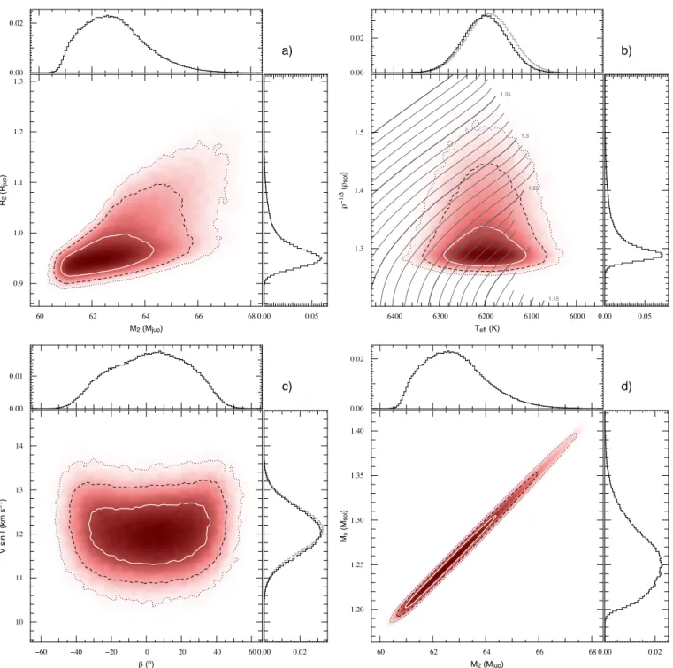
Fig. 4. WASP-30: The central panels show posterior probability-density distributions from the MCMC output, with contours at the 1-, 2- and 3-σ confidence regions. The side panels show marginalised distributions as histograms in black. Where used, the priors are shown in grey. Panel (a) radius and mass of WASP-30b. b) modified Hertzsprung–Russell diagram over-plotted with the Geneva evolution tracks. Masses are indicated in M . c) V sin i? versus β from fitting the Rossiter–McLaughlin effect. d) dependence of
the secondary’s mass on our incomplete knowledge of the primary mass.
for example Albrecht et al. (2011b) or Triaud et al. (2011)). The application of a prior on V sin I, using the value measured from spectral line broadening, prevents the MCMC from searching unphysical values of V sin I. It also restricts the impact param-eter b from wandering too much, which otherwise was slightly affecting ρ? and thus the primary’s mass and radius. We thus select the solutions using that prior. Full results are available in Table 3.
WASP-30b is in a prograde orbit. Using the posterior distri-bution obtained for the stellar radius and the V sin i?, the
rota-tion period of the star is estimated at 5.9 ± 0.3 days, away from synchronisation. Any attempt to use higher values for V sin i?
would result in forcing the fit towards an inclined orbit.
6.2. J1219–39b
The overall fit for J1219–39 is good: we obtain χ2= 82.4 ± 12.8
for 61 radial velocity points giving χ2reduced = 1.53 ± 0.23 with-out adding a jitter to the radial velocities. Errors on the pho-tometry were adjusted to obtain a χ2reduced = 1. The
imposi-Triaud et al.: EBLM Project I - WASP-30b & J1219–39b a) b) d) c) 0.00 0.02 0.04 −20 −10 0 10 20 30 1 2 3 4 0.00 0.02 β (o) V sin I (km s − 1) . . . . 0.00 0.02 5.45 5.50 5.55 5.60 5.65 10−2 20.5 21.0 21.5 22.0 0.00 0.02 ω ( o) e . . . . 0.00 0.02 0.04 0.7 0.75 0.8 0.8 0.85 0.85 0.9 0.95 5200 5400 5600 5800 0.75 0.80 0.85 0.90 0.95 1.00 0.00 0.02 ρ − 1/3 ( ρsol ) Teff (K) . . . . 0.00 0.02 90 95 100 105 1.0 1.1 1.2 1.3 1.4 1.5 0.00 0.02 R2 (R jup ) M2 (Mjup) . . . .
Fig. 5. J1219–39: The central panels show posterior probability-density distributions from the MCMC output, with contours at the 1-, 2- and 3-σ confidence regions. The side panels show marginalised distributions as histograms in black. Where used, the priors are shown in grey. Panel (a) radius and mass of J1219–39b. b) modified Hertzsprung–Russell diagram over-plotted with the Geneva evolution tracks. Masses are indicated in M . c) V sin i?versus β from fitting the Rossiter–McLaughlin effect. d) the eccentricity e
and argument of periastron ω.
tion of priors using the Torres relation on M?and R?does not
affect the results. We thus adopt a prior-free chain. From the eclipse and spectroscopy, without any assumptions, we obtained log g2= 5.25±0.05 indicating that an unresolved dense object is
orbiting the primary. After careful analysis we find that J1219– 39A is a 0.83 ± 0.03 M , 0.81 ± 0.03 R star and its companion
is a low mass star, of 0.091 ± 0.002 M and 0.117 ± 0.006 R
(95 ± 2 MJupand 1.14 ± 0.05 RJup). The orbit is slightly eccentric
(e = 0.0554 ± 0.0002) while β = 4◦± 5, showing good spin– orbit alignment. Full results are presented in Table 3. Here too
we do not detect any additional acceleration and can place an upper constraint with | ˙γ| < 10 m s−1yr−1.
Claims of low eccentricities have been disputed in the past (Lucy & Sweeney 1971). Now, thanks to the high precision achieved with radial velocities, it is possible to measure ex-tremely small orbital eccentricities. As a rule of thumb, one cannot conclusively detect eccentricity if the difference between the circular and eccentric model is smaller than the RMS of the residuals. This difference can be approximated by 2 e K. In our case we are well above that value. We nevertheless forced a
0.00 0.02 1.5 2.0 2.5 3.0 3.5 4.0 1.20 1.25 1.30 1.35 1.40 0.00 0.02 Age (Gyr) Ms (M sol ) . . . .
Fig. 6. The central panel shows the posterior probability-density distribution for stellar age against stellar mass for WASP-30. The contours show the 1-, 2- and 3-σ confidence regions; the side panels show the marginalised distributions as histograms. The data derive from interpolating using the mean stellar den-sity, Teffand metallicity, into the Geneva stellar evolution tracks
(Mowlavi et al. 2012).
circular model and find a much poorer fit reflected in a χ2 =
46 217 ± 304 instead of χ2= 62.2 ± 11.1 for the eccentric model (on the 42 points not affected by the RM effect).
From fitting the Rossiter–McLaughlin effect we obtain an independent (prior-free) distribution for stellar rotation peaking at V sin I = 2.6 ± 0.4 km s−1. This value is significantly
dif-ferent from the value of v sin i? presented in Table 1 and ob-tained from stellar line broadening. If we use v sin i?as a prior on V sin i?, the fit of the Rossiter–McLaughlin effect worsens
slightly, but stays within the natural noise variability. Under this prior, the most likely value becomes V sin I = 3.6 ± 0.3, in be-tween the independent values. This matches the value of v sin i?
obtained when using a macroturbulence value from Valenti & Fischer (2005) instead of from Bruntt et al. (2010a). We adopt the value of V sin I found from the Rossiter–McLaughlin effect alone, as it is a directly measured value, one that can be tested against macroturbulence laws.
Assuming coplanarity (i= i?) as indicated by β and using the MCMC’s posterior probabilities and the RM’s V sin i?, J1219– 39A would have a rotation period of 15.2±2.1 days. The solution using a prior on V sin i?gives a period of rotation of 11.7 ± 1.0
days, while when using instead the value of v sin i? in Table 1 we obtain 9.0 ± 0.9 days. Since none of these is compatible with the orbital period, we have neither synchronisation between the secondary’s orbital motion and the primary’s rotation, nor pseudo-synchronisation.
An analysis of the out-of-transit WASP data shows a recur-ring frequency at about 10.6 days on three seasons of data, pre-sumably due to the rotation of stellar spots on the surface of the primary (see section 3.1). This fourth possible rotation period is a direct observable. The discrepancy with the value obtained
us-ing the V sin i? is not understood, yet is interesting to note2.
Further comparison between the V sin i? from the Rossiter–
McLaughlin and photometric rotation periods seems warranted.
7. Discussion & Conclusions
We announce the discovery of a new low-mass star whose mass and radius have been precisely measured and found to be at the junction between the stellar and substellar regimes. In addi-tion, using observations with the CORALIE spectrograph, on the 1.2 m Euler Telescope, and HARPS, on the ESO 3.6 m, we have demonstrated the detection of the Rossiter–McLaughlin effect on two objects more massive than planets. These measurements are amongst the first to be realised on such objects. They will help study the dynamical events that could have led to the for-mation of binary systems where both components have a large mass difference, and may also provide a useful comparison sam-ple to the spin–orbit angle distribution of hot Jupiters, as well as helping theoretical developments in the treatment of tides, the main mechanism behind synchronisation, circularisation and re-alignment.
H´ebrard et al. (2011) and Moutou et al. (2011) note that while hot Jupiters are usually found with a large variety of orbital angles, objects above 5 Mjupare not found on retrograde
orbits. We extend the distribution of spin–orbit angle versus mass to beyond the planetary range. Both of our objects appear well aligned with their primary, further confirming that trend. Being around stars colder than 6250 K, they also reinforce the pattern shown by Winn et al. (2010) between orbital inclination and the primary’s effective temperature. The age of WASP-30A and the alignment of WASP-30b also helps strengthen the pattern claimed in Triaud (2011b) that systems older than 2.5–3 Gyr are predominantly aligned. It is interesting to note that while J1219–39b is on a slightly eccentric orbit, its orbital spin is aligned with its primary’s rotational spin. This gives observational evidence that orbital realignment may be faster than orbital circularisation for these objects, in opposition with planets. Final tidal equilibrium has not been reached for either system as WASP-30A is not synchronised and J1219–39b is not circularised (nor synchronised) (Hut 1980).
While not being the primary objective of this paper, we present a method to analyse, in a global manner, eclipse pho-tometry, the radial-velocity reflex motion, and the Rossiter– McLaughlin effect, for objects more massive than planets, in or-der to obtain precise estimates of the mass, radius and orbital parameters of SB1s. The precision of a few percent that we ob-tain comes from our use of ρ?, the mean stellar density, instead of the more traditional log g when interpolating inside the stel-lar evolution tracks. This interpolation gives us precise values for the primary’s stellar parameters which are used to estimate the secondary’s parameters. We can check our method by deduc-ing log g?and comparing them to their spectral counterpart. The values are in very good agreement and fall within the errors of the spectral method (see table 6). This method also allows us to estimate ages from reading the stellar tracks, something impor-tant in the case of close binaries where gyrochronology cannot be trusted owing to the tidal evolution of the system.
Our low-mass eclipsing objects have very similar surface gravities, but, located on opposite sides of the brown-dwarf limit,
2 this could lead to presume i
?= 42◦± 8, indicating spin–orbit mis-alignment. The discrepancy between the different values of equatorial velocities prevents us from being sure.
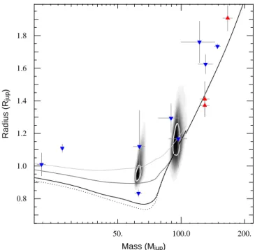
Triaud et al.: EBLM Project I - WASP-30b & J1219–39b 100.0 200. 50. 0.8 1.0 1.2 1.4 1.6 1.8 Radius (R jup ) Mass (Mjup) . . . .
Fig. 7. Mass–radius diagram for heavy planets, brown dwarfs and low-mass stars. The radius axis corresponds to the size range of Jupiter-mass planets discovered so far. Inverted blue triangles show eclipsing/transiting SB1s, upright red triangles denote in-terferometric measurements. The two (M2, R2) posterior
prob-ability density distributions for WASP-30b and J1219–39b are drawn in grey with their 1 − σ confidence regions in white. Models by Baraffe et al. (2003, 1998) are also displayed with ages 5 Gyr (black), 1 Gyr (dark grey), 500 Myr (light grey) and 10 Gyr (dotted). Models are for [M/H] = 0. Observational data were taken from Lane et al. (2001); S´egransan et al. (2003); Pont et al. (2005a,b, 2006); Beatty et al. (2007); Deleuil et al. (2008); Demory et al. (2009); Bouchy et al. (2011); Johnson et al. (2011); Ofir et al. (2012); Siverd et al. (2012).
have sizes dominated by different physics (Baraffe et al. 2003). Plotting the posterior probability distribution for the mass and radius on theoretical mass–radius relations (Baraffe et al. 2003, 1998) in Figure 7, we observe that WASP-30b is between the 0.5 and 1 Gyr tracks, suggesting the object is fairly young (and thus luminous, which should cause a measurable secondary eclipse). This is at odds with the age of the primary, which we have found to be older than 2 Gyr with 99% confidence, with a best age of 3.4 ± 0.4 Gyr (figure 6).
We could explain this radius anomaly if the object has been inflated in the same manner that has been observed for hot Jupiters thanks to the high irradiation received from its primary (Demory & Seager 2011). The exact physical causes are still be-ing debated. It may also be that energy has been stored inside the object if it circularised from a previously highly eccentric orbit (Mazeh & Shaham 1979; Fabrycky & Tremaine 2007). WASP-30b’s mass is interesting in that it is close to the minimum of the tracks presented in Baraffe et al. (2003) and displayed in fig-ure 7. The mass–radius posterior distribution of J1219–39b is compatible with the 10-Gyr theoretical line. Better photometry would help to reduce the confidence region. This analysis will be the subject of subsequent papers (Hebb et al. in prep). One could object that our analysis does not take into account the fact that both WASP-30b and J1219–39b are self luminous. Even in
the case that they had the same effective temperature as their primaries, the overall contamination cannot be larger than their relative sizes ∼ 1 %, lower than our current precision.
We would like to attract the attention on the fact that both those objects have sizes entirely compatible with those of hot Jupiters. While hot Jupiters are often inflated, Jupiter-mass planets at longer periods no longer are (Demory & Seager 2011). It would then be expected that many of the planet candidates published by the space mission Kepler with inflated radii (> 1.2 RJup) and periods longer than 10–15 days could be
objects similar to WASP-30b and J1219–39b. While not being planets, they are of great interest for their masses, radii and orbital parameters.
Finally, the Rossiter–McLaughlin effect has recently been used almost exclusively to measure planetary orbital planes. Observing it for binary stars extends that work by bridging the gap in mass ratio between planetary and stellar systems. Comparison between low-mass binaries in our case with higher-mass binaries as in the BANANA survey (Albrecht et al. 2011a) will permit us to test different regimes of binary formation and tidal interactions.
Yet more information still lies in the study of this RV anomaly. Its use in the beginning of the 20th century was pri-marily to measure the rotation of stars. As seen in this paper, there is a discrepancy between the v sin i?values obtained by
using calibration of the macroturbulence and the directly mea-sured V sin i? from the Rossiter–McLaughlin effect. This was
also pointed out in Triaud et al. (2011) in the case of WASP-23, and by Brown et al. (2012) in the case of WASP-16. Both those systems, like J1291–39, contain K dwarfs, and both had their spectroscopic v sin i?overestimated compared to the value ob-tained via the Rossiter–McLaughlin effect. Since we compute the spin–orbit angle β and the V sin i?, we have strong con-straints on the coplanarity of the system and rotation velocity of the primary; thanks to the transit/eclipse geometry, we ob-tain accurate and precise masses and radii for both the primary and the secondary. Combining all this information and collecting many measurements, we will be able to test which of the macro-turbulence laws one should use. Should none apply, inserting the observed V sin i?values as input parameters in spectral line analyses we will have the capacity to measure macroturbulence directly. Observing the Rossiter–McLaughlin effect is thus not just about glimpsing into the past dynamical history of systems, but can also become an important tool for understanding stellar physics better.
Nota Bene We used the UTC time standard and Barycentric Julian Dates in our analysis. Our results are based on the equa-torial solar and jovian radii and masses taken from Allen’s Astrophysical Quantities.
Acknowledgements. The authors would like to acknowledge the use of ADS and of Simbad at CDS. We also would like to attract attention on the help and kind attention of the ESO staff at La Silla and at the guesthouse in Santiago as well as on the dedication of the many observers whose efforts during many nights were required to obtain all the data presented here. Special thanks go to our pro-grammers and their wonderful automatic Data Reduction Software, allowing us to observe live (!) an object transiting its primary (be it planet, brown dwarf or M dwarf), thus makes observing so much more exciting. We thank Kris Hełminiak for commenting on the draft and generally for being a nice guy. Thanks also go to Brice-Oliver Demory for his help with regards with interferometric masses and radii measurements of low-mass stars and the inspiration he provided to AT for starting to seek brown dwarfs, which led to the discovery of those many low-mass binaries. This work is supported financially by the Swiss Fond National de Recherche Scientifique.
References
Albrecht, S., Reffert, S., Snellen, I., Quirrenbach, A., & Mitchell, D. S. 2007, A&A, 474, 565
Albrecht, S., Reffert, S., Snellen, I. A. G., & Winn, J. N. 2009, Nature, 461, 373 Albrecht, S., Winn, J. N., Carter, J. A., Snellen, I. A. G., & de Mooij, E. J. W.
2011a, ApJ, 726, 68
Albrecht, S., Winn, J. N., Johnson, J. A., et al. 2011b, ApJ, 738, 50
Anderson, D. R., Collier Cameron, A., Hellier, C., et al. 2011a, A&A, 531, A60 Anderson, D. R., Collier Cameron, A., Hellier, C., et al. 2011b, ApJ, 726, L19 Baraffe, I., Chabrier, G., Allard, F., & Hauschildt, P. H. 1998, A&A, 337, 403 Baraffe, I., Chabrier, G., Barman, T. S., Allard, F., & Hauschildt, P. H. 2003,
A&A, 402, 701
Baranne, A., Queloz, D., Mayor, M., et al. 1996, A&AS, 119, 373 Beatty, T. G., Fern´andez, J. M., Latham, D. W., et al. 2007, ApJ, 663, 573 Bentley, S. J., Smalley, B., Maxted, P. F. L., et al. 2009, A&A, 508, 391 Bouchy, F., Deleuil, M., Guillot, T., et al. 2011, A&A, 525, A68
Brown, D. J. A., Cameron, A. C., Anderson, D. R., et al. 2012, MNRAS, 423, 1503
Bruntt, H., Bedding, T. R., Quirion, P.-O., et al. 2010a, MNRAS, 405, 1907 Bruntt, H., De Cat, P., & Aerts, C. 2008, A&A, 478, 487
Bruntt, H., Deleuil, M., Fridlund, M., et al. 2010b, A&A, 519, A51 Caballero, J. A., B´ejar, V. J. S., Rebolo, R., et al. 2007, A&A, 470, 903 Claret, A. 2004, A&A, 428, 1001
Collier Cameron, A., Bouchy, F., H´ebrard, G., et al. 2007a, MNRAS, 375, 951 Collier Cameron, A., Wilson, D. M., West, R. G., et al. 2007b, MNRAS, 380,
1230
Deleuil, M., Deeg, H. J., Alonso, R., et al. 2008, A&A, 491, 889 Demory, B.-O. & Seager, S. 2011, ApJS, 197, 12
Demory, B.-O., S´egransan, D., Forveille, T., et al. 2009, A&A, 505, 205 Desmet, M., Fr´emat, Y., Baudin, F., et al. 2010, MNRAS, 401, 418 Doyle, L. R., Carter, J. A., Fabrycky, D. C., et al. 2011, Science, 333, 1602 Enoch, B., Collier Cameron, A., Parley, N. R., & Hebb, L. 2010, A&A, 516, A33 Fabrycky, D. & Tremaine, S. 2007, ApJ, 669, 1298
Fernandez, J. M., Latham, D. W., Torres, G., et al. 2009, ApJ, 701, 764 Ford, E. B. 2006, ApJ, 642, 505
Gaudi, B. S. & Winn, J. N. 2007, ApJ, 655, 550
Gillon, M., Anderson, D. R., Triaud, A. H. M. J., et al. 2009a, A&A, 501, 785 Gillon, M., Jehin, E., Magain, P., et al. 2011, Detection and Dynamics
of Transiting Exoplanets, St. Michel l’Observatoire, France, Edited by F. Bouchy; R. D´ıaz; C. Moutou; EPJ Web of Conferences, Volume 11, id.06002, 11, 6002
Gillon, M., Smalley, B., Hebb, L., et al. 2009b, A&A, 496, 259 Gillon, M., Triaud, A. H. M. J., Fortney, J. J., et al. 2012, ArXiv e-prints Gim´enez, A. 2006, ApJ, 650, 408
Gray, D. F. 2008, The Observation and Analysis of Stellar Photospheres, ed. Gray, D. F.
Hebb, L., Collier-Cameron, A., Loeillet, B., et al. 2009, ApJ, 693, 1920 H´ebrard, G., Bouchy, F., Pont, F., et al. 2008, A&A, 488, 763 H´ebrard, G., Ehrenreich, D., Bouchy, F., et al. 2011, A&A, 527, L11
Hilditch, R. W. 2001, An Introduction to Close Binary Stars, ed. Hilditch, R. W. Holt, J. R. 1893, Astro-Physics, XII, 646
Hosokawa, Y. 1953, PASJ, 5, 88
Hube, D. P. & Couch, J. S. 1982, Ap&SS, 81, 357 Hut, P. 1980, A&A, 92, 167
Hut, P. 1981, A&A, 99, 126
Jehin, E., Gillon, M., Queloz, D., et al. 2011, The Messenger, 145, 2 Johnson, J. A., Apps, K., Gazak, J. Z., et al. 2011, ApJ, 730, 79 Kopal, Z. 1942a, ApJ, 96, 399
Kopal, Z. 1942b, Proceedings of the National Academy of Science, 28, 133 Kozai, Y. 1962, AJ, 67, 579
Lane, B. F., Boden, A. F., & Kulkarni, S. R. 2001, ApJ, 551, L81 L´opez-Morales, M. 2007, ApJ, 660, 732
Lovis, C. & Pepe, F. 2007, A&A, 468, 1115 Lucy, L. B. & Sweeney, M. A. 1971, AJ, 76, 544 Magain, P. 1984, A&A, 134, 189
Malmberg, D., Davies, M. B., & Heggie, D. C. 2011, MNRAS, 411, 859 Malmberg, D., de Angeli, F., Davies, M. B., et al. 2007, MNRAS, 378, 1207 Mandel, K. & Agol, E. 2002, ApJ, 580, L171
Matsumura, S., Peale, S. J., & Rasio, F. A. 2010a, ApJ, 725, 1995
Matsumura, S., Thommes, E. W., Chatterjee, S., & Rasio, F. A. 2010b, ApJ, 714, 194
Maxted, P. F. L., Anderson, D. R., Collier Cameron, A., et al. 2011, PASP, 123, 547
Mayor, M., Udry, S., Lovis, C., et al. 2009, A&A, 493, 639 Mazeh, T. & Shaham, J. 1979, A&A, 77, 145
McLaughlin, D. B. 1924, ApJ, 60, 22
Morales, J. C., Gallardo, J., Ribas, I., et al. 2010, ApJ, 718, 502
Morales, J. C., Ribas, I., & Jordi, C. 2008, A&A, 478, 507 Morales, J. C., Ribas, I., Jordi, C., et al. 2009, ApJ, 691, 1400 Mordasini, C., Alibert, Y., & Benz, W. 2009, A&A, 501, 1139 Moutou, C., D´ıaz, R. F., Udry, S., et al. 2011, A&A, 533, A113 Mowlavi, N., Eggenberger, P., Meynet, G., et al. 2012, A&A, 541, A41 Munari, U. & Zwitter, T. 1997, A&A, 318, 269
Nagasawa, M., Ida, S., & Bessho, T. 2008, ApJ, 678, 498
Naoz, S., Farr, W. M., Lithwick, Y., Rasio, F. A., & Teyssandier, J. 2011, Nature, 473, 187
Ofir, A., Gandolfi, D., Buchhave, L., et al. 2012, MNRAS, 423, L1 Pepe, F., Mayor, M., Rupprecht, G., et al. 2002, The Messenger, 110, 9 Pollacco, D. L., Skillen, I., Collier Cameron, A., et al. 2006, PASP, 118, 1407 Pont, F., Bouchy, F., Melo, C., et al. 2005a, A&A, 438, 1123
Pont, F., Melo, C. H. F., Bouchy, F., et al. 2005b, A&A, 433, L21 Pont, F., Moutou, C., Bouchy, F., et al. 2006, A&A, 447, 1035 Queloz, D., Eggenberger, A., Mayor, M., et al. 2000, A&A, 359, L13 Rasio, F. A. & Ford, E. B. 1996, Science, 274, 954
Rossiter, R. A. 1924, ApJ, 60, 15
Schlesinger, F. 1910, Publications of the Allegheny Observatory of the University of Pittsburgh, 1, 123
S´egransan, D., Kervella, P., Forveille, T., & Queloz, D. 2003, A&A, 397, L5 Sestito, P. & Randich, S. 2005, A&A, 442, 615
Siverd, R. J., Beatty, T. G., Pepper, J., et al. 2012, ArXiv e-prints
Slettebak, A. 1985, in IAU Symposium, Vol. 111, Calibration of Fundamental Stellar Quantities, ed. D. S. Hayes, L. E. Pasinetti, & A. G. D. Philip, 163– 183
Southworth, J., Zucker, S., Maxted, P. F. L., & Smalley, B. 2004, MNRAS, 355, 986
Sozzetti, A., Torres, G., Charbonneau, D., et al. 2007, ApJ, 664, 1190 Stetson, P. B. 1987, PASP, 99, 191
Struve, O. 1950, Stellar evolution, an exploration from the observatory., ed. Struve, O.
Thies, I., Kroupa, P., Goodwin, S. P., Stamatellos, D., & Whitworth, A. P. 2011, MNRAS, 417, 1817
Tokovinin, A., Thomas, S., Sterzik, M., & Udry, S. 2006, A&A, 450, 681 Torres, G., Andersen, J., & Gim´enez, A. 2010, A&A Rev., 18, 67
Triaud, A. H. M. J. 2011a, PhD thesis, Observatoire Astronomique de l’Universite de Geneve, http://archive-ouverte.unige.ch/unige:18065 Triaud, A. H. M. J. 2011b, A&A, 534, L6
Triaud, A. H. M. J., Collier Cameron, A., Queloz, D., et al. 2010, A&A, 524, A25
Triaud, A. H. M. J., Queloz, D., Bouchy, F., et al. 2009, A&A, 506, 377 Triaud, A. H. M. J., Queloz, D., Hellier, C., et al. 2011, A&A, 531, A24 Udalski, A. 2007, in Astronomical Society of the Pacific Conference Series, Vol.
366, Transiting Extrapolar Planets Workshop, ed. C. Afonso, D. Weldrake, & T. Henning, 51
Valenti, J. A. & Fischer, D. A. 2005, ApJS, 159, 141
Winn, J. N., Albrecht, S., Johnson, J. A., et al. 2011, ApJ, 741, L1
Winn, J. N., Fabrycky, D., Albrecht, S., & Johnson, J. A. 2010, ApJ, 718, L145 Winn, J. N., Johnson, J. A., Albrecht, S., et al. 2009, ApJ, 703, L99
Winn, J. N., Noyes, R. W., Holman, M. J., et al. 2005, ApJ, 631, 1215 Worek, T. F. 1996, PASP, 108, 962
Wu, Y. & Lithwick, Y. 2011, ApJ, 735, 109
Wu, Y., Murray, N. W., & Ramsahai, J. M. 2007, ApJ, 670, 820 Young, P. & Schneider, D. P. 1980, ApJ, 238, 955
Triaud et al.: EBLM Project I - WASP-30b & J1219–39b
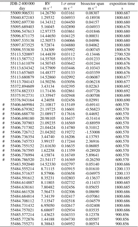
Table .1. CORALIE radial velocities on WASP-30. Points excluded from the analysis are marked by #.
JDB-2 400 000 RV 1 σ error bissector span exposition time day m s−1 m s−1 m s−1 s 55009.906531 14.26750 0.03161 0.08307 1800.687 55040.872183 1.29532 0.04933 -0.18938 1800.683 55092.697730 14.34312 0.04450 0.04157 1800.680 55095.689403 5.16045 0.02890 -0.04933 1800.678 55096.547613 12.97375 0.03861 -0.01846 1800.680 55096.871175 14.44650 0.04125 0.00031 1800.680 55097.535138 12.50573 0.04066 0.04896 1800.680 55097.873525 9.72874 0.04880 0.04062 1800.680 55098.553830 3.34309 0.03992 -0.00745 1800.678 55113.520897 14.44839 0.03112 -0.13446 2700.520 55113.587712 14.55705 0.03513 -0.01233 1800.676 55113.611079 14.50745 0.03642 -0.01244 1800.676 55113.634342 14.57909 0.03446 -0.10343 1800.676 55113.657605 14.48377 0.03133 -0.03359 1800.676 55113.680879 14.52860 0.02992 -0.06087 1800.677 55113.704143 14.50256 0.03056 -0.06218 1800.677 55372.894609 3.43134 0.02395 0.02263 1800.692 55374.882333 11.71436 0.02861 -0.07726 1800.692 55375.912731 13.35947 0.02948 -0.00708 1800.690 55376.943164 4.24058 0.02456 0.02991 1800.690 # 55406.669984 21.10817 0.15149 -0.69141 600.570 # 55406.679382 21.19725 0.16601 -0.56823 600.570 # 55406.688770 21.08917 0.17616 0.44692 600.570 # 55406.698180 20.98105 0.16437 -0.31414 600.570 # 55406.707903 21.09235 0.16569 -0.88959 600.570 # 55406.717302 21.04424 0.14780 0.31012 600.570 # 55406.726712 21.04202 0.19272 -1.53008 600.570 # 55406.736354 3.44740 0.16206 4.13793 600.570 # 55406.745753 3.99157 0.17244 2.36916 600.570 # 55406.755152 21.61630 0.16635 0.06005 600.570 # 55406.767595 1.62258 0.11359 -0.28920 600.570 # 55406.776994 4.15874 0.16749 5.89641 600.570 # 55406.786520 21.54117 0.16369 -0.26250 600.570 55483.592040 14.52330 0.02797 0.05140 1800.686 55484.555214 8.71115 0.03915 0.01610 1200.133 55484.571637 8.57906 0.03658 -0.04975 1200.133 55484.591612 8.35231 0.02803 -0.13637 1800.685 55484.614887 8.11803 0.02732 -0.11433 1800.685 55484.638161 7.80482 0.02456 0.05655 1800.685 55484.661528 7.56473 0.02306 0.08690 1800.686 55484.684814 7.34139 0.02417 -0.07061 1800.686 55484.708112 7.13547 0.02518 -0.04579 1800.686 55484.731432 6.95050 0.02617 -0.02408 1800.686 55484.757021 6.68697 0.02934 0.03535 1800.686 55485.577214 1.43623 0.04333 0.12378 900.856 55485.772876 1.44188 0.04730 0.05507 900.856 55486.755271 8.38843 0.04952 0.00574 900.856
Table .2. HARPS radial velocities on WASP-30.
JDB-2 400 000 RV 1 σ error bissector span exposition time day m s−1 m s−1 m s−1 s 55458.801056 14.31817 0.01359 -0.02473 900.001 55458.863070 14.18789 0.01721 -0.02845 900.000 55459.584455 8.92639 0.01303 -0.04849 900.000 55459.596585 8.79993 0.01243 -0.04828 900.001 55459.608645 8.71706 0.01227 0.01562 900.001 55459.619941 8.59953 0.01115 -0.03980 900.001 55459.630832 8.51616 0.01139 -0.02751 900.001 55459.641619 8.39399 0.01172 0.03252 900.001 55459.652406 8.32565 0.01163 -0.09640 900.001 55459.663193 8.19032 0.01169 -0.08725 900.001 55459.674084 8.08172 0.01227 -0.07852 900.001 55459.684663 7.92218 0.01182 -0.00659 900.001 55459.695554 7.81028 0.01274 -0.01962 900.001 55459.706341 7.70502 0.01233 0.02461 900.001 55459.717140 7.57160 0.01221 0.07484 900.000 55459.727822 7.46093 0.01280 0.06383 900.000 55459.738714 7.36897 0.01172 0.00101 900.001 55459.749709 7.26729 0.01124 -0.06186 900.001 55459.760183 7.15544 0.01068 -0.00859 900.000 55459.771086 7.09373 0.01130 0.02301 900.001 55459.781769 6.97189 0.01063 -0.01718 900.001 55459.792938 6.87136 0.01065 -0.00295 900.001 55459.803516 6.76433 0.01139 0.03844 900.001 55459.814199 6.65709 0.01154 0.00489 900.001 55459.824986 6.53058 0.01294 0.06997 900.001 55459.836190 6.42898 0.01362 -0.01800 900.000 55459.846352 6.34038 0.01442 0.06821 900.001 55459.857555 6.18629 0.01672 0.11131 900.001 55460.555502 0.55393 0.02949 1.38692 900.000 55462.734059 14.44197 0.01434 -0.08221 900.000 55462.837403 14.44747 0.01748 -0.08063 900.001 55463.575646 10.48865 0.01369 -0.14413 900.001 55464.554164 2.07849 0.01635 0.08127 900.001 55464.754091 1.42238 0.01348 -0.01207 900.000 55464.821243 1.20493 0.02133 0.20388 900.001 55465.751553 6.19770 0.01200 0.00173 1200.001 55465.836795 6.99038 0.02404 -0.22238 900.001
Triaud et al.: EBLM Project I - WASP-30b & J1219–39b
Table .3. CORALIE radial velocities on J1219-39. Points excluded from the analysis are marked by #.
JDB-2 400 000 RV 1 σ error bissector span exposition time day m s−1 m s−1 m s−1 s 54682.496675 23.53814 0.00542 -0.02097 1800.678 54815.860532 35.05819 0.00643 -0.02585 1500.417 54816.853869 26.13893 0.00594 -0.03457 1800.677 55041.524239 25.66908 0.00662 -0.01387 1800.682 55241.863326 33.73800 0.00602 0.00296 900.845 # 55299.811179 37.46028 0.02509 0.04919 1800.689 55300.613772 43.84828 0.00792 -0.03227 900.857 55301.784939 42.61375 0.00748 -0.01918 900.858 # 55302.558918 35.39085 0.07415 0.00307 900.859 55305.684930 29.22708 0.00654 -0.01949 900.859 55308.790500 40.60277 0.00877 -0.03277 600.571 55310.651007 24.53962 0.00740 -0.01631 600.570 55329.678564 34.46613 0.01404 0.02957 600.570 # 55329.687962 34.41273 0.02722 0.00544 600.570 55329.720217 33.98013 0.00859 0.00912 900.857 55329.732913 33.86562 0.00933 -0.00727 900.857 55329.744070 33.75440 0.01145 0.00512 600.570 55329.755690 33.62545 0.01319 -0.00539 600.570 # 55329.765239 33.52162 0.02340 -0.00788 600.570 55329.774717 33.44389 0.01553 -0.07355 600.570 55390.460520 35.06057 0.00926 -0.01522 600.570 55390.469906 34.95219 0.00989 -0.00022 600.570 55390.479280 34.84649 0.01008 -0.03039 600.570 55390.488654 34.78109 0.01226 -0.02240 600.570 # 55390.498133 34.71316 0.02654 -0.04848 600.570 # 55390.507553 34.55764 0.05742 -0.07601 600.570 # 55390.516939 34.51794 0.04491 -0.25450 600.571 # 55390.526325 34.39778 0.03611 -0.05093 600.571 # 55390.535699 34.24055 0.02948 0.01679 600.570 # 55390.545073 34.14585 0.02327 -0.00550 600.571 55390.554725 34.04639 0.01295 -0.05073 600.570 55390.564100 33.96213 0.01171 -0.05840 600.570 55390.573474 33.85961 0.01183 -0.03258 600.570 55390.582952 33.78040 0.01189 -0.02163 600.570 55390.592500 33.67088 0.01068 -0.02565 600.570 55390.601863 33.56572 0.01378 -0.06646 600.570 55390.611249 33.48312 0.01541 -0.03775 600.570 55391.523964 25.74355 0.01168 0.00418 600.570 55629.824349 26.70333 0.01020 -0.00577 600.582 55635.796335 23.62243 0.01281 0.00327 600.580 55644.691444 38.61303 0.00849 0.00907 600.580 55646.783167 40.68356 0.00941 -0.02779 600.580 55666.518971 44.39380 0.01250 0.01109 600.661 55667.592221 35.34860 0.00960 -0.00970 600.581 55667.601631 35.25073 0.00937 -0.04526 600.581 55667.611017 35.16217 0.00950 -0.04016 600.581 55667.620404 35.07056 0.00973 -0.03097 600.581 55667.629790 34.96315 0.00926 -0.01371 600.581 55667.639292 34.86310 0.00890 -0.00189 600.601 55667.648795 34.78823 0.00923 -0.03870 600.581 55667.658181 34.67728 0.00918 -0.01658 600.642 55667.667626 34.58564 0.00859 -0.00233 600.581 55667.677163 34.48485 0.00882 -0.00674 600.662 55667.686561 34.38737 0.00882 -0.01188 600.581 55667.695936 34.25795 0.00907 -0.00941 600.581 55667.705322 34.13713 0.00974 -0.04686 600.581 55667.714720 34.05206 0.00972 -0.02112 600.581 55667.724107 33.93877 0.00968 -0.00701 600.641 55667.733494 33.87283 0.00979 -0.03358 600.581 55667.742880 33.76460 0.00968 -0.01320 600.641 55667.752313 33.68215 0.00910 0.01805 600.581 55667.761699 33.58665 0.00940 0.01132 600.621 55667.773401 33.46342 0.01030 -0.02990 601.570 55667.782799 33.33829 0.00983 -0.05807 601.671 55667.794419 33.25856 0.01239 -0.00666 601.570 55667.804060 33.14646 0.01293 -0.02891 601.691 55667.813459 33.04706 0.01229 -0.00366 601.570 55667.824049 32.95409 0.00980 -0.01739 800.795 55667.835924 32.81781 0.00934 -0.01553 800.755 55667.847648 32.70209 0.00989 -0.03184 800.836 15