T
T
H
H
È
È
S
S
E
E
En vue de l'obtention du
D
D
O
O
C
C
T
T
O
O
R
R
A
A
T
T
D
D
E
E
L
L
’
’
U
U
N
N
I
I
V
V
E
E
R
R
S
S
I
I
T
T
É
É
D
D
E
E
T
T
O
O
U
U
L
L
O
O
U
U
S
S
E
E
Délivré par l'Université Toulouse III - Paul Sabatier Discipline ou spécialité : Écologie et Évolution
JURY
Sébastien Brosse (président du jury) Florian Altermatt (rapporteur) Christine Argillier (rapporteur) Guillaume Evanno (examinateur)
Gaël Grenouillet (examinateur) Simon Blanchet (directeur de thèse)
Ecole doctorale : SEVAB
Unité de recherche : UMR 5321 - Station d'Écologie Théorique et Expérimentale Directeur(s) de Thèse : Simon Blanchet
Rapporteurs : Florian Altermatt et Christine Argillier
Présentée et soutenue par LISA FOURTUNE Le 12 janvier 2018
Titre :
Patrons de diversité inter- et intraspécifique dans les réseaux dendritiques d'eau douce : implications pour leur fonctionnement et leur conservation
1
Résumé
L’ensemble des différentes facettes de la biodiversité connaissent actuellement un fort déclin dû à l’action de l’Homme. Dans ce contexte, le principal défi qui se pose aux scientifiques est de proposer aux décisionnaires des solutions efficaces et durables pour limiter les pertes de biodiversité. Faire face à ce défi nécessite la pleine compréhension des nombreuses facettes de la biodiversité (biodiversité interspécifique, intraspécifique, des écosystèmes), ainsi que de ses différents niveaux (diversité aux niveaux α, et ). Notamment, il est nécessaire de (i) savoir comment la biodiversité est distribuée spatialement, (ii) mettre en évidence quels processus évolutifs et écologiques sont à l’origine de cette distribution, et (iii) isoler les possibles covariations spatiales et interactions entre les différentes facettes de la biodiversité.
Décrire la distribution spatiale de la biodiversité et identifier les processus qui la sous-tendent est un défi statistique majeur, car cela implique d’isoler –in situ- des relations causales complexes entre de nombreuses variables. Une solution possible est l’utilisation de modèles causaux. Les méthodes actuelles (telles que les méthodes de path analysis et le d-sep test) semblent en effet tout à fait adaptées à l’étude des patrons de biodiversité au niveau α. Cependant, au niveau , les variables prennent la forme de matrices de distances (par exemple, les matrices de différenciation génétique ou taxonomique entre sites) et les méthodes actuelles ne peuvent être appliquées. Le premier chapitre de cette thèse a donc été consacré au développement de nouvelles méthodes statistiques permettant l’analyse, par des modèles causaux, de données sous la forme de matrices de distances.
Dans le deuxième chapitre de cette thèse, j’ai étudié les covariations spatiales entre diversité interspécifique et diversité génétique intraspécifique chez quatre espèces de poissons de rivières (Barbatula barbatula, Gobio occitaniae, Phoxinus phoxinus et Squalius cephalus). Au niveau α, nous avons mis en évidence des corrélations positives entre diversité interspécifique et diversité génétique intraspécifique chez les quatre espèces, et, au niveau , nous avons constaté des corrélations plus faibles, et qui n’étaient significatives que chez deux des quatre espèces. L’utilisation de modèles causaux nous a permis de démontrer que des processus évolutifs et écologiques communs (tel que le filtrage environnemental, la migration et la dérive) affectaient les diversités interspécifique et intraspécifique au sein des communautés de poissons de rivière.
Dans le troisième chapitre de cette thèse, j’ai étudié les corrélations entre diversité génétique (neutre) et phénotypique à l’échelle intraspécifique chez deux espèces de poissons de rivière (G. occitaniae et P. phoxinus). Au niveau α, les corrélations entre diversité génétique et phénotypique étaient non-significatives, et au niveau , nous avons constaté une corrélation positive chez une des deux espèces seulement. Comme attendu, la diversité génétique était principalement déterminée par des processus neutres alors que la diversité phénotypique était liée à des processus adaptatifs. Néanmoins, par des analyses causales, nous avons mis en évidence que la nature des processus impliqués différait entre les espèces.
Dans le quatrième et dernier chapitre de cette thèse, j’ai utilisé un modèle de dynamique éco-évolutive afin de mettre en évidence l’impact des principales caractéristiques des réseaux dendritiques d’eau douce (la structure dendritique, les gradients de capacité de charge et de conditions environnementales entre l’amont et l’aval, et la migration asymétrique dûe au courant) sur l’adaptation locale et la distribution de la diversité phénotypique. Nous avons constaté que, alors que la structure dendritique en elle-même ne semblait pas influer fortement sur l’adaptation locale, les gradients de capacité de charge et de conditions environnementales semblaient avoir un impact fort sur les patrons d’adaptation, notamment lorsqu’ils étaient combinés.
2
Abstract
All facets of biodiversity are currently facing a dramatic decline due to human activities. In this context, a main challenge faced by scientists is to propose to decision-makers efficient and sustainable plans for limiting biodiversity loss. This challenge requires an extensive understanding of the many facets (i.e. intraspecific diversity, interspecific diversity and diversity of ecosystems) and components (i.e. components α, and ) of biodiversity. Most notably, further knowledge are required regarding (i) how biodiversity is spatially distributed, (ii) what are the ecological and evolutionary processes shaping the spatial distribution of biodiversity and (iii) how the different facets of biodiversity are interacting with one another.
Describing the spatial distribution of biodiversity and understanding its underlying drivers represent major statistical challenges as it implies disentangling -in the wild- intricate causal relationships among numerous factors. A solution may build on methods of causal modeling. The existing methods of causal modeling are well suited to study biodiversity patterns at the α-level. However, at the -level, the variables take the form of pairwise matrices (e.g. matrix of genetic or taxonomic differentiation among sites) and these methods cannot be used. The first chapter of this thesis aimed at developing novel statistical approaches allowing the application of two methods of causal modeling (namely path analysis and the d-sep test) to data taking the form of pairwise matrices.
In the second chapter of this thesis, I studied the spatial covariation between interspecific diversity and intraspecific neutral genetic diversity patterns (named Species-Genetic Diversity Correlations, SGDCs) in four freshwater fish species (Barbatula barbatula,
Gobio occitaniae, Phoxinus phoxinus and Squalius cephalus). I found significant and
moderate positive SGDCs at the α-level for all four fish species, whereas at the -level, SGDCs were weaker in strength and positively significant for two out of the four species. Using causal modeling, I showed that similar evolutionary and ecological processes related to environmental filtering, migration, drift and colonization history shaped both the interspecific and intraspecific diversity of fish communities.
In the third chapter of this thesis, I studied the correlations between (neutral) genetic and phenotypic diversity at the intraspecific level (named Genetic-Phenotypic Intraspecific Diversity Correlations, GPIDCs) in two freshwater fish species (G. occitaniae and P.
phoxinus). We found no GPIDCs at the α-level and a positive GPIDC at the -level in G. occitaniae only. As expected, genetic diversity was mainly driven by neutral processes and
phenotypic diversity was driven by adaptive processes, although the nature of these processes differed between species. At the -level, the positive GPIDC appeared to originate from a direct relationship between the two levels of biodiversity.
In the fourth and last chapter of this thesis, I used an eco-evolutionary metapopulation dynamics model to assess the impacts of the main features of riverine networks (i.e. the dendritic structure, the downstream gradient in habitat capacities, the upstream-downstream gradient in environmental conditions and the asymmetric dispersal rate caused by water flow) on local adaptation and the distribution of intraspecific diversity. I found that, although the dendritic structure in itself did not strongly influence local adaptation, gradients in habitat capacities and environmental conditions had an important impact on local adaptation, and that this impact was even stronger when they were combined.
3
Avant-Propos
Cette thèse a été financée par le Ministère de l’Enseignement Supérieur et de la Recherche, et par la Station d’Ecologie Théorique et Expérimentale (CNRS - Université Toulouse 3).
Ce document de thèse débute par une introduction générale rédigée en anglais ; elle est suivie de quatre chapitres présentés sous forme d’articles scientifiques en anglais, puis d’une conclusion générale en anglais.
L’introduction générale a pour objectif de situer la thèse dans le contexte actuel de la recherche en écologie et évolution.
Les quatre chapitres suivants font ou vont faire l’objet d’une publication dans une revue scientifique à comité de lecture.
Le chapitre I a été accepté pour publication après révisions mineures dans The American Naturalist.
Le chapitre II a été publié dans la revue Freshwater Biology en 2016.
Le chapitre III est en préparation pour soumission dans la revue Journal of Animal Ecology. La présente version n’a pas encore été présentée à la relecture de tous les co-auteurs.
Le chapitre IV est en préparation pour soumission dans une revue à comité de lecture. La présente version n’a pas encore été présentée à la relecture de tous les co-auteurs.
Simon Blanchet est le directeur de cette thèse, et co-auteur de tous les articles présentés. Il a contribué au développement pratique, théorique et analytique de ces chapitres, à la récolte des données et à la rédaction des articles scientifiques.
Géraldine Loot est co-directrice de cette thèse. Elle a participé au développement et à la rédaction des chapitres I à III, dont elle est co-auteur.
Jérome G. Prunier est co-auteur de tous les chapitres de cette thèse. Il a contribué au développement théorique de tous les chapitres, ainsi qu’à l’analyse des données génétiques utilisées dans les chapitres II et III.
Ivan Paz-Vinas a participé à la rédaction des chapitres I et II dont il est co-auteur. Charlotte Veyssière est co-auteure des chapitres I et III. Elle a assuré la grande majorité des analyses moléculaires nécessaire à l’élaboration des bases de données génétiques utilisées dans ces articles.
4
Nicolas Canto est co-auteur du chapitre III. Il a grandement contribué à la mise en place et la réalisation de la collecte d’échantillons sur le terrain ayant permis la création de la base de données sur laquelle se base ce chapitre, ainsi qu’à l’extraction des données morphologiques.
Eglantine Mathieu-Bégné est co-auteure du chapitre III. Elle a contribué à l’extraction des données morphologiques sur lesquelles se base ce chapitre.
Claire de Mazancourt et Bart Haegeman sont co-auteurs du chapitre IV. Ils ont participé au développement théorique de cet article.
De nombreuses personnes ayant fait ou faisant partie de l’équipe EEDYL de la Station d’Ecologie Théorique et Expérimentale (CNRS - Université Toulouse 3), du laboratoire Evolution et Diversité Biologique (Université Toulouse 3), ainsi que plusieurs équipes de l’ONEMA, ont participé à la collecte d’échantillons sur le terrain, collaborant ainsi à la création des chapitres I, II et III.
5
Remerciements
Tout d’abord, je tiens à remercier Florian Altermatt et Christine Argillier pour avoir accepté de consacrer une partie de leur temps à la lecture de ce manuscrit de thèse ainsi qu’à l’évaluation de mon travail. Je remercie également Sébastien Brosse, Guillaume Evanno et Gaël Grenouillet qui ont accepté de faire partie de mon jury de soutenance.
Je remercie du fond du cœur Simon Blanchet et Géraldine Loot pour leur disponibilité, leur confiance et leur soutien, même dans les coups durs. Merci à Jérome G. Prunier pour son aide et ses conseils avisés. Merci à Ivan Paz-Vinas pour son soutien. Merci à Claire de Mazancourt et Bart Haegeman pour leur apport précieux.
Ma gratitude va également à tous les gens ayant rendu possibles la collecte et le traitement des données sur lesquelles se base le présent travail. Merci notamment à Nicolas Canto pour le travail de terrain et l’analyse des données morphologiques, Charlotte Veyssière pour les analyses génétiques et Eglantine Mathieu-Bégné pour l’extraction d’une partie des données morphologiques.
Enfin je tiens à remercier toutes les personnes qui ont participé au travail de terrain, et notamment Olivier Rey, Elise Mazé et Kéoni Saint-Pé ainsi que les équipes de l’ONEMA avec lesquelles nous avons collaboré.
Enfin, mes remerciements vont à Vincent Dubut, Sébastien Villéger et Marie-Hélène Lizée pour l’aide et les conseils qu’ils m’ont apportés lors de mes comités de suivi de thèse.
Je remercie les enseignants de l’Université Toulouse γ pour leur accueil et leur aide au cours de mes contrats d’enseignement, et notamment Laetitia Buisson, Christian Jost et Sergine Ponsard.
Un énorme merci à tous mes amis moulisiens, anciens ou récents, qui m’ont aidée et soutenue dans les meilleurs moments comme dans les pires. Merci à Anne-Sophie (A.) même si elle sera à l’autre bout du monde pendant ma soutenance. Merci à Nico (C.) pour son écoute et pour un dixième de ses blagues. Merci à Julien pour les barbecues au gîte. Merci à Elise pour les soirées mémorables au fin fond des montagnes. Merci à Alexis pour les crasses au bureau, les soirées jeux de société et le « uifi ». Merci à Léa pour les discussions féministo-politiques en salle thésards. Merci à Alice, reine burgonde devant l’éternel. Merci à Jérémie
6
pour avoir indéfectiblement meublé le silence de nos pauses clope. Merci à Robin de m’avoir changé les idées grâce aux rush b, aux bonnes bonnes et à la découpe de tomates en équipe. Merci à Ingrid de toujours dire ce qu’elle pense, et de toujours penser juste. Et n’oubliez pas qu’on a des soirées compotes à prévoir, tous les trois. Merci à Elvire pour ses conseils, sa gentillesse et ses câlins. Merci à Louis pour toutes ces heures passées à refaire le monde sur mon balcon (non loquetur). Et pêle-mêle, merci à Félix, Allan, Lauranne, Fia, Etienne, Kéoni, Aisha, Anne-Sophie (L.) ainsi que Ödil, Foxie et Bambou.
Merci aux amis (ex-)toulousains Kévin, Morgane, Valentin (si tu lis ces lignes, c’est qu’on s’en est sorti tous les deux) et plus particulièrement merci à Vincent et Marlène (et Izia) pour leur hospitalité et leur gentillesse. Merci à Myriam pour avoir été présente au pire moment. Merci aux GF pour la bouffée d’air frais qui permet de tenir les γ6β jours restants. Un merci spécial à Nico (F.), pour les petites discussions rapides mais qui changent les idées et pour avoir rejoint le clan des silvers2 (ou 3 !). Et évidemment, je remercie Jade du fond du cœur pour avoir supporté mes angoisses, et pour être toujours là quand j’ai besoin d’elle.
Enfin, merci à ma famille pour son soutien indéfectible. Merci à Serge pour les bons petits plats et la rigolade. Merci à Florence pour les encouragements (et pour les lunettes !). Merci à Chloé pour m’avoir guidée lors de mes premiers pas dans la vie de thésarde. Merci à Louis pour m’avoir appris à ne pas me perdre en forêt. Merci à mes grands-mères pour m’avoir aidée et soutenue, chacune à leur façon. Merci à mon père pour les coups de fil nocturnes qui changent les idées et pour les billets de train salvateurs. Merci à Fabien et à Marion pour leur soutien, pour leurs visites et pour le ravitaillement, et merci pour le meilleur réveillon de tous les temps entre frangines. Enfin, merci à ma mère, pour m’avoir appris à admirer la nature, et pour tout le reste.
7
Table des matières
Résumé ... 1
Abstract ... 2
Avant-Propos ... 3
Remerciements ... 5
Table des matières ... 7
Liste des tables ... 10
Liste des figures ... 12
Introduction ... 16
Chapter I - Inferring causalities in landscape genetics: An extension of Wright's causal modeling to distance matrices. ... 25
I.1 - Résumé ... 26
I.2 - Abstract ... 27
I.3 - Introduction ... 28
I.4 - A brief description of path analysis and the d-sep test ... 31
I.5 - Extending path analysis and the d-sep test to pairwise matrices ... 33
I.6 - Testing the reliability of path analysis and the d-sep test applied to pairwise matrices: a simulation test ... 35
I.7 - Empirical illustration of path analysis and the d-sep test ... 41
I.8 - Discussion ... 49
I.9 - References ... 55
I.10 - Acknowledgments ... 60
8
Chapter II - Lessons from the Fishes: A multi-species analysis reveals common processes
underlying similar species-genetic diversity correlations ... 76
II.1 - Résumé ... 77
II.2 - Abstract ... 78
II.3 - Introduction ... 79
II.4 - Materials and methods ... 83
II.5 - Results ... 91
II. 6 - Discussion ... 96
II.7 - References ... 101
II.8 - Acknowledgments ... 106
II.9 - Supplementary materials for Chapter II ... 106
Chapter III - Genetic-phenotypic intraspecific diversity covariation in structured landscapes: An empirical test of underlying determinants ... 114
III.1 - Résumé ... 115
III.2 - Abstract ... 116
III.3 - Introduction ... 117
III.4 - Materials and Methods ... 119
III.5 - Results ... 128
III.6 - Discussion ... 134
III.7 - References ... 140
III.8 - Supplementary materials for Chapter III ... 147
Chapter IV - Local adaptation in riverine metapopulations: decomposing the effects of dendritic structure, environmental gradients and asymmetric dispersal. ... 150
IV.1 - Résumé ... 151
IV.2 - Abstract... 152
IV.3 - Introduction ... 153
9
IV.5 - Results ... 161
IV.6 - Discussion ... 168
IV.7 - References ... 171
IV.8 - Supplementary materials for Chapter IV ... 175
General conclusion ... 180
10
Liste des tables
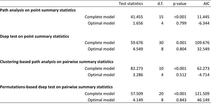
Table I-1: Path analysis and d-sep test statistics used to disentangle the effects of
environmental factors on allelic richness (point summary statistics) and genetic differentiation (pairwise summary statistics) using simplification procedures. ... 48
Table I-2: Estimates of the path coefficients of the optimal models and their associated
p-values and 95% confidence intervals (95% CI) obtained using path analysis. Clustering-based path analysis and permutation-based path analysis used on pairwise summary statistics provided similar p-values. ... 49
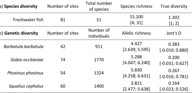
Table II-1: (a) Number of sites sampled, total number of species over all sites and mean and
range of species richness and true diversity; (b) number of sites and individuals sampled for all four species and mean and range of allelic richness and Jost's D. ... 85
Table II-2: General predictions (and underlying processes) regarding the relationships
between each latent variable and genetic and species diversity respectively. These predictions arise from general and local knowledge on the influence of each variable on genetic (Paz-Vinas et al. 2015) and species (Buisson et al. 2008; Blanchet et al. 2014) diversity... 88
Table II-3: Mean effect size (Ē), 95% confidence interval (95% CI), total heterogeneity of a
sample (Qt) and corresponding p-value (P) computed from the path coefficients obtained from
partial least-square path modeling applied to (a) α-diversity indices and (b) -diversity indices ... 96
Table III-1: General predictions (and underlying processes) regarding the influence of
environmental variables on intraspecidific α-diversity (a) and on intraspecidific -diversity. ... 126
Table III-2: D-sep test statistics used to disentangle the effects of environmental variables on
genetic and phenotypic α-diversity (a) and on genetic and phenotypic -diversity (b) in Gobio
occitaniae and Phoxinus phoxinus. For each species and diversity facet, we simplified a full
model (i.e. a model including all paths described in the main text) until reaching the models with the lowest AIC score represented in Figure III-5. ... 133
11 the best (ΔAIC < 4) linear mixed-effects models (one per relative warp and per species) linking relative warps to the environmental variables and their associated quadratic terms models ... 134
Table IV-1: Name, description and default value of the model main parameters. Fixed
parameters values were fixed over simulations. Parameters of interest were varied as described in the main text. ... 158
12
Liste des figures
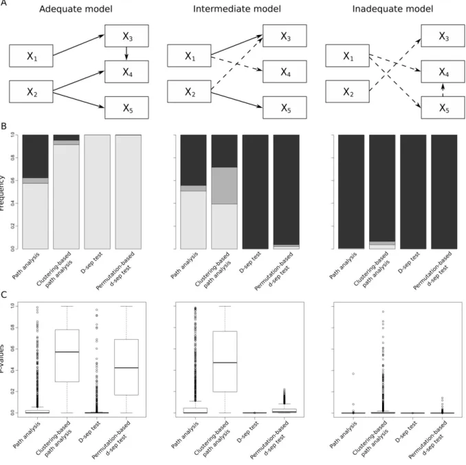
Figure I-1: A, Graphical representation of the “adequate”, “intermediate” and “inadequate”
models. B, Barplots summarizing the frequencies of ΔAIC values. C, Boxplots summarizing the p-values of both “adequate”, “intermediate” and “inadequate” models obtained over 1000 simulations with classical path analysis, clustering-based path analysis, the classical d-sep test and the permutation-based d-sep test.. ... 38
Figure I-2: A, Graphical representation of the model combining three “adequate” paths (black
arrows) and three “inadequate” paths (dotted arrows). B, Boxplots summarizing the p-values of the “adequate” and “inadequate” coefficients obtained over 1000 simulations with classical path analysis, clustering-based path analysis and permutation-based path analysis. ... 39
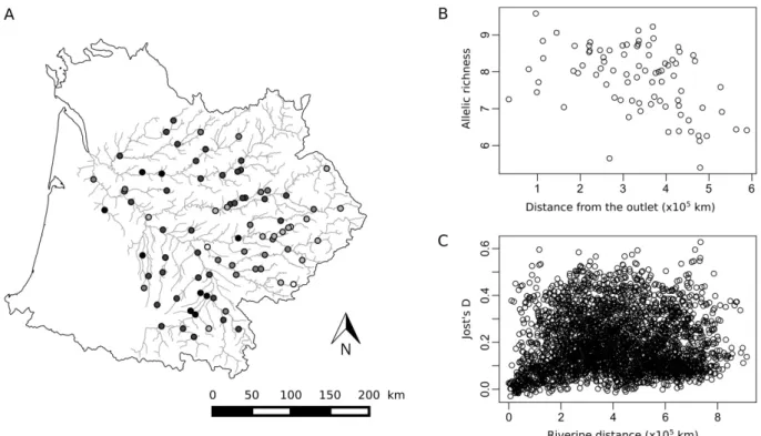
Figure I-3: Characteristics of genetic data. A, Location of the 83 sites, colored according to
their allelic richness. White: lowest values, black: highest values. B, Allelic richness plotted against distance from the outlet. C, Jost's D plotted against pairwise riverine distance. ... 42
Figure I-4: Graphical representations of A, the complete model depicting causal relationships
between allelic richness and anthropogenic and natural factors and B, the optimal model obtained after the simplification procedure.. ... 45
Figure I-5: Graphical representations of A, the complete model depicting causal relationships
between genetic differentiation and anthropogenic and natural factors and B, the optimal model obtained after the simplification procedure. ... 47
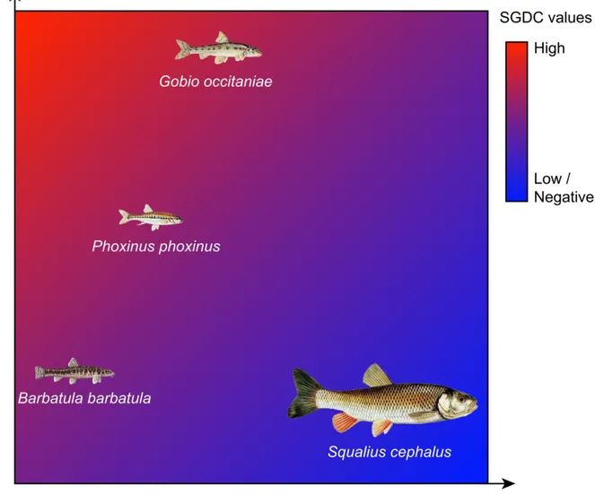
Figure II-1: Theoretical biplot showing how the strength of SGDCs is expected to vary
according to the rarity (y-axis) and the gene flow (x-axis) of the target species (i.e. the one used to quantify genetic diversity) and following theoretical works by Vellend (2005) and Laroche et al. (2015). ... 82
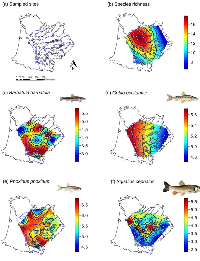
Figure II-2: Maps representing the spatial distribution of interpolated species richness (a) and
allelic richness of B. barbatula (b), G. occitaniae (c), P. phoxinus (d) and S. cephalus (e).. .. 90
Figure II-3: Allelic richness (genetic α-diversity) of B. barbatula (a), G. occitaniae (b), P.
phoxinus (c) and S. cephalus (d) plotted against species richness (species α-diversity) with
13
Figure II-4: Jost's D (genetic -diversity) of B. barbatula (a), G. occitaniae (b), P. phoxinus
(c) and S. cephalus (d) plotted against species richness (species -diversity) with Mantel's r and associated p-values. ... 93
Figure II-5: Graphical representation of the meta-analysis results obtained from Partial least
square path modeling on α-diversity indices over all species.. ... 94
Figure II-6: Graphical representation of the meta-analysis results obtained from Partial least
square path modeling on -diversity indices over all species. ... 95
Figure III-1: Location of the 48 sites sampled during summers 2014 and 2015 colored
according to the species present. ... 121
Figure III-2: Location of 16 homologous landmarks used to assess phenotypic diversity in Gobio occitaniae and Phoxinus phoxinus. ... 123
Figure III-3: Boxplots summarizing the genetic α-diversity (allelic richness) (a), phenotypic
α-diversity (proportion of shape space occupied by each population) (b), genetic -diversity (FST) (c) and phenotypic -diversity (euclidean distance between the consensus shapes of each pair of populations) (d) in Gobio occitaniae and Phoxinus phoxinus.. ... 130
Figure III-4: Genetic α-diversity (allelic richness) of Gobio occitaniae (a) and Phoxinus
phoxinus (b) plotted against phenotypic α-diversity (proportion of shape space occupied by each population) with Spearman’s rho and associated P-values; and genetic -diversity (Fst) of Gobio occitaniae (c) and Phoxinus phoxinus (d) plotted against -diversity (euclidean distance between the consensus shapes of each pair of populations) with Mantel’s r and associated P-values. ... 131
Figure III-5: Graphical representations of the models describing the causal relationships
between environmental variables and genetic and phenotypic α-diversity in Gobio occitaniae (a) and Phoxinus phoxinus (b), and between environmental variables and genetic and phenotypic -diversity in Gobio occitaniae (a) and Phoxinus phoxinus (b), obtained using the d-sep test.. ... 132
Figure IV-1: Spatial arrangement of the 36 habitat patches within the lattice configuration (a)
and the dendritic configuration (b). Dispersal is constraints along the network (grey lines).. ... 159
14
Figure IV-2: Mean maladaptation (a), partial correlation between phenotypical differentiation
and topographic distance after accounting for environmental difference (b) and partial correlation between phenotypical differentiation and environmental difference after accounting for topographic distance (c) obtained within the dendritic and the lattice configurations. ... 163
Figure IV-3: Mean maladaptation (a), correlation between maladaptation and betweenness
centrality (b), and correlation between maladaptation and distance from the river mouth (c) obtained within the dendritic configuration, with randomly-distributed habitat area and optimal phenotype, spatially-autocorrelated habitat area and randomly-distributed optimal phenotype, randomly-distributed habitat area and spatially-autocorrelated optimal phenotype and spatially-autocorrelated habitat area and optimal phenotype. ... 165
Figure IV-4: Partial correlation between phenotypical differentiation and topographic
distance after accounting for environmental difference (a) and partial correlation between phenotypical differentiation and environmental difference after accounting for topographic distance (b) obtained within the dendritic configuration ... 166
Figure IV-5: Mean maladaptation (a), correlation between maladaptation and betweenness
centrality (b), correlation between maladaptation and distance from the river mouth (c), partial correlation between phenotypical differentiation and topographic distance after accounting for environmental difference (d) and partial correlation between phenotypical differentiation and environmental difference after accounting for topographic distance (e) obtained within the dendritic configuration with spatially-distributed habitat area and optimal phenotype plotted in relation to the strength of gene flow and the migration range from upstream to downstream ... 167
15 “He floated on his back when the valise filled and sank; the river was mild and leisurely, going away from the people who ate shadows for breakfast and steam for lunch and vapors for supper. The river was very real; it held him confortably and gave him the time at last,
the leisure, to consider this month, this year, and a lifetime of years. He listened to his heart slow. His thoughts stopped rushing with his blood.” Ray Bradbury, Fahrenheit 451
16
Introduction
Biodiversity: a multifaceted concept experiencing critical loss
Biodiversity is a concept referring to the variability of life on the planet (Ricklefs and Miller 2000). According to the Convention on Biological Diversity signed by 165 countries during the Rio Earth Summit in June 199β, biodiversity “includes diversity within species, between species, and of ecosystems”.
Within-species diversity (hereafter named intraspecific diversity) is the most fundamental facet of biodiversity. It comprises genetic diversity (i.e. the diversity in the genetic information among individuals of a species) and phenotypic diversity (i.e. the diversity of behaviours, morphs and physiological traits among individuals of a species). Intraspecific diversity is the raw material on which acts selection, enabling species to adapt to environmental changes and ultimately leading to speciation (Ridley 2003). It improves species and communities resilience to disturbances (Jung et al. 2013; Moran et al. 2015). It plays a key role for evolutionary and ecological dynamics (Bolnick et al. 2003; Odling-Smee et al. 2003) by affecting the way species modulate their biotic and abiotic environment (Hughes et al. 2008; Bolnick et al. 2011).
Between-species diversity (hereafter named interspecific diversity) refers to the variety of species inhabiting an ecosystem and is the most obvious facet of biodiversity. Since the early 1990s, interspecific diversity has been hypothesized to positively influence ecosystem processes such as primary productivity, as well as their stability and maintenance in the face of disturbances (Loreau 2000a). Species richness (i.e. the number of species in an ecosystem) is extensively employed as a surrogate for interspecific diversity (Loreau 2010; Eduardo 2016) although functional complementarity among species is more and more acknowledged to have a greater impact on ecosystem functioning than species diversity per se (Eduardo 2016).
Finally, diversity of ecosystems refers to the number of different ecosystems on the planet. This notion accounts for the variety of unique ecological and evolutionary processes occurring in ecosystems such as interactions between species (predation, parasitism, coadaptation) and between species and their abiotic environment (primary production, nutrient cycling) (Begon et al. 2006).
17 Biodiversity can also be decomposed into three components: within-site diversity (α-diversity), between-site diversity ( -diversity) and the total regional diversity ( -diversity) (Whittaker 197β). As an example, at the intraspecific level, the α component of biodiversity is the diversity found within a population (e.g. the genetic diversity displayed by the individuals of a same population) whereas the component of biodiversity corresponds to the differentiation observed among populations (e.g. the genetic differentiation between two populations). Similarly, at the interspecific level, the α component of biodiversity is the diversity of species found within a community whereas the component of biodiversity is the difference of species composition among communities. The component of biodiversity describes the overall intraspecific or interspecific diversity of all the populations or communities of a region and has been defined as being the product ( = α × ; Whittaker 197β; Baselga β010) or the addition ( = α + ; Lande 1996; Loreau β000b) of the two other components.
All the facets of biodiversity are currently experiencing a dramatic decline caused by human actions (Butchart et al. 2010). This loss has been proven to directly affect ecological and evolutionary processes, thus reducing primary productivity and increasing ecosystems vulnerability to disturbances (Hooper et al. 2012). Additionally, the decrease in biodiversity has been shown to directly alter the benefits and services that humanity obtains from it, thus impacting human well-being (Díaz et al. 2006; Cardinale et al. 2012). In this context, the main challenge faced by scientists is to propose to decision-makers efficient and sustainable plans for limiting biodiversity loss. However, this requires an extensive understanding of the many facets and components of biodiversity, and notably of (i) how biodiversity is spatially distributed, (ii) what evolutionary and ecological processes shape the distribution of the facets and components of biodiversity and (iii) how the different facets of biodiversity interact with each other.
The patterns and drivers of biodiversity
Biodiversity is not evenly distributed on the planet (Gaston 2000). Some areas such as moist tropical forests harbour high biodiversity while others such as deserts are almost devoid of life. Studying this spatial distribution has allowed scientists to uncover repeated patterns
18
whereby biodiversity follows geographical or ecological gradients (Lawton 1996). For example, the most well defined and well known biodiversity pattern is the latitudinal gradient in interspecific diversity, i.e. the decrease of interspecific diversity from the equator to the poles (Pianka 1966). This pattern has been shown to hold true across many taxa, habitat types and geographic regions (Hillebrand 2004), and to affect both the α and the components of interspecific diversity (Willig et al. 2003). Another example is the species-area relationship, whereby species richness in an ecosystem tends to increase with the area of the ecosystem (Connor and McCoy 1979).
The underlying drivers of these patterns are complex and can stem from diverse evolutionary and ecological processes involving biotic and abiotic features. As an example, the latitudinal gradient in interspecific diversity has been hypothesized to result from higher rates of speciation in the tropics (Mittelbach et al. 2007), as well as from a variation in predation pressure promoting species coexistence (Freestone et al. 2011). For this reason, understanding the origins of biodiversity patterns is still an ongoing challenge. Nonetheless, it is also a fundamental goal of evolutionary biology and ecology (Levin 1992; Ricklefs 2004; Chave 2013) for several reasons. First, it allows to better understand the functioning of ecosystems at different spatial scales (Gotelli et al. 2009). Second, it gives the possibility to make predictions about the repartition of biodiversity across landscapes and about its response to environmental changes (Guisan and Thuiller 2005). Third, as stated above, it helps establishing efficient conservation measures through the identification of the most diverse areas and of the key features sustaining biodiversity.
Studying biodiversity patterns within integrative frameworks
Despite this critical importance, most of the biodiversity patterns described to this day relate to interspecific diversity, notably because it is one of the most convenient proxy measures of biodiversity (Maclaurin and Sterelny 2008). However, the other facets of biodiversity and notably intraspecific diversity ought not to be neglected as they are of critical importance for ecosystem functioning, stability and resilence (Blanchet et al. 2017; Mimura et al. 2017).
19 Studying each facet of biodiversity independently does not appear sensible. Indeed, it has long been acknowledged that inter- and intraspecific diversity were driven by parallel processes (i.e. speciation/mutation, ecological/genetic drift, dispersal/gene flow, environmental filtering/natural selection) possibly shaping them in comparable ways (Antonovics 1976). Consequently, it has been hypothesized that inter- and intraspecific diversity patterns might be similar and this result has been verified empirically (as an example, Adams and Hadly (2013) showed that, like interspecific diversity, intraspecific genetic diversity followed a latitudinal gradient in numerous vertebrate species). Additionally, similar patterns of inter- and intraspecific diversity could ensue from direct interactions between the two levels of biodiversity (Vellend and Geber 2005). For instance, a high interspecific diversity might generate diversifying selection in a population through disparate predation, thus increasing the intraspecific genetic diversity within this population.
In this context, studying in a single framework inter- and intraspecific biodiversity patterns, their drivers and the possible interactions between them appears crucial to test these fundamental hypotheses. To that aim, Vellend (2003) introduced the Species-Genetic Diversity Correlation concept (SGDC, see Chapter II) which quantifies the congruency in the patterns of interspecific diversity and intraspecific genetic diversity. The studies on SGDC led to a better understanding of the relationships between inter- and intraspecific genetic diversity, as well as the processes shaping these facets of biodiversity in similar or contrasting ways (Taberlet et al. 2012; Vellend et al. 2014).
Testing for parallel patterns in other facets of biodiversity appears of great interest. For instance, studying the correlation between genetic intraspecific diversity and phenotypic intraspecific diversity within a framework similar to SGDC seems judicious as these two facets of diversity are intrinsically related and can be under the influence of similar adaptive and neutral processes (Lowe et al. 2017). For instance, in the case of neutral genetic markers and adaptive traits that are not strongly affected by selection, genetic and phenotypic intraspecific diversity are expected to display similar patterns if they are driven by neutral processes such as drift. Direct relationships between genetic and phenotypic diversity can also be expected, notably when genetic diversity directly codes for the considered phenotypic traits or appropriately describes the whole genomic diversity (Hoffman et al. 2014). Therefore, these facets of biodiversity are expected to covary under specific conditions, and
20
uncovering similarities or dissimilarities in their distributions should ensure a better understanding of the underlying processes. To that aim, I developed a new concept named Genetic-Phenotypic Intraspecific Diversity Correlation (GPIDC, see Chapter III).
Such integrative frameworks appear essential to get an acute appraisal of the distribution of biodiversity on the planet. Additionally, knowing to what extend and under which conditions several facets of biodiversity might covary would favour the establishment of conservation measures targeting areas sustaining high diversity at the inter- and at the intraspecific level. However, describing biodiversity patterns and understanding what drives them is a major statistical challenge as it implies disentangling intricate causal relationships among numerous factors. This issue calls for the use of appropriate statistical approaches.
Causal modeling as a method to study biodiversity patterns
Most of the approaches used for linking biodiversity descriptors (e.g. species richness, allelic richness, etc.) to environmental variables rely on empirical correlations. However, as “correlation does not imply (direct) causation” (Shipley β000a), correlation provides no information on the underlying processes leading to the observed result. As an example, it is obvious that, even if a strong correlation is observed between latitude and biodiversity, latitude per se is not the direct cause of the latitudinal gradient in biodiversity. Consequently, the relations linking biodiversity descriptors to environmental variables have to be carefully interpreted, and may remain unexplained due to a statistical inability to tease apart causal relationships between variables (Shipley 2000a). Additionally, studying the patterns of several biodiversity facets in a single integrative framework such as SGDC calls for specific statistical approaches. Indeed, highlighting the environmental variables affecting two biodiversity descriptors while simultaneously testing for possible direct relationships between them requires statistical methods in which several dependent variables (here the biodiversity descriptors) can be taken into account simultaneously.
A solution to clarify entangled causal relationships within complex datasets may build on methods of causal modeling. Causal modeling assesses the validity of a model describing the expected causal links among a set of variables and estimates the strength of these links
21 (Grace 2006). Therefore, it allows to test for direct and indirect relations among diverse environmental variables and one or several biodiversity descriptors within a single framework. Two of the most used causal modeling approaches are maximum-likelihood based path analysis, initially introduced by Sewall Wright (1934) and the d-sep test developed by Bill Shipley (2000b). These methods are perfectly well suited to study biodiversity patterns at the α-level. However, at the -level, the variables are in the form of pairwise matrices (e.g. matrix of genetic differentiation among sites, see above). The statistical analysis of pairwise matrices poses a series of analytical issues, notably because of the non-independence of pairwise data (Legendre and Legendre 2012; Graves et al. 2013) that prevents the application of causal modeling. Consequently, the first chapter of the present work has been dedicated to the development of novel statistical approaches allowing the application of maximum-likelihood based path analysis and of the d-sep test to data in the form of pairwise matrices (see Chapter I). In the two subsequent chapters (Chapter II and III), I used causal modeling to uncover common patterns in three facets of biodiversity (namely interspecific diversity and intraspecific genetic diversity in Chapter II and intraspecific genetic diversity and intraspecific phenotypic diversity in Chapter III) in the particular context of riverine networks.
Biodiversity patterns in riverine networks
Freshwater habitats cover approximately 0.8% of the Earth’s surface but harbour 125,000 species of freshwater animals, representing 9.5% of all known animal species on the planet. This high concentration of biodiversity led some authors to define the entirety of freshwater habitats as a hotspot for biodiversity (Dudgeon et al. 2006; Strayer and Dudgeon 2010). This high interspecific diversity might be partially explained by the insular nature of freshwater habitats by which individuals are often restricted to a single biota (e.g. a lake or a river drainage), thus favouring speciation and endemism (Reyjol et al. 2007; Strayer and Dudgeon 2010). On the downside, the isolation between freshwater biotas impedes the ability of freshwater species to re-establish extinct populations and thus makes them very vulnerable to disturbances. Additionally, climate change is expected to strongly affect freshwater biodiversity (Heino et al. 2009) and human pressures on freshwater habitats are increasing, notably due to the rapid growth of the human population (Dudgeon et al. 2006).
22
Approximately 65% of all freshwater habitats have been declared to be under moderate to high threat due to human impacts such as water pollution, introduction of exotic species (e.g. Nile perch, water hyacinth, spinycheek crayfish) or flow modifications (Dudgeon et al. 2006; Vörösmarty et al. 2010). Remarkably, rivers are strongly impacted, with only an extremely small portion of the planet’s rivers remaining unaffected by humans (Vörösmarty et al. β010) while they harbour a high portion of the total freshwater biodiversity (Williams et al. 2004). Improving our understanding of the biodiversity patterns and drivers in riverine networks thus appears of critical importance to optimize their conservation.
Riverine networks are characterized by unique features. First, riverine networks harbour a distinctive dendritic structure (earning them the name of dendritic river networks, Fagan 2002; Grant et al. 2007) that consists of a mainstem to which are connected branches whose number typically increases from downstream to upstream. Second, riverine networks exhibit a strong upstream-downstream gradient of habitat capacities, with small physical carrying capacity in upstream branches (due to small river width) and larger carrying capacity in downstream branches and mainstems (larger river width). Third, riverine networks are characterized by an upstream-downstream gradient of environmental conditions. Upstream habitats are characterized by cold, highly oxygenated water, high water velocity, a coarse grain substrate and important vegetation cover while downstream habitats are characterized by warm and poorly oxygenated water, low water velocity, a fine grain substrate and scarce vegetation cover (Vannote et al. 1980).
Consequently, riverine networks are highly spatially-structured habitats, and biodiversity distribution is expected to highly contrast with what is observed within traditional two-dimensional landscapes (Altermatt 2013, see Chapter IV). The spatial connectivity of dendritic structures imposes huge dispersal constraints to freshwater species, especially in the case of species that can only disperse along the network (Grant et al. 2007, 2010). Notably, Carrara et al. (2012) experimentally showed a positive effect of dendritic structure on interspecific diversity. At the intraspecific level, Paz-Vinas and Blanchet (2015) theoretically demonstrated that dendritic configuration increased intraspecific genetic diversity when compared to two-dimensional lattice configuration. Additionally, migration in dendritic network is expected to be downstream-biased due to asymmetric dispersal costs caused by water flow and altitude (Morrissey and de Kerckhove 2009; Paz-Vinas et al. 2013) and the
23 combined effects of dendritic structure and asymmetric dispersal have been theoretically studied. For example, at the interspecific level, Muneepeerakul et al. (2008) found that interspecific -diversity was increased by asymmetric dispersal in dendritic networks while, at the intraspecific level, Morrissey and de Kerckhove (2009) showed that dendritic structure and asymmetric migration could maintain higher levels of intraspecific genetic diversity. The spatial structuring in habitat capacities is also expected to influence evolutionary and ecological processes in riverine networks. At the interspecific level, Carrara et al. (2014) found a positive effect of spatially-structured habitat sizes on the evenness of community composition within a theoretical dendritic network when compared to randomly distributed or uniform habitat sizes. At the intraspecific level, Paz-Vinas et al. (2015) showed that the increase in habitat capacity downstream could generate an increase in genetic diversity. The impact of the environmental gradient on biodiversity has also been studied, mainly empirically. Notably, at the interspecific level, species assemblages are known to greatly vary along this gradient (Vannote et al. 1980; Schlosser 1990) and similarly, at the intraspecific level, individual phenotypes have been shown to follow this gradient (e.g. Hopper et al. 2015). These variations are expected to lead to high inter- and intraspecific -diversity within riverine networks.
Disentangling the relative impacts of these features on biodiversity distribution appears challenging but is essential to the understanding and optimal protection of riverine networks. In complement to the empirical studies presented in Chapters II and III, I chose to use an eco-evolutionary model to theoretically solve this issue (Chapter IV).
Objectives
The main objective of the present work has been to study the patterns of inter- and intraspecific diversity within riverine networks. More specifically, I aimed at uncovering if interspecific diversity, intraspecific genetic diversity and intraspecific phenotypic diversity were similarly distributed, at both the α and the levels. Additionally, I investigated which features of the riverine networks shaped interspecific diversity, intraspecific genetic diversity and intraspecific phenotypic diversity. This was achieved empirically through the use of integrative frameworks and theoretically through the use of an eco-evolutionary metapopulation dynamics model (Hanski et al. 2011).
24
This thesis has been divided into four chapters.
The first chapter has been dedicated to the development of statistical approaches allowing the application of causal modeling methods (namely path analysis and the d-sep test) to data in the form of pairwise matrices, in order to study biodiversity patterns and their underlying processes at the α and levels within similar statistical frameworks.
In the second chapter, I studied the similarities and dissimilarities between interspecific diversity and intraspecific neutral genetic diversity patterns in four freshwater fish species (namely Barbatula barbatula, Gobio occitaniae, Phoxinus phoxinus and Squalius
cephalus) within the Garonne-Dordogne riverine network. I investigated the causes of these
patterns using an integrative framework (namely the SGDC framework, Vellend and Geber 2005) in order to uncover the processes underlying the spatial distribution of inter- and intraspecific diversity while taking into account the possible interactions between them.
In the third chapter, I tested for congruencies between the distributions of intraspecific neutral genetic diversity and intraspecific phenotypic diversity in two freshwater fish species (namely G. occitaniae and P. phoxinus) within the Garonne-Dordogne riverine network. I again used an integrative framework (named GPIDC) to uncover the drivers of these two facets of intraspecific diversity and the possible interactions between.
In the fourth and last chapter of this thesis, I used an eco-evolutionary metapopulation dynamics model to theoretically assess the impacts of the main features of riverine networks (i.e. the dendritic structure, the upstream-downstream gradient in habitat capacities, the upstream-downstream gradient in environmental conditions and the asymmetric dispersal rate caused by water flow) on local adaptation and on the distribution of intraspecific phenotypic diversity.
25
Chapter I - Inferring causalities in landscape genetics: An
extension of Wright's causal modeling to distance matrices.
By Lisa Fourtune1, Jérôme Prunier1, Ivan Paz-Vinas2,3,4, Géraldine Loot1,5, Charlotte Veyssière5 and Simon Blanchet1,4
1 Centre National de la Recherche Scientifique (CNRS), Université Paul Sabatier (UPS); UMR 5γβ1 (Station d’Écologie Théorique et Expérimentale, SETE), 09200 Moulis, France 2 Aix-Marseille Université, CNRS, Institut de Recherche pour le Développement (IRD), Avignon Université; UMR 7263 (Institut Méditerranéen de la Biodiversité et d'Ecologie marine et continentale, IMBE), Centre Saint-Charles, Case 36, Marseille, France
3 Université de Lyon, CNRS, École nationale des travaux publics de l'Etat (ENTPE); UMR 5023 (Laboratoire d'Ecologie des Hydrosystèmes Naturels et Anthropisés, LEHNA), 6 rue Raphaël Dubois, 69622 Villeurbanne, France
4 CNRS, UPS, École Nationale de Formation Agronomique (ENFA); UMR 5174 (Laboratoire Évolution & Diversité Biologique, EDB), 31062 Toulouse cedex 4, France
5 Université de Toulouse, UPS; UMR 5174 (EDB), 31062 Toulouse cedex 4, France
26
I.1 - Résumé
Identifier les caractéristiques du paysage qui affectent la connectivité fonctionnelle entre populations est un défi crucial tant pour l’écologie fondamentale qu’appliquée. La génétique du paysage combine des données génétiques et écopaysagères afin de résoudre cette problématique, et doit pour cela identifier les relations directes et indirectes existant au sein de jeux de données complexes. Le recours aux outils d’analyses causales (« causal modeling ») apparait dans ce contexte comme particulièrement adapté. Néanmoins, cette approche statistique n’a pas été initialement développée pour être appliquée à des données prenant la forme de matrices de distance, comme c’est souvent le cas en génétique du paysage. Dans cette étude, notre objectif est d’étendre le domaine d’application de deux méthodes d’analyses causales (le path analysis et le d-sep test) en développant des approches statistiques adaptées aux matrices de distances. Grâce à des simulations, nous avons démontré que ces nouvelles approches amélioraient grandement la robustesse des ces méthodes. A partir d’un jeu de données empiriques combinant des données génétiques d’une espèce de poisson d’eau douce (Gobio occitaniae) et des données écopaysagères, nous avons démontré l’intérêt des analyses causales pour mieux connaitre la connectivité fonctionnelle au sein de populations sauvages. Nous avons notamment démontré que des relations directes et indirectes impliquant l’altitude, la température et la concentration en oxygène de l’eau influençaient la diversité génétique inter- et intra-populationnelle chez G. occitaniae.
27
I.2 - Abstract
Identifying landscape features that affect functional connectivity among populations is a major challenge in fundamental and applied sciences. Landscape genetics combines landscape and genetic data to address this issue, with the main objective of disentangling direct and indirect relationships among an intricate set of variables. Causal modeling has strong potential to address the complex nature of landscape genetic datasets. However, this statistical approach was not initially developed to address the pairwise distance matrices commonly used in landscape genetics. Here, we aimed to extend the applicability of two causal modeling methods, i.e., maximum-likelihood path analysis and the directional-separation test, by developing statistical approaches aimed at handling distance matrices and improving functional connectivity inference. Using simulations, we showed that these approaches greatly improved the robustness of the absolute (using a frequentist approach) and relative (using an information-theoretic approach) fit of the tested models. We used an empirical dataset combining genetic information on a freshwater fish species (Gobio
occitaniae) and detailed landscape descriptors to demonstrate the usefulness of causal
modeling to identify functional connectivity in wild populations. Specifically, we demonstrated how direct and indirect relationships involving altitude, temperature and oxygen concentration influenced within- and between-population genetic diversity of G. occitaniae.
28
I.3 - Introduction
Landscape genetics is a discipline aimed at understanding spatial patterns of genetic diversity by exploring the relationships between landscape features and microevolutionary processes such as genetic drift, selection, mutation and gene flow (Manel et al. 2003; Manel and Holderegger 2013). This discipline builds on the latest advances in molecular biology and landscape data processing and is becoming increasingly important for fundamental and applied sciences (Storfer et al. 2010; Keller et al. 2015). Landscape genetics addresses issues ranging from the identification of barriers to dispersal, to the inference of the spread of non-native species (Storfer et al. 2010).
The main objectives of landscape genetics are to spatially describe effective dispersal (i.e., gene flow) and to identify landscape features (e.g., roads, dams, urban areas, and rivers) that affect functional connectivity (Manel et al. 2003; Storfer et al. 2010; Manel and Holderegger 2013). To achieve these objectives, landscape geneticists calculate genetic descriptors that are subsequently compared with landscape features and potential dispersal barriers (Balkenhol et al. 2009; Jaquiéry et al. 2011; Bradburd et al. 2013). Analytical tools developed for analyzing landscape genetic data often rely on empirical correlations that allow an assessment of the possible influence of various evolutionary processes. For example, a significant and positive correlation between genetic and geographic distances is generally considered indicative of isolation-by-distance (IBD: a spatial pattern whereby the homogenizing effect of gene flow decreases and the relative effect of genetic drift increases as the geographic distance between sites increases; Hutchison and Templeton 1999).
However, because “correlation does not imply causation”, processes can be incorrectly inferred from empirical correlations (Guillot et al. 2009). The likelihood of incorrectly inferring causalities from correlation is exacerbated in landscape genetics because it often implies intricate relationships among landscape variables. In the IBD example described above, the correlation between genetic and geographic distances might be direct, indirect and/or spurious. The correlation is “direct” (i.e., the migration rate between two sites decreases because they are far from one another) if no other variable co-varying with geographic distances causes the observed pattern of genetic distance. However, if a variable co-varies with geographic distances (e.g., the number of barriers between two sites) and causes the observed pattern, then the correlation between genetic and geographic distances is “indirect”. Alternatively a correlation is “spurious” when two variables are correlated because
29 they are both influenced by a third (unmeasured) variable (Cushman and Landguth 2010; Prunier et al. 2015). In the two latter cases, processes are incorrectly inferred from simple correlations. Consequently, the relationships linking landscape features to genetic descriptors have to be carefully interpreted, and they sometimes remain unexplained due to our inability to disentangle intricate relationships between variables (Shipley 2000a; Grace 2006). Clarifying causal relationships in landscape genetics is thus challenging, but important (Guillot et al. 2009).
A solution to improve inferences of causal relationships in landscape genetics may build on methods of causal modeling (e.g., Cushman et al. 2006). Causal modeling procedures, such as path analysis (Grace 2006), rely on the assessment of the validity of a causal graph describing the expected direct and indirect causal relationships among variables. Path analysis was initially developed by one of the founding fathers of population genetics, namely, Sewall Wright (1921). In path analysis, the influence along each path of the causal graph (i.e., the link between two variables) is estimated from correlation/covariance among the involved variables. Almost a century after its introduction by one of the most influential population geneticists, and despite its relevance for analyzing complex observational data, path analysis is still only occasionally used in landscape genetics and in population genetics in general.
Landscape geneticists generally focus on two main types of dependent variables that describe genetic diversity: (i) point summary statistics, which describe the genetic diversity at the sampling site level (e.g., allelic richness or heterozygosity) and (ii) pairwise summary statistics, which describe the genetic differentiation (or distance) between pairs of sampled populations or individuals (e.g., Fst, Jost's D). Several well-established methods allow a straightforward analysis of point summary statistics in a path analysis framework (Shipley 2000a; Grace 2006). For pairwise statistics, however, the process is more complex since the analysis of pairwise matrices poses a series of analytical issues, notably because of the non-independence of pairwise data (Legendre and Legendre 2012; Graves et al. 2013). Although pairwise data can be handled by reducing multidimensionality, using NMDS or dbRDA, for instance (e.g., Legendre and Fortin 2010), these types of analyses were not developed to tease apart direct and indirect relationships and are more suited to answer questions involving dissimilarity matrices rather than distance matrices (Legendre and Fortin 2010; Legendre et al. 2015). To address this specific data type, Cushman et al. (2006, 2013) proposed a causal modeling procedure based on partial Mantel tests to compare several competing causal models that link a matrix of genetic distances to matrices of explanatory variables. This
30
approach permits an assessment of the goodness-of-fit of each model by independently comparing the observed results of partial Mantel tests (partial correlation coefficients and associated p-values) to what is theoretically expected under each model specification. This approach has been proven to be powerful for inferring causalities from relatively simple models (Cushman and Landguth 2010). However, the design of the causal graph is constrained by the number of matrices of explanatory variables that can be handled in partial Mantel tests (only two), which limits the complexity of competing models and prevents the assessment of indirect relationships among variables. We believe that the use of alternative causal modeling procedures, such as maximum-likelihood-based path analysis (hereafter called “path analysis” for the sake of simplicity) and the directional-separation test (hereafter called “d-sep test”, Shipley β000a, 2000b), can represent an interesting improvement over the approach proposed by Cushman et al. (2006), as they may simultaneously account for all correlations implied in a model and permit the design (and comparison) of more complex models, explicitly addressing both direct and indirect effects.
We propose a simple and integrative framework to study direct and indirect links in the context of the analysis of landscape genetic data (and more generally, of ecological and evolutionary data involving pairwise matrices). As an introduction, we briefly present the philosophy, advantages and disadvantages of path analysis and the d-sep test. Then, we extend the applicability of these two methods to pairwise matrices (including distance and dissimilarity matrices) by developing two statistical approaches aimed at analyzing complex causal models (i.e., including several pairwise matrices linked both directly and indirectly) in landscape genetics. We then test the robustness of path analysis and the d-sep test applied to pairwise matrices using simulations. Finally, we use an empirical dataset involving patterns of genetic diversity in a freshwater fish species (Gobio occitaniae) and landscape descriptors at the river basin scale to demonstrate how these two statistical procedures can be used in landscape genetics to answer important biological questions. This study provides an opportunity to reconcile two important legacies of Sewall Wright's scientific life: population genetics and path analysis.
31
I.4 - A brief description of path analysis and the d-sep test
An introduction to causal graphs
Any causal modeling procedure is based on a causal graph illustrating the a priori hypotheses underlying the potential causal relationships within a set of variables. These relationships are depicted by vertices (i.e., nodes) representing variables that are linked by edges. A causal graph can contain manifest variables that are directly observed and measured (Shipley 2000a); error variables, which represent all of the factors that are not considered in the current graph; and latent variables that are hypothesized to exist but have not been measured directly (Grace 2006). Causal graphs are an intuitive approach to translate a causal hypothesis into a statistical language. The next step is to statistically test the relevance of the causal model in relation to data. Here, we focused on path analysis and the d-sep test, two methods dedicated to testing causal models without latent variables (Shipley 2000a; Grace 2006). These two methods are described below. When the causal graphs contain latent variables, the dedicated method is called structural equation modeling (SEM; Grace 2006), which is a generalization of path analysis. This method will not be presented here.
Path analysis
Path analysis is based on maximum likelihood estimation (Fisher 1950) of model parameters through the computation of covariance matrices. Each causal model includes a set of parameters, some of which are known (e.g., variances and covariances of variables), whereas others are unknown (e.g., path coefficients that quantify the direct influence of a variable along a given path; Wright 1921). The first step is to infer values for these unknown parameters. This inference is made iteratively by computing a maximum likelihood fitting function (FML; Bollen 1989) that quantifies the difference between the observed covariance
matrix and a covariance matrix computed using the inferred values. The best parameter values are those that minimize this function. The absolute fit of the model can be assessed by computing a chi-square statistic and an associated p-value to determine whether the minimal value of FML is small enough to conclude that the observed data fit the hypothesized causal
model; a high p-value indicates a high probability that the observed data fit the hypothesized causal model. Additionally, the relative fit of competing models can be tested using an information-theoretic approach (e.g., using Akaike's Information Criterion, AIC; Bollen 1989).