HAL Id: hal-01987902
https://hal.laas.fr/hal-01987902
Submitted on 21 Jan 2019
HAL is a multi-disciplinary open access
archive for the deposit and dissemination of
sci-entific research documents, whether they are
pub-lished or not. The documents may come from
teaching and research institutions in France or
abroad, or from public or private research centers.
L’archive ouverte pluridisciplinaire HAL, est
destinée au dépôt et à la diffusion de documents
scientifiques de niveau recherche, publiés ou non,
émanant des établissements d’enseignement et de
recherche français ou étrangers, des laboratoires
publics ou privés.
Geometric algorithms for the conformational analysis of
long protein loops
Juan Cortés, Thierry Simeon, Magali Remaud Simeon, V. Tran
To cite this version:
Juan Cortés, Thierry Simeon, Magali Remaud Simeon, V. Tran. Geometric algorithms for the
con-formational analysis of long protein loops. Journal of Computational Chemistry, Wiley, 2004, 25 (7),
pp.956-967. �10.1002/jcc.20021�. �hal-01987902�
Geometric
Algorithms for the Conformational Analysis of
Long
Protein Loops
J. CORTE´ S,1 T. SIME´ ON,1 M. REMAUD-SIME´ ON,2 V. TRAN3
1
LAAS-CNRS, 7 avenue du Colonel-Roche, 31077 Toulouse, France 2
Centre de Bioingenierie Gilbert Durand, 135 avenue de Rangueil, 31077 Toulouse, France 3
Unite´ de Recherches sur la Biocatalyse, 2 rue de la Houssinie`re, 44322 Nantes, France
Abstract: The efficient filtering of unfeasible conformations would considerably benefit the exploration of the conformational space when searching for minimum energy structures or during molecular simulation. The most important conditions for filtering are the maintenance of molecular chain integrity and the avoidance of steric clashes. These conditions can be seen as geometric constraints on a molecular model. In this article, we discuss how techniques issued from recent research in robotics can be applied to this filtering. Two complementary techniques are presented: one for conformational sampling and another for computing conformational changes satisfying such geometric constraints. The main interest of the proposed techniques is their application to the structural analysis of long protein loops. First experimental results demonstrate the efficacy of the approach for studying the mobility of loop 7 in amylosucrase from Neisseria polysaccharea. The supposed motions of this 17-residue loop would play an important role in the activity of this enzyme.
Key words: conformational search; robotic motion planning; loop closure; steric clash avoidance; long protein loops
Introduction
Prime techniques in structural investigations require the explora-tion of the conformaexplora-tional spaceᏯ of a molecule. Conformational search methods1
explore Ꮿ to identify the stable structures of molecules, which determine their properties and functions. Molec-ular simulations2
explore Ꮿ while computing conformational
changes on a molecule under modified environmental conditions. The analysis of such changes of the molecular structure is essential for the understanding of many biologic processes.
Because the goal of the conformational search is to find min-imum energy structures, the exploration is much more efficient when it is limited to a subset ofᏯ excluding energetically unac-ceptable conformations. Conformational changes explored in sim-ulations can occur only if there is not a high energetic barrier to overcome. Therefore, approaches treating these problems will greatly benefit from efficient techniques able to provide samples and paths inᏯ that filter most unfeasible conformations.
The conformational analysis of a whole macromolecule is a difficult problem. From a methodological point of view, two stages are usually necessary: the first corresponds to the identification of rigid segments (i.e., secondary structural elements) capable of participating in the molecular framework; the second is devoted to the remaining segments, so-called loops, assumed to be much
more flexible. However, available techniques to predict low-en-ergy conformations of long loops are limited and much less effi-cient because of the loop flexibility.
When the global molecular architecture is assumed to be known and only portions (loops) are studied separately, the integ-rity of molecular chains must be maintained. The first and last atoms of the treated segment of a molecular chain must remain bonded with their neighbor atoms. Breaking these bonds requires a high amount of energy. A strong constraint is thus imposed for the conformational exploration. This same constraint is present in the analysis of cyclic molecules. It is often referred to in the literature as the loop-closure constraint. Three main kinds of methods can be applied to solve the loop-closing problem (i.e., computing conformations satisfying loop closure): analytic (e.g., refs. 3–5), optimization-based (e.g., refs. 6 – 8), and database meth-ods (e.g., refs. 9 and 10). The difficulty of this problem increases with the length of the molecular chain, and available techniques are limited, or at least strongly penalized, by this.
In addition to breaking bonds, another large amount of energy is required to get two nonbonded atoms significantly closer than the sum of their van der Waals (vdW) radii. A violation of this condition is called steric clash. Feasible conformations of a
mo-lecular segment cannot contain either internal clashes, which we call self-clashes, or clashes with atoms of the rest of the molecule. A possible filter for such unacceptable conformations consists of evaluating the repulsive term of the vdW energy and discarding conformations that exceed a given cutoff value.11
However, this energetic constraint can also be treated by geometric procedures. The use of “clash grids,” computed from the distances between atoms, to perform this filtering was proposed in ref. 12. An interesting alternative is the use of collision detection algorithms applied on a 3D model of the molecule.13Obviously, the higher
the number of atoms the more critical the efficiency of the tech-nique.
In robotics, the same kinds of constraint appear when treating the motion planning problem.14
Paths must be computed in the subset of feasible configurations* of the robot, Ꮿfeas. The main
feasibility condition is collision avoidance. The robot cannot col-lide with obstacles in the workspace and self-collisions are also forbidden. Besides, when the robotic mechanism contains kine-matic loops closure constraints must be considered in the com-puted motions. Sampling-based motion planning techniques (e.g., refs. 15–17) have been demonstrated to be efficient and general tools in this field. These techniques capture the topology ofᏯfeas
within data structures (graphs or trees) by performing a random (or quasirandom) exploration of Ꮿ on a model of the robot and its environment.
In recent publications,18,19
we described efficient algorithms for planning motions of closed-chain mechanisms. In this article, we investigate the adaptation of these techniques to handle mo-lecular models. Although the method could be applied to any molecular segment or cyclic molecule, we are mainly interested in the application to long protein loops.
Interest in Protein Loops
Loops play key roles in the function of proteins. They are often involved in active and binding sites. Therefore, when predicting a protein structure an accurate loop modeling is necessary for de-termining its functional specificity.
Modeling loops in proteins is one of the main open problems in structural biology. Comparative modeling methods (see ref. 20 for a survey) often fail in the prediction of protein loop structures when the percentage of sequence identities between known and predicted protein family members is low. Indeed, it is well estab-lished that there is no reliable approach for modeling long loops (more than five residues) available at this time.21
The alternatives to comparative modeling are de novo (or ab
initio) methods.22
Such methods carry out a search of low-energy conformations for a given amino acid sequence. Many different approaches have been proposed for modeling protein loops. One of the most developed techniques is described in ref. 23. This refer-ence article also provides a concise survey of loop modeling methods. The accuracy of de novo methods mainly depends on the
energy function they use. Therefore, improvements in the results provided by these approaches require the design of fine-energy models. However, progress in the conformational exploration strategies may also be necessary to increase the efficiency of these techniques, which are today computationally expensive.
Even more important than the prediction of stable loop confor-mations is the determination of the feasible conformational changes. In many enzymes, for example, surface loops undergo conformational changes to catalyze a reaction.24
Further, loop motions are in general involved in protein interactions. Therefore, introducing loop flexibility into docking approaches is necessary for a more accurate prediction of these interactions.25
Aim of Our Approach
The techniques proposed in this article aim to be new tools for the structural analysis of long polypeptide segments and, in particular, of protein loops. The efficiency of geometric algorithms developed in the field of robotics can relieve conformational exploration approaches of a part of the heavy energetic treatment.
In Section 5, we propose a conformational sampling technique that generates random conformations satisfying loop-closure and clash avoidance constraints. The backbone conformation is first computed by an algorithm that relies on efficient geometric and kinematic procedures. Side-chain conformations are then gener-ated by combining sampling techniques and an effective collision detection algorithm. Families of approaches requiring conforma-tional sampling, such as Monte Carlo algorithms26
or stochastic roadmap techniques,27
would directly benefit from such filtered conformations.
Another interesting feature of our sampling technique is to compute loop conformations avoiding steric clashes with the rest of the protein. Using this technique to compute random samples uniformly distributed in the conformational space will provide useful information about the allowed conformations of the loop in its environment. For instance, this information could be repre-sented in the form of Ramachandran plots,28
and techniques (e.g., MODELLER23) using such statistical distributions could gain in
performance.
The geometric analysis can be pushed further. In Section 6, we propose an algorithm to capture the connectivity of the subspace of geometrically feasible conformations. The possible deformations maintaining loop-closure and clash avoidance constraints are ex-plored and encoded in a data structure. Such a data structure would be useful for many existing conformational exploration ap-proaches. Note that a conformational search method sharing sim-ilar ideas has been proposed in ref. 29 for small molecules (li-gands) under geometric constraints.
Problem Formulation
The problem is formulated from a robotic point of view. First, the geometric model of the molecule is described. The constraints that must be satisfied during the exploration of the conformational space are then defined.
*A configuration for a robot is equivalent to a conformation for a molecule. We designate both, the configuration space and the conformational space, byᏯ.
Geometric Model
Kinematics-Inspired Model
A molecule is a set of atomsᏭipartially connected by bonds. A
sequence of bonded atoms is called a molecular chain. Three parameters, usually called internal coordinates, define the relative position of consecutive atoms in a molecular chain: bond lengths, bond angles, and dihedral angles. The widely adopted rigid
geom-etry assumption (see ref. 30 as one of the first references) considers
that only dihedral angles are variable parameters. Under this as-sumption, a molecule can be seen as an articulated mechanism with revolute joints between bonded atoms. The model of a mo-lecular chain can be built from the internal coordinates using kinematics conventions. We follow the modified
Denavit–Harten-berg (mDH) convention described in ref. 31. A Cartesian
coordi-nate system Fiis attached to each atomᏭiand then the relative
location of consecutive frames can be defined by a homogeneous transformation matrix: i⫺1T i⫽
冢
Ci ⫺Si 0 0 SiC␣i⫺1 CiC␣i⫺1 ⫺S␣i⫺1 ⫺S␣i⫺1di SiS␣i⫺1 CiS␣i⫺1 C␣i⫺1 C␣i⫺1di 0 0 0 1冣
where diis the bond length between atomsᏭi⫺1andᏭi;␣i⫺1is
the supplement of the bond angle betweenᏭi⫺2,Ꮽi⫺1, andᏭi;
iis the dihedral angle formed by atoms Ꮽi⫺2, Ꮽi⫺1, Ꮽi, and
Ꮽi⫹1[see Fig. 1(a)]. C and S represent sines and cosines,
respec-tively.
A molecular chain between atomsᏭ0andᏭnis then modeled by
a kinematic chain,1
n, in which joint variables correspond to dihedral
angles. The conformation of the chain is determined by the array q of thei. The kinematic model of a polypeptide segment is composed of
a set of chains: the main-chain (the backbone) and the side-chains,
which are built upon it. The conformation of the segment is then specified by an array containing the conformation parameters of the backbone and of all the side-chains.
Often, some portions of molecular models are treated as rigid solids, for instance, peptide units in proteins. The rigid geometry assumption also considers that double-bond torsion angles, such as peptide bonds, are fixed. Hence, the number of frames required in the kinematic modeling is reduced. Figure 1(b) illustrates how the frames corresponding to the mDH parameters are obtained by simple geo-metric operations when the dihedral angle associated with a peptide bond is fixed at a given value. Thus, several atoms in each peptide unit have constant coordinates in these frames. As proposed in a recent work,32
frames only need to be attached to rigid units (called
atomgroups by the authors). Then, the relative location of atoms in an
atomgroup only requires positional coordinates, yielding to a more efficient method for updating conformations.
vdW Model
The vdW model consists of a representation of the molecule by the union of solid spheres associated with atoms. A vdW radius is assigned to each atom type. This geometric model of the molecule is the simplest and most ordinary space-filling diagram.33
In mo-lecular models treated by our approach, such spheres are the mobile bodies of the articulated polypeptide segment and the static
obstacles corresponding to the rest of the atoms in the molecule,
which compose what we call the environment.
Geometric Constraints
Loop Closure
A loop-closure constraint applied on the kinematic model of a molecular chain1
n fixes the relative location of the frames F0
and Fn, which we call base-frame and end-frame, respectively. Figure 1. Molecular chain model. Frames associated (a) with atoms and (b)
defining the articulated mechanism. [Color figure can be viewed in the online issue, which is available at www.interscience.wiley.com.]
Therefore, the transform matrix0
Tnis known. This matrix can also
be obtained from the sequence of local transformations:
0 Tn⫽ 0 T1 1 T2. . . n⫺1T n
This equality provides a system of equations, called closure
equa-tions, where the unknowns are the joint variables i. Hence, a
relationship must exist between the parameters in q for satisfying loop closure.
Clash Avoidance
Distances between nonbonded atoms that are substantially shorter than the sum of their vdW radii must be avoided. The choice of the limiting contact distance is ambiguous. For our experiments, we model molecules using a percentage (usually 70%) of the vdW radii proposed in ref. 34. Collisions between such reduced vdW spheres must be avoided if they are separated by more than three bonds. This condition must be satisfied between the atoms of the articulated segment and between these atoms and the static atoms of the rest of the molecule.
Conformational Sampling
Algorithm 1 computes a random conformation of a polypeptide segment (the protein loop) achieving loop-closure and clash avoid-ance constraints on the 3D model. First, the backbone conforma-tion qbis generated. The procedure for obtaining random
confor-mations satisfying closure is explained in the next subsection. These conformations are then tested for clashes of backbone atoms between themselves and with atoms in the environment. Once a feasible conformation for the backbone has been computed, ran-dom conformations of the side-chains qsare tested. These chains
are built iteratively until all of them are free of clashes. The process is explained below.
Backbone Conformation with Closure
Obtaining a backbone conformation satisfying loop closure re-quires the solution of the closure equations mentioned above. Unfortunately, and despite the intensive research in the field, no
efficient general solution is currently available to solve systems of multivariable nonlinear algebraic equations (see ref. 35 for a survey).
It is now well known that, in general, six variables in the closure equations are dependent on the rest (independent vari-ables). Note that six is the minimum number of parameters that allow us to span full-rank subsets of SE(3) (the position-orienta-tion space in a 3D world).14
Many articles in computational chemistry and robotics (e.g., refs. 3, 5, and 36 –39]) propose methods to obtain these six dependent variables as a function of the other parameters. Except for very particular geometries (e.g. regular cyclohexane40
), only a finite number of solutions exists. The remaining difficulty is how to obtain values for the inde-pendent variables for which a solution of the closure equations exists. In robotics, detailed analytic approaches have been pro-posed only for planar or spherical closed mechanisms.41
In com-putational chemistry, only a few authors have tackled this problem. Decimation approaches and hierarchical decomposition of the closing problem have been proposed for loops with six or more residues.5
However, for very long loops the efficiency of such methods decreases because closure equations must be solved sev-eral times for different fragments of the chain.
We propose an algorithm, called random loop generator (RLG), that produces random configurations of articulated mech-anisms containing closed chains. This algorithm has demonstrated its efficiency within robotic motion planning techniques.18,19The
configuration parameters of a closed kinematic chain are separated into two arrays: we call the independent variables of the closure equations the active variables qa
and the dependent variables the
passive variables qp. The RLG algorithm performs a particular
random sampling for qa
that notably increases the probability of obtaining solutions for qp
.
We next explain the main elements of our approach and how it can be applied to polypeptide backbone segments. Explanations are illustrated on a simple mechanism, the 6R planar linkage in Figure 2. Theᏸiare the rigid bodies and the Jithe revolute joints
connecting them.
Loop Decomposition
The choice of the dependent and independent variables in the closure equations is arbitrary. We choose them consecutively in the kinematic chain. Thus, we can refer to a passive subchain involving joints whose variables are in qp
(passive joints). Al-though the passive subchain can be placed anywhere in the closed chain, it is convenient to place it in the middle. In general, the passive subchain is a mechanism with six degrees of freedom. For a polypeptide backbone model under the rigid geometry assump-tion, only dihedral angles and are variable. Therefore, the passive subchain is composed of the backbone of three residues. In the example in Figure 2, three consecutive revolute joints (i.e., a 3R planar mechanism) are sufficient. We have chosen J3, J4, and
J5to be the passive joints of the 6R linkage. Then, the rest of the
joints (active joints corresponding to qa
) can be seen as contained in two active subchains rooted on the (fictive) solid on which the base frame and the end frame are fixed (ᏸ0,6in Fig. 2).
Algorithm 1: RANDOMLOOPCONF.
input : the loop, the rest of the protein
output : the conformation q
begin
qb4 RANDOMBACKBONECONF(loop.bkb); if not CLASHCHECK(qb, loop.bkb, protein) then
if qs4 GENERATESIDECHAINS(qb, loop, protein) then q4 COMPOUNDCONF(loop, qb, qs);
else return Failure; else return Failure; end
RLG Algorithm
The pseudocode of the algorithm that generates random configu-rations of a single-loop closed chain (applied to the loop backbone) is synthesized in Algorithm 2. First, the configuration parameters of the active subchains, qa
, are computed by the function SAM
-PLE_qa detailed in Algorithm 3. The idea of the algorithm is to
progressively decrease the complexity of the closed chain treated at each iteration until only the configuration of the passive sub-chain, qp
, remains to be solved. The two active subchains are treated alternately. The ideal solution should be to sample each
joint variable from the subset of values, which we call closure
range, satisfying the closure equations. However, computing this
subset is as difficult as solving the general closure equations. Thus, an approximation is used. This approximation must be conserva-tive to guarantee a complete solution (i.e., no region of the sub-space satisfying closure constraints is excluded from the
sam-Figure 2. Steps of the RLG algorithm performed on a 6R planar linkage. [Color figure
can be viewed in the online issue, which is available at www.interscience.wiley.com.]
Algorithm 2: RANDOMBACKBONECONF.
input : the backbone
output : the conformation qb begin
qa4 SAMPLE_qa(backbone); if qp4 C
OMPUTE_qp(backbone, qa) then qb4 COMPOUNDCONF(backbone, qa, qp); else return Failure;
end
Algorithm 3: SAMPLE_qa. input : the backbone
output : the active variables qa begin
(Jb, Je)4 INITSAMPLER(backbone); while not ENDACTIVECHAIN(backbone, Jb) do
Ic4 COMPUTECLOSURERANGE(backbone, Jb, Je); if Ic⫽ A then go to line 1;
SETJOINTVALUE(Jb, RANDOM(Ic)); Jb4 NEXTJOINT(backbone, Jb);
if not ENDACTIVECHAIN(backbone, Je) then
SWITCH(Jb, Je); end
pling). More details about how to obtain the approximated closure range are given in the next subsection. The closure range of the joint variable treated at one iteration depends on the configuration of the previously treated joints. Hence, this subset must be recom-puted for all joints (except the first treated one) in the generation of each new configuration. Because of the conservative nature of the approach, it is possible to obtain an empty set. In this case, the process is restarted.
Figures 2(a)–2(c) illustrate how the values of1,6, and2(the
active variables qa
) are generated for the 6R linkage. For each joint variable, the estimation of the closure range is computed and a random value is sampled inside this set. Figure 2(d) shows the two solutions of the closure equations for the passive subchain. In this case, these solutions are obtained by simple trigonometric operations. The solution for the passive subchain in the polypep-tide backbone model is treated below.
Computing Closure Range
The problem can be formulated as follows. Given a closed kine-matic chainb
einvolving joints from Jbto Je(we consider b⬍ e in this explanation), two open kinematic chains are obtained by
breaking the bodyᏸbbetween Jband Jb⫹1. A suitable break point
is the physical placement of Jb⫹1, but any other point can be
chosen. A frame FCassociated with this break point can be seen
as the end frame of both open chains. The closure range of the joint variable corresponding to Jb,b, is the subset of values for which FC is reachable by the open chain
e
b⫹1. In general, the exact
solution to this problem is extremely complex. Most works in the robot kinematics literature are limited to particular instances (e.g., refs. 42 and 43). For our purpose, a simple and fast method is preferred to a more accurate but slower one. We solve the problem only considering positional reachability.
Because Jb is a revolute joint, the origin of FC describes a
circle around its axis. The approximation of the closure range is obtained by the intersection of this circle with a volume (surface for the planar case in Fig. 2) bounding the region mapped by the origin of FC attached to the chain
e
b⫹1, which is called the
reachable workspace (RWS) in robotics. This bounding volume is
contained between two concentric spheres (circles) centered at the origin of the base frame and whose radii are the maximum and minimum extension of the chain, rext and rint. For a general
mechanism, obtaining these radii requires the solution of complex optimization problems. If the appropriate (even if computationally slow) method is available, it can be used in a precomputing phase. However, simpler particular solutions can be adopted for particular classes of mechanisms. The solution is straightforward for the planar linkage in our example. The regions designated as RWS in Figures 2(a)–2(c) represent such bounding surfaces at different steps of the algorithm.
In the application to molecular models, frames FC are the
frames attached to atoms. Particularities in the geometry of polypeptide backbones allow the design of a simple approximated method to compute the spheres bounding RWS. For chains con-taining more than three residues (which is the size of the passive subchain), rintcan be simply considered zero without decreasing
the performance of the technique.
The maximum distance between the extreme atoms of a seg-ment of polypeptide backbone* is often obtained for a conforma-tion with all the dihedral angles at . We call this length l. However, this assumption is not always true, in particular if a slight rotation around peptide bonds is allowed. An upper bound of the maximum is required for guaranteeing completeness. This upper bound lˆ is the sum of the distances between consecutive C␣ atoms (i.e., the length of peptide units). Obviously, when the chain begins or ends with a fragment of a peptide unit (i.e., only one or two of the three concerned atoms in the backbone are contained in the chain) the length of this portion is added. Instead of using a constant value, rextis sampled from a distribution between land
lˆ each time this dimension is required in the process. We suggest
using a Gaussian distribution with ⫽ l and 2 ⫽ 1. This
increases the efficiency of the approach while keeping complete-ness.
This approximated method to obtain rextis not dependent on a
particular kind of geometry. It can be applied on standard models or to structures acquired from the Protein Data Bank (PDB) (http://www.rcsb.org/pdb). Figure 3 illustrates the application to backbone segments with standard Pauling–Corey geometry.44
General 6R Inverse Kinematics
The kinematic model of the three-residue backbone corresponding to the passive subchain in our approach can be seen as a 6R manipulator with general geometry.45
Obtaining the conformation of a serial manipulator, given the location of the base frame and the end frame (i.e., solving the closure equations), is known in robotics as the inverse kinematics problem.
The method we use to solve the general 6R inverse kinematics problem is inspired by the work of Lee and Liang.36
The principle
*Without proline. This case, studied apart, is not detailed in this article.
Figure 3. Maximum extension of polypeptide backbone with
of the method is described in ref. 39.* The algebraic elimination of variables starts in a way similar to that used in related works (e.g., refs. 37 and 38). However, Renaud goes further in the elimination process, arriving at an 8⫻ 8 quadratic polynomial matrix in one variable instead of the 12⫻ 12 matrix in the referred methods. The problem can then be treated as a generalized eigenvalue problem (as previously proposed in ref. 38), for which efficient and robust solutions are available.46
Another important advantage of the method in relation to all previous approaches is that it requires a minimum number of divisions in the elimination process. In par-ticular, divisions by zero are avoided to guarantee robustness.
Note that the general 6R mechanism can have up to 16 inverse kinematic solutions. Thus, several sets of values of the passive variables qp
satisfy loop-closure equations for a given value of the active variables qa. Each backbone conformation obtained by
composing qa
with the different qp
is treated by the algorithm RANDOMLOOPCONF(Algorithm 1).
Clashes and Side-Chain Conformation
Collision Detection Algorithms
A collision detection algorithm determines if contacts or penetra-tions exist between 3D bodies. They are important tools in com-putational geometry and robotics.47,48
Collision detection is the most computationally expensive process in sampling-based motion planning techniques. Thus, effective algorithms have been devel-oped in this field to try to minimize this cost.
In our current implementation of the approach, clashes in a sampled conformation are checked by a generic collision detection algorithm,49
which operates well within geometrically complex 3D scenes.
Sampling Side-Chain Conformation
The conformation of the side-chains is built upon a feasible back-bone conformation. These side-chain conformations are generated by randomly sampling the side-chain dihedral angles and tested until a collision-free solution is found. A progressive construction is carried out. Instead of rebuilding all the side-chains when the collision test is positive, only the conformation of clashing side-chains is resampled. The resampling and collision detection pro-cess is performed following an arbitrary order of the side-chains, intending to prevent a privileged conformational sampling. When two side-chains collide together, but self-clashes or clashes with the backbone and the rest of the protein do not exist, only one of them will be resampled. The process is iterated a certain number of times before returning that a clash-free conformation of the side-chains cannot be found.
Conformational Space Exploration
Sampling-Based Motion Planning Techniques
Sampling-based motion planning techniques appeared in robotics as an alternative to exact approaches14
that cannot be applied to high-dimensional configuration spaces. In particular, algorithms based on the probabilistic roadmap (PRM) approach (e.g., refs. 15 and 16) have mostly been developed. The general PRM principle is to construct a graph (roadmap) that captures the topology of the feasible subset of robot configurations,Ꮿfeas. The nodes of this
graph are randomly sampled configurations satisfying intrinsic conditions in this subset (e.g., collision avoidance). The edges are short feasible paths (local paths) linking “nearby” nodes. Other families of methods aim to efficiently solve single planning
que-ries instead of covering the whole search space. The rapidly-exploring random tree (RRT)17
is a data structure and sampling scheme to quickly search high-dimensional constrained spaces. Ꮿfeasis explored by one or two trees rooted at the start and/or goal
configurations. The exploration is biased by sampling points inᏯ and incrementally pulling the search tree(s) toward them.
This section treats the application of these techniques onto geometric models of molecules. Let us callᏯclosthe subset of the
conformations satisfying the loop-closure constraints andᏯfreethe
subset of clash-free conformations.Ꮿfeas⫽ Ꮿclos艚 Ꮿfree is the
subset of the geometrically feasible conformations to be explored. Obviously, not every conformation inᏯfeasis energetically
accept-able, but a significant number of high-energy structures are ex-cluded from this subset. We assume thatᏯfeascontains all the
energetically feasible conformations:Ꮿlow E傺 Ꮿfeas傺 Ꮿ. *The author is currently working on an extended version with full
tech-nique details.
Algorithm 4: ExploreByRRT.
input : the loop, the rest of the protein, qinit output : the tree᐀
begin
G4 INITTREE(qinit); nfail4 0;
while not STOPCONDITION(᐀) do
qrand4 GUIDEDRANDOMCONF(loop); qnear4 NEARESTNEIGHBOR(qrand,᐀); qfeas4 qnear;
state4 OK; while state⫽ OK do
qstep4 MAKESTEP(qfeas, qrand); if FEASIBLECONF(qstep) then qfeas4 qstep; else state4 FAIL;
if not TOOSIMILARCONF(qnear, qfeas) then qnew4 INTERMEDIATECONF(qnear, qfeas);
GROWTREE(qnew, qnear,᐀); nfail4 0;
else nfail4 nfail⫹ 1; end
Incremental Search Keeping Constraints
We next explain an algorithm to carry out the incremental search of Ꮿfeasusing an RRT-like technique
17
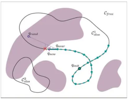
extended to handle the geometric constraints in our problem. Algorithm 4 gives the pseudocode and Figure 4 illustrates the exploration in a simple 2D example. The darker regions in the figure correspond to confor-mations with steric clashes,Ꮿfreebeing the rest of the space. In
general, conformations satisfying closure (in Ꮿclos) are grouped
into different disjoint continuous manifolds.50
We considered two manifoldsᏯclos
1
andᏯclos 2
for this illustration.
The starting point qinit can be a randomly sampled feasible
conformation (e.g., generated by the technique explained above) or
a known conformation (e.g., acquired from the PDB). For execut-ing an expansion step of the RRT, a random conformation qrandis
first sampled inᏯ. qrandneed not satisfy either closure or clash
avoidance constraints. This conformation is only used as a local goal for the exploration. Nevertheless, we have experimentally shown that a guided-random sampling generating qrandclose to the
subset satisfying closure equations improves the process (i.e., a wider portion of the space is explored in less time) in relation to a uniform random sampling.51
For this, the configuration parameters corresponding to the independent variables of the closure equa-tions, qa, are generated by the function S
AMPLE_qa(Algorithm 3),
explained above. Then, the nearest node in the current tree, qnear,
Figure 4. Incremental exploration ofᏯfeasusing an RRT-like technique.
is selected using a distance metric inᏯ. A new conformation qfeas
is iteratively pulled from qneartoward qrand. The pulled
conforma-tion must remain in the feasible subset. The closure constraint is maintained as follows. A conformation qstepis obtained by
inter-polating qnearand qrandfollowing a law (e.g., linear interpolation).
The closure equations are then solved for the passive variables of the backbone conformation (called qp
above). If the solution in the same manifold as qnearexists, then the conformation satisfying
closure, q⬘step, is checked for clashes. The process goes on until one
of the feasibility conditions is violated. The new node of the tree,
qnew, is an intermediate conformation between qnearand the last
obtained qfeas. We use a Gaussian sampling between qfeasand qnear
to obtain it.
Several criteria can be adopted for stopping the exploration. The simplest one is to build the tree until it contains a given number of nodes. The drawback is that this criterion is not related to a coverage of the explored region. We believe that an estimation of this coverage could be deduced from the number nfail of
consecutive times the algorithm fails when trying to expand the tree. A similar relationship has been demonstrated in related meth-ods.16
While the infinite solutions of the global inverse kinematics problem are grouped into different disjoint continuous manifolds and collision-free portions of each manifold can be also disjoint, the explained algorithm can explore only a region inᏯfeas. Several
starting points are required for exploring the different connected
components of Ꮿfeas. An algorithm combining RRT and PRM
techniques could be used for the exploration of the whole subset.
Exploration with Flexible Geometry
Considering fixed values for bond lengths, bond angles, and dou-ble-bond torsion angles is a well-accepted assumption that reduces the complexity of the structural analysis of molecules. However, it implies a severe restriction for conformational space exploration.52
The rigid geometry assumption can be relaxed by allowing a slight variation of these parameters within given intervals. Han-dling these new variables is not a hard problem for our exploration algorithm, proceeding as follows. To generate a conformation
qrand, parameters d, ␣, and (see above) are first randomly
sampled within the defined intervals. Then, the approach explained in the Conformational Sampling section can be used. In the incre-mental variation of the selected conformation qneartoward qrand,
the new parameters are treated like the rest of the (nonpassive) variables (i.e., they are interpolated following a given law).
First Results: Loop 7 Motions of Amylosucrase from Neisseria Polysaccharea
Amylosucrase (AS) is a glucansucrase that catalyzes the synthesis of an amylose-like polymer from sucrose. In the Carbohydrate-Active enZYme database (CAZy) (http://afmb.cnrs-mrs.fr/⬃cazy/ CAZY/index.htm), this enzyme is classified in family 13 of glu-coside-hydrolases (GH), which mainly contains starch-converting enzymes (hydrolases or transglycosidases). Remarkably, this en-zyme is the only polymerase acting on sucrose substrate reported in this family, all the other glucansucrases being gathered in GH
family 70. Which structural features are involved in AS specificity is an important fundamental question. Indeed, the structural sim-ilarity of AS to family 13 enzymes is high. The 3D structure reveals an organization in five domains.53
Three of them are commonly found in family 13: a catalytic (/␣)8barrel domain, a
B domain between-strand 3 and ␣-helix 3 (loop 3), and a C terminal Greek key domain. Two additional domains are found in AS only: a helical N-terminal domain and a domain termed B⬘, formed by an extended loop between-strand 7 and ␣-helix 7. Domain B⬘ partially covers the active site located at the bottom of a pocket and is mainly responsible for this typical architecture. Recently, cocrystallization of AS with maltoheptaose revealed the presence of two maltoheptaose binding sites, the first (OB1) in the main access channel to the active site and a second (OB2) at the surface of domain B⬘. Soaking AS crystals with sucrose also revealed the presence of a second sucrose binding site (SB2) different from the active site initially identified.54The comparison
of the various structures obtained suggests that motion of the 17-residue fragment of domain B⬘ starting at residue Gly433 and ending at residue Gly449, consecutive to oligosaccharide binding, could facilitate sucrose translocation from SB2 to the active site. In the following part, this fragment will be called loop 7. This loop could play a pivotal role responsible for the structural change and the polymerase activity. In this context, molecular simulation of loop 7 motion appears to be crucial to gain new insight into AS structure–function relationships.
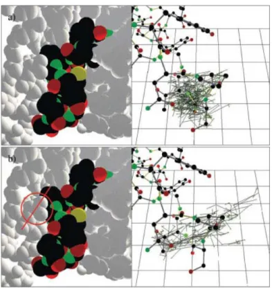
Figure 5 shows the crystallographic structure of AS and the location of the residues we mention in the following paragraphs. The model for our tests was created from the PDB file containing this structure (PDB ID: 1G5A), considering loop 7 as an articu-lated mechanism and the rest of the atoms as static elements. Atoms were modeled with 70% of their vdW radii. Images on the left in Figure 6 represent the articulated vdW model of the loop and a portion of its environment. Under our modeling assumptions, the results of the geometric exploration showed that only slight conformational variations of the loop are possible if the backbone integrity is maintained and steric clashes are avoided. The image on the right in Figure 6(a) shows the skeleton of the articulated segment and a representation of one of the RRTs computed for this test. Nodes of the RRT are graphically represented by the positions explored by the C␣atom of Ser441, the middle residue of the loop. This result contradicts presupposed significant loop fluctuations. Of course, our approach is not deterministic and therefore we cannot guarantee that such a motion does not exist. However, after several exhaustive tests we can assert that the probability of its existence is low. The average size of the constructed RRTs is 1000 nodes, for which about 4000 random conformations and 20,000 complete collision tests were necessary. The average computing time was 1 h.* Note that computing time is mostly spent in collision detection. The generation of random conformations is fast. For this loop, computing a conformation-satisfying closure (including the update of all the frames and atom positions) takes less than 0.1 s with a nonoptimized implementation. The confor-mational sampling used by the exploration algorithm (i.e.,
guided-*Tests were performed using a Sun Blade 100 workstation with a 500-MHz UltraSPARC-IIe processor.
random sampling of qa
without solving the closure equations for
qp
) demands only about 0.01 s per conformation.
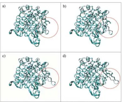
Several structural elements, and mainly loop 3 (residues 183–262), restrain the mobility of loop 7. Residue Asp231 was identified as the main “geometric lock” responsible for the loop 7 enclosing. The side-chain of this residue was removed from the model to simulate a possible conformational change of this chain or even of the whole loop 3. The conformational explo-ration in this case showed that the loop is able to effect the expected motions keeping geometric constraints. The C␣atom of Ser441 can be dislocated more than 9 Å from its crystallo-graphic position. Several tests were performed to see if the random nature of the approach could have an important influ-ence on the nature of the results. Similar motions were obtained for all of them. The loop moves almost as a rigid body with hinges at the extreme residues. Considerable variations of the backbone dihedral angles are concentrated in residues 433– 436 and 446 – 449. Figure 6(b) shows the representation of the RRT constructed in one of these tests. The images in Figure 7 correspond to four frames of the conformational change en-coded in the RRT. Therefore, an “opening/closing” mechanism similar to other enzymes (e.g., refs. 24 and 55), termed
confor-mational gating, is suspected for this loop. The role that residue
Asp231 could play in this mechanism is being investigated. Directed mutagenesis experiments, replacing residue Asp231 by glycine, are currently being developed.
Discussion and Prospects
We proposed geometric techniques aimed at providing powerful filters for conformational sampling and search methods. Our solution to the loop-closing problem is computationally efficient and its per-formance is only slightly affected by the length of the molecular chain. To the best of our knowledge, only the CCD algorithm recently proposed in ref. 8 offers a similar performance. While this optimiza-tion-based algorithm converges to an approximate closure solution starting from a nearly open conformation of the loop, our RLG sampling method computes exact solutions to the closure problem. Also, one disadvantage pointed out in ref. 8 is that the CCD optimi-zation technique, which considers one degree of freedom at a time, may favor large changes in the first residues of the loop. By compar-ison, the random strategy of RLG produces more uniformly distrib-uted samples, better suited for exploration of the conformational space.
Our algorithms are currently implemented within the motion planning platform Move3D56
developed at LAAS for robotics applications. No particular consideration has been given to reduc-ing computation time in the present implementation, which is aimed at demonstrating the efficacy of the proposed techniques. More extensive experimental tests and performance comparisons remain for future work, based on an optimized version taking advantage of the specifics of molecular models. We started the development of such an optimized version and a standalone library that could be made accessible to the scientific community.
Figure 6. Exploration (a) with and (b) without the side-chain of Asp231.
[Color figure can be viewed in the online issue, which is available at www.interscience.wiley.com.]
Concerning the avoidance of steric clashes, collision detection algorithms combined with smart sampling techniques constitute an attractive alternative to methods producing optimization-based re-arrangements. We are developing a tailored collision detection algorithm for molecular models that should perform faster than the generic checker currently used. In addition, a different progressive process for building backbone conformations is going to be tried. In contrast to the described sampling approach, clashes between the backbone atoms and the static environment will be checked after each step of the RLG algorithm.
In our current implementation, values for all variable dihedral angles in the side-chains and backbone are randomly sampled in the interval (⫺, ]. As in other related techniques, our approach could handle information on the statistically preferred values of these angles (e.g., from Ramachandran plots by residue type). Using this information, many local steric clashes should be im-plicitly avoided.
Concerning the exploration technique, we are working on a method for pruning branches of the RRT to decrease the size of this data structure, thus increasing the speed of the search process. Preliminary results using a visibility-based heuristic16seem
prom-ising.
The algorithms presented in this article treat conformations of a molecular segment in a static environment. The extension of these algorithms to handle the flexibility of side-chains in this environment could be done without difficulty. Handling several loops that share the same region of the space (e.g., antibody hypervariable loops57
) is an interesting extension we expect to develop.
The first results of the application of our robotic approach to molecular models show the potential of this technique. A fast geometric analysis can help find the answer to important
biochem-ical questions such as: what are the crucial residues in the bio-chemical reaction? and what are the possible conformational changes?
Although our next goal is to improve this geometrically con-strained exploration, the final aim is to incorporate the energetic analysis into the incremental search technique. An energy function can easily be integrated into this kind of exploration algorithm. Indeed, impressive results have been obtained by conformational search methods inspired by sampling-based motion planning tech-niques applied to computer-assisted drug design,29
protein fold-ing,27,58
and ligand–protein docking.59,60
Given this energy func-tion, geometrically feasible conformations generated by our approach could be evaluated and labeled, and then only the subset of the conformational spaceᏯlow Ebelow a certain energetic limit
should be explored.
Acknowledgments
The collaboration and advice of the following people has been essential for carrying out this work: Gwe´nae¨lle Andre´ (INRA, Nantes), Paul Bates (CRUK, London), Patrick Danes (LAAS-CNRS, Toulouse), David Guieysse (INSA, Toulouse), Marc Renaud (LAAS-CNRS, Toulouse), Lluı´s Ros (IRI-CSIC, Barce-lona), and Vicente Ruiz (IRI-CSIC, Barcelona). This work has been partially supported by the interdisciplinary CNRS project BioMove3D and the European project IST-37185 MOVIE.
References
1. Leach, A. R. Molecular Modeling: Principles and Applications; Long-man: White Plains, NY, 1996; Chapter 8.
Figure 7. Simulated conformational gating of loop 7 in AS. [Color figure can
be viewed in the online issue, which is available at www.interscience. wiley.com.]
2. Frenkel, D.; Smit, B. Understanding Molecular Simulation: From Algorithms to Applications; Academic Press: New York, 1996. 3. Go, N.; Scheraga, H. A. Macromolecules 1970, 3, 178–187. 4. Manocha, D.; Zhu, Y.; Wright, W. CABIOS 1995, 11, 71– 86. 5. Wedemeyer, W. J.; Scheraga, H. A. J Comput Chem 1999, 20, 819 –
844.
6. Shenkin, P. S.; Yarmush, D. L.; Fine, R. M.; Wang, C.; Levinthal, C. Biopolymers 1987, 26, 2053–2085.
7. Zheng, Q.; Rosenfeld, R.; Vajda, S.; DeLisi, C. J Comput Chem 1993, 14, 556 –565.
8. Canutescu, A. A.; Dunbrack, R. L. Jr. Protein Sci 2003, 12, 963–972. 9. Oliva, B.; Bates, P. A.; Querol, E.; Aviles, F. X.; Sternberg, M. J. E.
J Mol Biol 1997, 266, 814 – 830.
10. van Vlijmen, H. W. T.; Karplus, M. J Mol Biol 1997, 267, 975–1001. 11. Bruccoleri, R. E.; Karplus, M. Biopolymers 1987, 26, 137–168. 12. Moult, J.; James, M. N. G. Proteins 1986, 1, 146 –163.
13. Lotan, I.; Schwarzer, F.; Halperin, D.; Latombe, J. C. In Proceedings of the 18th ACM Symposium on Comp Geom; Barcelona, 2002; p 43–52.
14. Latombe, J. C. Robot Motion Planning; Kluwer Academic: Boston, 1991.
15. Kavraki, L. E.; Sˇvestka, P.; Latombe, J. C.; Overmars, M. IEEE Trans Rob Autom 1996, 12, 566 –580.
16. Sime´on, T.; Laumond, J. P.; Nissoux, C. Adv Rob J 2000, 14, 477– 494.
17. LaValle, S. M. In Control Problems in Robotics; Bicchi A.; Chris-tensen H. I.; Prattichizzo D., Eds.; Springer-Verlag: Berlin, 2002; p 19 –37.
18. Corte´s, J.; Sime´on, T.; Laumond, J. P. In Proceedings of the IEEE International Conference on Robotics & Automation; IEEE: Washing-ton D.C., 2002; p 2141–2146.
19. Corte´s, J.; Sime´on, T. In Proceedings of the IEEE International Con-ference on Robotics & Automation; IEEE: Taipei, 2003; p 4354 – 4359.
20. Contreras-Moreira, B.; Fitzjohn, P. W.; Bates, P. A. Appl Bioinfo 2002, 1(4), 177–190.
21. Tramontano, A.; Leplae, R.; Morea, V. Proteins 2001, Suppl. 5, 45, 22–38.
22. Baker, D.; Sˇali, A. Science 2001, 295, 93–96.
23. Fiser, A.; Do, R. K.; Sˇali, A. Protein Sci 2000, 9, 1753–1773. 24. Osborne, M. J.; Schnell, J.; Benkovic, S. J.; Dyson, H. J.; Wright, P. E.
Biochemistry 2001, 40, 9846 –9859.
25. Janin, J.; Henrick, K.; Moult, J.; Eyck, L. T.; Sternberg, M. J. E.; Vajda, S.; Vakser, I.; Wodak, S. J. Proteins 2003, 52, 2–9. 26. Metropolis, N.; Rosenbluth, A. W.; Rosenbluth, M. N.; Teller, A. H.;
Teller, E. J Chem Phys 1953, 21, 1087–1092.
27. Apaydin, M. S.; Brutlag, D. L.; Guestrin, C.; Hsu, D.; Latombe, J. C. In Proceedings of RECOMB; Washington D.C., 2002; p 12–21. 28. Ramachandran, G. N.; Sasisekharan, V. Adv Prot Chem 1968, 23,
283– 438.
29. LaValle, S. M.; Finn, P. W.; Kavraki, L. E.; Latombe, J. C. J Comput Chem 2000, 21, 731–747.
30. Scott, R. A.; Scheraga, H. A. J Chem Phys 1966, 44, 3054 –3069. 31. Craig, J. J. Introduction to Robotics: Mechanics and Control;
Addison-Wesley: Reading, MA, 1989; Chapter 3.
32. Zhang, M.; Kavraki, L. E. J Chem Info Comp Sci 2002, 42, 64 –70.
33. Edelsbrunner, H. In Robotics: The Algorithmic Perspective (WAFR1998); Agarwal P.; Kavraki L. E.; Mason M.; Eds.; A. K. Peters: Boston, 1998; p 265–277.
34. Bondi, A. J Phys Chem 1964, 68, 441– 451.
35. Nielsen, J.; Roth, B. Proc NATO Adv Study Inst Comp Meth Mech 1997, 1, 233–252.
36. Lee, H. Y.; Liang, C. G. Int J Mech Mach Theory 1988, 23, 209 –217. 37. Raghavan, M.; Roth, B. In Proceedings of the Int Symp Rob Res;
Tokyo, 1989; 314 –320.
38. Manocha, D.; Canny, J. IEEE Trans Rob Autom 1994, 10, 648 – 657. 39. Renaud, M. In Proceedings of the Int Conf Mech Design & Prod Cairo,
2000; p 15–25.
40. Crippen, G. M. J Comput Chem 1992, 13, 351–361.
41. Celaya, E.; Torras, C. In Computational Kinematics; Angeles J.; Hommel G.; Kova´cs P., Eds., Kluwer Academic: Dordrecht, 1993; p 85–94.
42. Ricard, R.; Gosselin, C. M. J Mech Design 1998, 120, 269 –278. 43. Merlet, J. P. J Intell Rob Sys 1995, 13, 143–160.
44. Pauling, L. The Nature of the Chemical Bond; Cornell University Press: Ithaca, NY, 1960.
45. Angeles, J. Fundamentals of Robotic Mechanical Systems; Springer-Verlag: New York, 2003.
46. Kwakernaak, H.; Sebek, M. IEEE Trans Autom Control 1994, 39, 315–328.
47. Lin, M.; Manocha, D.; Cohen, J.; Gottschalk, S. In Algorithms for Robotic Motion and Manipulation (WAFR1996); Laumond J.-P.; Overmars M. H., Eds., A. K. Peters: Boston, 1997; p 129 –141. 48. Jime´nez, P.; Thomas, F.; Torras, C. In Robot Motion Planning and
Control; Laumond J.-P., Ed.; Springer-Verlag: Berlin, 1998; p 305– 343.
49. van Geem, C.; Sime´on, T. LAAS Report 01073; Toulouse, 2001. 50. Burdick, J. W. In Proceedings of the IEEE Conference on Robotics
and Automation, Scottsdale, AZ, 1989; p 264 –270.
51. Corte´s, J. PhD Thesis; Institut National Polytechnique de Toulouse, 2003.
52. Bruccoleri, R. E.; Karplus, M. Biopolymers 1985, 18, 2767–2773. 53. Skov, L. K.; Mirza, O.; Henriksen, A.; de Montalk, G. P.;
Remaud-Simeon, M.; Sarc¸abal, P.; Willemot, R. M.; Monsan, P.; Gajhede, M. J Biol Chem 2001, 276, 25273–25278.
54. Skov, L. K.; Mirza, O.; Sprogoe, D.; Dar, I.; Remaud-Simeon, M.; Albenne, C.; Monsan, P.; Gajhede, M. J Biol Chem 2002, 277, 47741– 47747.
55. Derreumaux, P.; Schlick, T. Biophys J 1998, 74, 72– 81.
56. Sime´on, T.; Laumond, J. P.; Lamiraux, F. In Proceedings of the IEEE International Conference on Robotics and Automation; Seoul, 2001; p 25–30.
57. Bruccolerim, R. E.; Haber, E.; Novotny, J. Nature 1988, 335, 564 – 568.
58. Amato, N. M.; Dill, K. A.; Song, G. J Comp Biol 2002, 9, 149 –168. 59. Apaydin, M. S.; Singh, A. P.; Brutlag, D. L.; Latombe, J. C. In Proceedings of the IEEE International Conference on Robotics and Automation; Seoul, 2001; p 932–939.
60. Bayazit, O. B.; Song, G.; Amato, N. M. In Proceedings of the IEEE International Conference on Robotics and Automation; Seoul, 2001; p 954 –959.