Photospheric flows measured with TRACE

HAL Id: hal-02178310

https://hal.archives-ouvertes.fr/hal-02178310

HAL is a multi-disciplinary open access

archive for the deposit and dissemination of sci-entific research documents, whether they are pub-lished or not. The documents may come from teaching and research institutions in France or abroad, or from public or private research centers.

L’archive ouverte pluridisciplinaire HAL, est destinée au dépôt et à la diffusion de documents scientifiques de niveau recherche, publiés ou non, émanant des établissements d’enseignement et de recherche français ou étrangers, des laboratoires publics ou privés.

Photospheric flows measured with TRACE

J. Krijger, T. Roudier, M. Rieutord

To cite this version:

J. Krijger, T. Roudier, M. Rieutord. Photospheric flows measured with TRACE. Astronomy and Astrophysics - A&A, EDP Sciences, 2002, 387 (2), pp.672-677. �10.1051/0004-6361:20020405�. �hal-02178310�

DOI: 10.1051/0004-6361:20020405

c

ESO 2002

_Astrophysics

&

Photospheric flows measured with TRACE

1

Sterrekundig Instituut, Postbus 80 000, 3508 TA Utrecht, The Netherlands e-mail: J.M.Krijger@astro.uu.nl

2

Laboratoire d’Astrophysique de Toulouse, Observatoire Midi-Pyr´en´ees, 14 avenue E. Belin, 31400 Toulouse, France

e-mail: roudier@bagn.obs-mip.fr; rieutord@obs-mip.fr Received 16 January 2002 / Accepted 14 March 2002

Abstract. We analyse white-light image sequences taken with the Transition Region and Coronal Explorer

(TRACE) using an optimised local correlation tracking (LCT) method to measure the horizontal flows in the quiet solar photosphere with high spatial (1 arcsec) and temporal (5 min) resolution. Simultaneously taken near-ultraviolet images from TRACE confirm that our LCT-determined flows recover the actual supergranulation pattern, thus proving that the topology of the horizontal flow distribution and network assembly may be studied from long-duration TRACE white-light sequences with our method.

Key words. Sun: photosphere – Sun: chromosphere – Sun: granulation

1. Introduction

Convective flows dominate the stucture of and the en-ergy transport in the outer parts of the Sun up to the deep photosphere. Understanding the convective flow and its interaction with the magnetic fields is important since convective motions are believed to drive many important processes on the sun, e.g., (i) – the solar dynamo through interaction with solar rotation, (ii) – the p-mode oscil-lations that are used to probe the solar interior, (iii) – magneto-hydrodynamic waves which supply energy to the chromosphere, and (iv) – foot-point motions that lead to magnetic reconnection which may heat the corona.

The most visible product of convection is the solar granulation with a characteristic scale of 1000 km, life-time of about 10 min (e.g., Bray et al. 1984), and easily recorded in broadband images. The solar granulation is re-produced remarkably well in numerical simulations (e.g., Stein & Nordlund 1998). The larger granulation scales, meso- and supergranulation, are less understood. The ex-istence of convection at the mesogranular scale is still in debate (e.g., Rieutord et al. 2000; Ploner et al. 2000), while study of the supergranular pattern is difficult because it does not show directly in white light whereas the mag-netic network and the chromospheric brightness network map supergranular cell boundaries only incompletely. The new technique of time-distance helioseismology (Duvall et al. 1993) has become very popular for studying the

Send offprint requests to: J. M. Krijger,

e-mail: J.M.Krijger@astro.uu.nl

supergranulation, but results in controversal findings (e.g., Hathaway et al. 2002) which require further investiga-tion. The supergranule scales are still debated (see Beck & Duvall 2001), with the current estimates for the length scale between 13 Mm and 35 Mm (e.g., Hagenaar et al. 1997) and a lifetime between 15 hours and 52 hours de-pending on scale (e.g., Wang & Zirin 1989; Simon et al. 1995).

As shown by Rieutord et al. (2001) the flow speeds de-termined from brightness changes describing granular mo-tions are an indication of the horizontal motion of the as-sociated matter. Tracking this granular structure enables determination of the longer-lived and wider horizontal flows (November & Simon 1988) and one may so study the assembly and topological evolution of the magnetic network at these scales.

Different attempts (e.g., Leighton et al. 1962; Brandt et al. 1994; 1999, 2000) have been made to determine quiet-sun surface flows from ground-based observations. These observations were limited by small field of view (FOV), short duration, and the presence of seeing which hampers precise flow evaluation. Seeing is best avoided by putting telescopes in orbit. The SOUP instrument on-board Spacelab 2 collected a sequence of too short a du-ration (28 min) to study supergranular (>15 hrs) pat-tern changes (Simon et al. 1988). The MDI instrument on-board the SOHO satellite can observe for much longer duration but is limited by the fixed pointing of its high resolution field. The line-of-sight velocity images obtained

Article published by EDP Sciences and available at http://www.aanda.org or http://dx.doi.org/10.1051/0004-6361:20020405

J. M. Krijger et al.: Photospheric flows measured with TRACE 673

by MDI are much used with time-distance helioseismology (e.g., De Rosa et al. 2000; 2002).

Image sequences from the TRACE satellite (Handy et al. 1999) do not suffer from seeing and have a some-what better resolution (1 arcsec) than MDI (1.3 arcsec). TRACE offers a large FOV (512× 512 arcsec2) and long duration observations (up to a week) by following a given area on the solar surface by correcting for solar rotation. Also, TRACE permits quasi-simultaneous observations in both white light (low photosphere) and near-ultraviolet (upper photosphere) wavelengths. The bright chromo-spheric network visible in the near-ultraviolet wavelengths can be used to show the location of the magnetic network, which is governed by the flows, in the absence of magne-tograms allowing a direct check. However, so far it was not clear whether the TRACE resolution of 1 arcsec is good enough to obtain reliable flow estimates since it resolves the granulation which is to be used as flow tracer only partially.

In this paper we test whether it is possible to use the TRACE white light observations despite their low resolu-tion for measuring horizontal velocity fields, by optimising the LCT method of November & Simon (1988) and using “isotropic divergence” (Roudier et al. 1999; Rieutord et al. 2000). The (dis)advantages of the LCT and other tracking techniques used by different authors are presented and dis-cussed in Roudier et al. (1999). For a discussion of previous studies using feature tracking, see Rieutord et al. (2000). Our test proves that our modified LCT method with opti-mised parameters and data reduction can be used to derive horizontal flows from longer TRACE white-light image sequences.

The organisation of the paper is as follows. The obser-vations and reductions are presented in the next section. In Sect. 3 we display the results of the analysis with the conclusions following in Sect. 4.

2. Observations and reduction 2.1. TRACE sequence

We use a TRACE image sequence taken on October 14, 1998 between 8:12–12:00 UT. TRACE observed a very quiet rectangular area of the solar surface at disk center (see Fig. 1) in three ultraviolet passbands (centered at λ = 1700 ˚A, 1600 ˚A, and 1550 ˚A) and a broadband white-light passband. A nominal cadence of 21 s for each individual passband (but longer occasionally) was used. Only 512× 512 pixel2of the 1024× 1024 pixel2TRACE CCD camera with 0.5 arcsec pixels (366 km on the Sun) were read out due to telemetry limitations. The satellite pointed at a fixed location on the apparent solar disk without following solar rotation during the observation. The observations are specified in Table 1. Figure 2 shows as example pair of white-light and 1700 ˚A images.

In this analysis only the lower half of the observed field (256× 128 arcsec2) was used, due to computer resource restrictions. The images were reduced following standard

N

Fig. 1. Solar location of the field observed with TRACE on

October 14, 1998, slightly off disk center. Only the lower half of this field was used for the analysis presented in this paper. The grid shows heliocentric longitude and latitude.

procedures1 (dark current subtraction, flat field correc-tion). The sequences were subsequently aligned to remove solar rotation and satellite jitter using cross-correlation aligning the ultraviolet images to other images of the same passband and to the other passbands within a few tenths of a pixel. Differential rotation across the field during the entire sequence had only a small effect (0.4 pixel) and was neglected. Due to solar rotation and satellite jitter only part of the FOV was fully sampled (452× 246 pixel2_,

226×123 arcsec2_{or 165×90 Mm}2_{). More details on these}

data and its reduction are given in Krijger et al. (2001). More information on reducing TRACE data is available in the TRACE Analysis Guide2_.

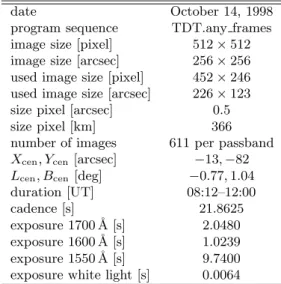
Table 1. TRACE observations used in this paper.

date October 14, 1998

program sequence TDT.any frames image size [pixel] 512× 512 image size [arcsec] 256× 256 used image size [pixel] 452× 246 used image size [arcsec] 226× 123 size pixel [arcsec] 0.5

size pixel [km] 366

number of images 611 per passband

Xcen, Ycen[arcsec] −13, −82

Lcen, Bcen [deg] −0.77, 1.04

duration [UT] 08:12–12:00

cadence [s] 21.8625

exposure 1700 ˚A [s] 2.0480 exposure 1600 ˚A [s] 1.0239 exposure 1550 ˚A [s] 9.7400 exposure white light [s] 0.0064

2.2. Local correlation tracking

In order to take out the five-minute oscillation, all horizon-tal movements faster then 4 km s−1were removed from the

1

http://www.lmsal.com/solarsoft/

2

Fig. 2. Top: sample white-light image taken by TRACE at

10:03 UT, Oct. 14 1998. With a resolution of only 1 arcsec TRACE only resolves the larger granules. Smaller granules can jointly appear erroneously as large granules when close enough. No large-scale or magnetic structures are discernable. Bottom: corresponding 1700 ˚A image taken by TRACE 2 s earlier. The brightest features belong to the chromospheric network. The latter stands out more clearly in the time-average display at bottom-left in Fig. 6. Axes: X and Y in arcsec from disk center.

white-light sequence by 3D Fourier filtering (Title et al. 1989).

Subsequently, each individual white-light image was enlarged by a factor of 4 (using interpolation) in order to increase the number of points used in subsequent correla-tion computacorrela-tions since the noise in the velocity measure-ments is proportional to 1/√N where N is the number

of points used for the correlation. A test on blurred high resolution ground-based observations showed that this en-largement allows better recovery of the actual velocity fields.

The method used below is described in more detail in Roudier et al. (1999). After enlargement the images were filtered using a 1 arcsec2 _{Gaussian window. Tests}

showed that a larger window samples multiple granules and measures only their group-averaged motion, while a smaller window measures details below the resolution of TRACE (1 arcsec) and generates meaningless results. Subsequently, the images were transformed into a binary map of granules, using local curvature of the intensity pat-tern to identify granules following Strous (1995).

Horizontal velocity fields were calculated using these binarised maps with the LCT method of November & Simon (1988) with 5 min resolution. Using LCT on binarised data was named the LCTbin method by

Roudier et al. (1999). For each 5 min temporal window

Fig. 3. Horizontal flows in a partial cutout from the measured

horizontal velocity field at 1 arcsec resolution between 10:10– 10:15 October 14 1998. Each arrow shows the direction and magnitude of the velocity at a particular point with 1 arcsec length corresponding to 0.25 km s−1. Axes: X and Y in arcsec from disk center.

Fig. 4. Histogram of all measured mean horizontal velocities

(both in x and y direction), with 3σ estimates (shaded con-tours). Most velocities are below 1 km s−1, with a maximum around 0.25 km s−1.

15 sequential images were used. A test showed that us-ing an artificial cadence of∼1 min (3 images per tempo-ral window) instead of 21 sec yields similar results. The period of 5 min was used as a compromise between the (mean) lifetime of the granules and noise in the resulting flow maps.

Figure 3 shows a sample result. Large-scale (∼7 Mm) diverging and converging areas are visible as a mesoscale pattern. The statistical distribution of the measured flow speeds is shown in Fig. 4. The lower cut-off is due to the angular resolution set by the TRACE CCD pixel size. Most mean velocities are below 1 km s−1. This distribu-tion is shifted towards the lower velocities compared to the granular mean velocity found in Roudier et al. (1999), due to the tendency of the LCTbinmethod of smoothing

out the smaller and faster patches in the velocity fields. After the computation of successive mean-flow maps covering the whole sequence duration, one can insert arti-ficial tracers or “corks” that follow horizontal motions over a longer lifetime than that of individual granules, and so mapping longer-lived flows (Simon et al. 1988). Figure 5 shows the final position of such corks, inserted at the start

J. M. Krijger et al.: Photospheric flows measured with TRACE 675

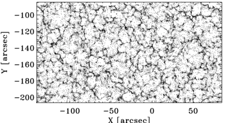
Fig. 5. This plot shows the final positions of about 30 000 “corks” or tracers after 4 hours, that were initially dis-tributed regularly and allow to freely flow on the velocity fields. Some tracers have not yet reached their final destination, but large scale structures are visible. Axes: X and Y in arcsec from disk center.

of the flow-map sequence. Large (∼22 Mm) cell-like closed structures are visible, filled with smaller (∼7 Mm) cells that are less well outlined. The large cells correspond to the supergranular network as we demonstrate in Figs. 6 and 7. The smaller structures result at least partially from the short sequence duration by showing corks that have not yet reached their final supergranular-cell boundary destination.

2.3. Isotropic divergence

A quantity that can be derived from flow patterns is the horizontal divergence∇ · vxywhich furnishes another

pre-sentation of the surface flows. Our interest is into sources of divergence/convergence, those locations where matter presumably appears at the surface by flowing upward (di-vergence) and where matter presumably disappears from the surface by flowing downwards (convergence), respec-tively. However, using the classical divergence calculation, one also finds a high divergence or convergence value at a particular location when the surrounding area as a whole is horizontally accelerating or decelerating. We therefore employ the “isotropic divergence” instead (Rieutord et al. 2000). We briefly describe both methods here.

Calculating the divergence at a certain point in a reg-ular grid is a straightforward procedure by summing the difference in velocity (in orthogonal directions) of the 4 adjacent points. The mathematical definition for the classic divergence at location (x, y) in a regular dis-crete grid is:

vx(x+1, y)− vx(x−1, y) + vy(x, y +1)− vy(x, y−1)

2W , (1)

with W the distance between two gridpoints and vx, vythe

respective velocity components. The averaged horizontal divergence over the entire duration of the observation is shown in the top-left panel of Fig. 6.

The isotropic divergence is defined in each point as the sum of the difference (normalised by the distance) of the

projected vector components of the velocity on the axis of the symmetrical points relative to the central one, in all the directions and computed for the two gridpoint-rings around this central point (8 points for the first ring and 16 points for the second ring). The mathematical defini-tion for the isotropic divergence in locadefini-tion (x, y) is:

2 X sx=−2 2 X sy=−2 sxvx(x+sx, y +sy) + syvy(x+sx, y +sy) 2W (s2 x+ s2y) , (2)

with sx, sy the gridpoint distance from x, y in their

re-spective directions, which are not allowed to be zero at the same time (i.e., the velocity in the central point is not used for the divergence calculations). The resulting amplitudes peak at isotropic divergence/convergence sites such as exploding granules and sink holes. The averaged horizontal isotropic divergence is shown in the middle-left panel of Fig. 6.

3. Results 3.1. Divergence

Both the classic and isotropic divergences were evaluated and subsequently averaged over the total duration of the observation (8:12–12:00 UT). The results are shown in the two upper panels in the lefthand column of Fig. 6. Using isotropic divergence yields a coarser pattern with a clearer indication of cellular structure at supergranular scale which is outlined by darker-than-average boundary segments.

3.2. Chromospheric network

The capacity of TRACE to simultaneously observe in the ultraviolet and the white-light allows us to compare the cork collection sites in Fig. 5 and the coarse grid-pattern of convergence sites in Fig. 6 to the actual structure of the chromospheric network. The pertinent ultraviolet observa-tions from TRACE are described in more detail in Krijger et al. (2001). The TRACE 1600 ˚A and 1700 ˚A passbands show very similar features as Ca II K2V movies from

ground-based telescopes (Rutten et al. 1999). The bottom-left panel of Fig. 6 shows the temporal average of the entire 1700 ˚A sequence. The chromospheric network stands out much clearer in this time-average display than in the snap-shot image in the lower panel of Fig. 2 because the inter-mittent internetwork features (mostly due to the chromo-spheric three-minute oscillation) average away while the more persistent network features are enhanced.

3.3. Spatial comparison

Comparison of Fig. 6 with Fig. 5 shows that the regions with highest cork density (Fig. 5) correspond closely to the bright ultraviolet network (bottom-left panel of Fig. 6). Similarly, comparing the temporally averaged divergences with the 1700 ˚A temporal average image (lefthand pan-els of Fig. 6) indicates spatial correspondence between

Fig. 6. Top left: classic divergence defined by Eq. (1) averaged over the entire duration (228 min) of the observation. Bright

areas indicate locations where the flows are diverging, dark areas indicate converging flows. Middle left: same as first panel, but showing isotropic divergence as defined by Eq. (2). Large scale structures become more distinct. Bottom left: the average of the 1700 ˚A sequence taken at the same time and location. The greyscale is logarithmic in order to bridge the large contrast. Top right: again showing the time-averaged isotropic divergence but now overlaid with the contours of the bright network from the bottom-left panel. A clear correlation between the dark converging areas and the bright network can be seen. Middle and bottom right: split of the top-right panel into internetwork-only and network-only displays, using a mask defined by the network contours. The split produces yet clearer visualisation of the spatial correlation between the dark converging areas and the bright network. Axes: X and Y in arcsec from disk center, all panels show the same subfield.

the (dark) converging areas and the bright chromospheric network. The righthand panels of Fig. 6 visualises this correlation by showing different comparisons between the isotropic divergence and the 1700 ˚A image. In the top-right panel the isotropic divergence is shown overplotted with the network contours of the 1700 ˚A image. The two lower panels in the righthand column show the difference directly.

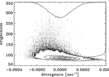
Finally, the spatial correlation between convergence sites and chromospheric network is illustrated in Fig. 7 by plotting 1700 ˚A brightness versus the average diver-gence as a scatter diagram. It shows that most bright net-work features are located at convergence (negative diver-gence) locations. This proves that the surface flows which we have measured with our correlation tracking indeed

represent long-term supergranular motions, even though Fig. 5 shows that not all corks have reached their final position in the supergranular cell borders.

4. Conclusions

We have demonstrated that, although TRACE resolu-tion (1 arcsec) is not good enough to fully resolve the solar granulation, it does suffice to determine the flow patterns over the solar surface that produce and con-trol the topology of the solar network. Using the LCTbin

method high spatial (1 arcsec) and temporal (5 min) res-olutions can be obtained. These resres-olutions have not been achieved before on seeing-free data with such a large FOV (226× 123 arcsec2) and long duration (228 min). TRACE

J. M. Krijger et al.: Photospheric flows measured with TRACE 677

Fig. 7. Correlation between average 1700 ˚A brightness and av-erage velocity field divergence shown as a pixel-by-pixel scatter plot, with density contours replacing individual points where they become too close. The curves along the axes measure the first moments per row and column, respectively. The locations with the brightest network (upward tail of the scatter cloud) correspond to negative divergence in the flow field.

allows a FOV up to 512× 512 arcsec2 _{and observations}

centered at a given (co-rotating) solar location up to a week duration. Combination of such measurements with our method allows study of the distribution and network assembly over long time scales with longer TRACE WL sequences. These higher temporal and spatial resolutions allow a gain in the analysis of the signal (velocity) from high to low frequencies in the two domains. In particular, it helps to distinguish the smoothing effects of the data re-duction and analysis from the solar flow fields at medium and low frequencies (spatial and temporal) and to learn about the influence of the smaller scales on to the largest ones. Our approach allows us to locate more precisely the largest diverging amplitude events of the flow field and to correlate their evolution to the UV bright points (oscilla-tions, mo(oscilla-tions, etc.) which are located on the border of the supergranule.

Acknowledgements. J. M. Krijger’s research is funded by

The Netherlands Organization for Scientific Research (NWO). J. M. Krijger thanks the Observatoire Midi-Pyr´en´ees for their hospitality and financial support during his visit there. We are indebted to R. J. Rutten for suggesting this research and many improvements to the manuscript and to referee J. G. Beck for his valuable comments.

References

Beck, J. G., & Duvall, T. L. 2001, in Helio- and asteroseismol-ogy at the dawn of the millennium, ed. A. Wilson, Procs. of the SOHO 10/GONG 2000 Workshop (ESA SP-464), 577 Brandt, P. N., Rutten, R. J., Shine, R. A., & Trujillo Bueno, J.

1994, in Solar Surface Magnetism, ed. R. J. Rutten, & C. J. Schrijver, NATO ASI Series C 433 (Dordrecht: Kluwer), 251

Bray, R. J., Loughhead, R. E., & Durrant, C. J. 1984, The solar granulation (2nd edition) (Cambridge University Press), 270

De Rosa, M., Duvall, T. L., & Toomre, J. 2000, Sol. Phys., 192, 351

Duvall, T. L., Jefferies, S. M., Harvey, J. W., & Pomerantz, M. A. 1993, Nature, 362, 430

Hagenaar, H. J., Schrijver, C. J., & Title, A. M. 1997, ApJ, 481, 988

Handy, B. N., Acton, L. W., Kankelborg, C. C., et al. 1999, Sol. Phys., 187, 229

Hathaway, D. H., Beck, J. G., Han, S., & Raymond, J. 2002, Sol. Phys., 205, 25

Krijger, J. M., Rutten, R. J., Lites, B. W., et al. 2001, A&A, 379, 1052

Leighton, R. B., Noyes, R. W., & Simon, G. W. 1962, ApJ, 135, 474

November, L. J., & Simon, G. W. 1988, ApJ, 333, 427 Ploner, S. R. O., Solanki, S. K., & Gadun, A. S. 2000, A&A,

356, 1050

Rieutord, M., Roudier, T., Ludwig, H.-G., Nordlund, ˚A., & Stein, R. 2001, A&A, 377, L14

Rieutord, M., Roudier, T., Malherbe, J. M., & Rincon, F. 2000, A&A, 357, 1063

Roudier, T., Rieutord, M., Malherbe, J. M., & Vigneau, J. 1999, A&A, 349, 301

Rutten, R. J., de Pontieu, B., & Lites, B. W. 1999, in High Resolution Solar Physics: Theory, Observations, and Techniques, ed. T. R. Rimmele, K. S. Balasubramaniam, & R. R. Radick, Procs. 19th NSO/Sacramento Peak Summer Workshop, ASP Conf. Ser., 183, 383

Simon, G. W., Title, A. M., Topka, K. P., et al. 1988, ApJ, 327, 964

Simon, G. W., Title, A. M., & Weiss, N. O. 1995, ApJ, 442, 886

Stein, R. F., & Nordlund, A. 1998, ApJ, 499, 914

Strous, L. H. 1995, in Helioseismology, ed. J. Hoeksema, V. Domingo, B. Fleck, & B. Battrick, Proc. of 4th Soho Workshop, ESA SP-376, 213

Title, A. M., Tarbell, T. D., Topka, K. P., et al. 1989, ApJ, 336, 475