From Rules to Constraint Programs with the Rules2CP Modelling Language

HAL Id: inria-00270326

https://hal.inria.fr/inria-00270326v2

Submitted on 11 Apr 2008

HAL is a multi-disciplinary open access

archive for the deposit and dissemination of

sci-entific research documents, whether they are

pub-lished or not. The documents may come from

teaching and research institutions in France or

abroad, or from public or private research centers.

L’archive ouverte pluridisciplinaire HAL, est

destinée au dépôt et à la diffusion de documents

scientifiques de niveau recherche, publiés ou non,

émanant des établissements d’enseignement et de

recherche français ou étrangers, des laboratoires

publics ou privés.

Modelling Language

Francois Fages, Julien Martin

To cite this version:

Francois Fages, Julien Martin. From Rules to Constraint Programs with the Rules2CP Modelling

Language. [Research Report] RR-6495, INRIA. 2008. �inria-00270326v2�

a p p o r t

d e r e c h e r c h e

From Rules to Constraint Programs with the

Rules2CP Modelling Language

François Fages — Julien Martin

N° 6495

Centre de recherche INRIA Paris – Rocquencourt

Fran¸cois Fages , Julien Martin

Th`eme SYM — Syst`emes symboliques ´

Equipes-Projets Contraintes

Rapport de recherche n° 6495 — April 2008 — 30 pages

Abstract: In this paper, we show that the business rules knowledge repre-sentation paradigm, which is widely used in the industry, can be developped as a front-end modelling language for constraint programming. We present a gen-eral purpose rule-based modelling language, called Rules2CP, and describe its compilation to constraint programs over finite domains with reified and global constraints, using term rewriting and partial evaluation. We prove the conflu-ence of these transformations and provide a complexity bound on the size of the generated programs. The expressiveness of Rules2CP is illustrated with a complete library for packing problems, called PKML, which, in addition to pure bin packing and bin design problems, can deal with common sense rules about weights, stability, as well as specific packing business rules which compile efficiently into constraints.

Key-words: Modelling Languages, Constraint Programming, Rules-based Programming, Combinatorial Optimization

R´esum´e : Dans cet article, nous montrons que le paradigme de repr´esentation des connaissances par des r`egles m´etiers, qui est largement utilis´e dans l’industrie, peut ˆetre d´evelopp´e en un langage de mod´elisation pour la programmation par contraintes. Nous pr´esentons un langage de mod´elisation par r`egles `a usage g´en´eral, appel´e Rules2CP, et d´ecrivons sa compilation en des programmes avec contraintes sur les domaines finis avec r´eification et contraintes globales, proc´edant par r´e´ecriture de termes et ´evaluation partielle. Nous prouvons la confluence de ces transformations et donnons une borne de complexit´e sur la taille des programmes g´en´er´es. L’expressivit´e de Rules2CP est illustr´ee par une biblioth`eque compl`ete pour les probl`emes d’empaquetage, appel´ee PKML, qui, en plus des probl`emes purs de remplissage et de conception de containers, peut traiter des r`egles de sens commun sur les poids, la stabilit´e, de mˆeme que des r`egles m´etiers d’empaquetage qui se compilent efficacement en contraintes. Mots-cl´es : Langages de mod´elisation, programmation par contraintes, pro-grammation par r`egles, optimisation combinatoire

1

Introduction

From a programming language standpoint, one striking feature of constraint programming is its declarativity for stating combinatorial problems, describing only the “what” and not the “how”, and yet its efficiency for solving large size problem instances in many practical cases. From a non-expert user standpoint however, constraint programming is not as declarative as one would wish, and constraint programming systems are in fact very difficult to use by non-expert users outside the range of already treated examples. This well recognized dif-ficulty has been presented as a main challenge for the constraint programming community, and has motivated the search for more declarative front-end problem modelling languages, such as most notably OPL [1] and Zinc [2, 3]. In these lan-guages, a problem is modelled with variables, arrays, primitive constraints, set constructs, iterators and quantifiers. Such problem models can then be mapped to constraint programs, mixed integer linear programs [4], combinations of both [1], or local search programs [5] for solving them.

In the industry however, the business rules approach to knowledge represen-tation has a wide audience because of the property of independence of the rules which can be introduced, checked, and modified independently of the others, and independently of any particular procedural interpretation by a rule engine [6]. This provides an attractive knowledge representation scheme for fastly evolv-ing regulations and constraints, and for maintainevolv-ing systems with up to date information.

In this article, we show that the business rules knowledge representation paradigm can be developped as a front-end modelling language for constraint programming. We present a general purpose rule-based modelling language for constraint programming, called Rules2CP. Rules2CP rules are not general condition-action rules, also called production rules in the expert system com-munity, but restricted logical rules, with one head and no imperative actions, and where bounded quantifiers are used to represent complex conditions. They comply to the business rules manifesto [6], and in particular to the indepen-dence from a procedural interpretation by a rule engine. This is concretely demonstrated in Rules2CP by their compilation to constraint programs using a completely different representation. As a consequence, the rule language pro-posed in this paper comes with a simple semantics in classical first-order logic, instead of the default logics usually considered in the rule-based knowledge rep-resentation community [7, 8].

Furthermore, our aim at designing a knowledge modelling language for non-programmers led us to abandon recursion and data strutures such as arrays and lists, and retain only records (feature terms) and finite collections (enumer-ated lists) with quantifiers and aggregates as iterators. In the next section, we present the syntax of Rules2CP with its main predefined functions and pred-icates. We show how search strategies and heuristics can be specified in a declarative manner, and illustrate the main language constructs with simple examples of combinatorial and scheduling problems.

Then in Sec. 2, we formally describe the compilation of Rules2CP models into constraint programs over finite domains with reified constraints, using a term rewriting system and partial evaluation. We prove the confluence of these transformations which shows that the generated constraint program does not depend on the order of application of the rewritings. Furthermore, we provide a

complexity bound on the size of the generated constraint program which reflects the simplicity of the Rules2CP design choices.

Then in Sec. 4, we illustrate the expressive power and efficiency of this approach with a particular Rules2CP library, called the Packing Knowledge Modelling Library (PKML), developed in the EU project Net-WMS1 for deal-ing with real-size non-pure bin packdeal-ing problems comdeal-ing from the automotive industry. In addition to pure bin packing and bin design problems, we show the capability of PKML to express heuristic knowledge and common sense rules about weights, equilibrium and stability constraints [9], as well as business rules taking into consideration industrial requirements and expertise. Furthermore, we show how a large subset of PKML rules can be directly compiled into the geometric global constraint geost [10] and its integrated rule language [11].

Finally in Sec. 5 we discuss the main features of Rules2CP by comparing them to other formalisms: business rules, OPL and Zinc modelling languages, constraint logic programming and term rewriting systems.

We conclude on the generality of this rule-based knowledge modelling lan-guage as a front-end for constraint programming.

2

The Rules2CP Language

2.1

Syntax

Rules2CP is a term rewriting rule language based on first-order logic with bounded quantification and aggregate operators. Its only data structures are integers, strings, enumerated lists and records. Because of the importance of naming objects in Rules2CP, the language includes a simple module system that prefixes names with module and package names, similarly to [12].

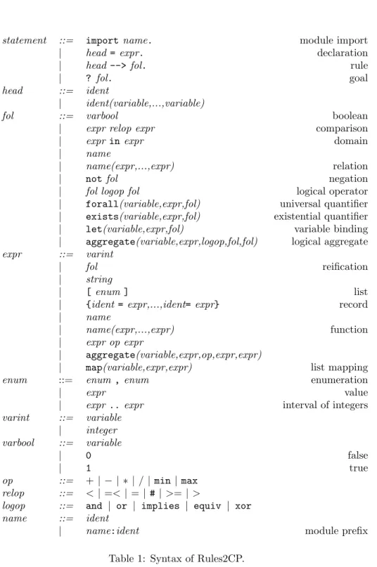
The syntax of Rules2CP is given in Table 2.1. An ident is a word beginning with a lower case letter or any word between quotes. A name is an identifier that can be prefixed by other identifiers for module and package names. A variable is a word beginning with either an upper case letter or the underscore character . The set, denoted by V (E), of free variables in an expression E is the set of variables occurring in E and not bound by a forall, exists, let, map or aggregate operator. The size of an expression or formula is the number of nodes in its tree representation.

In a Rules2CP file, the order of the statements is not relevant. Recursive definitions and multiple definitions of a same head symbol are forbidden. In a rule, L-->R, we assume V (R) ⊆ V (L), whereas in a declaration, H=E, the introduced variables, in V (E) \ V (H), represent the unknown variables of the problem.

An expression expr can be a fol formula considered as a 0/1 integer. This usual coercion between booleans and integers, called reification, provides a great expressiveness [13]. The grammar does distinguish however the logical formulas from other expressions. For instance, a goal cannot be any expression but a logical formula.

The aggregate operator cannot be defined in first-order logic and is a Rule2CP builtin. This operator iterates the application of a binary operator (given in the third argument), to copies of the expression given in the last argument, where

statement ::= import name. module import

| head = expr. declaration

| head --> fol. rule

| ? fol. goal

head ::= ident

| ident(variable,...,variable)

fol ::= varbool boolean

| expr relop expr comparison

| expr in expr domain

| name

| name(expr,...,expr) relation

| not fol negation

| fol logop fol logical operator

| forall(variable,expr,fol) universal quantifier

| exists(variable,expr,fol) existential quantifier

| let(variable,expr,fol) variable binding

| aggregate(variable,expr,logop,fol,fol) logical aggregate

expr ::= varint

| fol reification

| string

| [ enum ] list

| {ident = expr,...,ident= expr} record

| name

| name(expr,...,expr) function

| expr op expr

| aggregate(variable,expr,op,expr,expr)

| map(variable,expr,expr) list mapping

enum ::= enum , enum enumeration

| expr value

| expr .. expr interval of integers

varint ::= variable | integer varbool ::= variable | 0 false | 1 true op ::= + | − | ∗ | / | min | max relop ::= < | =< | = | # | >= | >

logop ::= and | or | implies | equiv | xor

name ::= ident

| name:ident module prefix

the variable in the first argument is replaced by the successive elements of the list given in the second argument. For instance, the product of the elements in a list is defined by product(L)=aggregate(X,L,*,1,X), the maximum by maximum(L)=aggregate(X,L,max,0,X), etc.

Lists of expressions can be formed by enumerating their elements, or intervals of values in the case of integers. For instance [1,3..6,8] represents the list [1,3,4,5,6,8]. Such lists are used to represent the domains of variables in (var in list) formula, and in the answers returned to Rules2CP goals.

The following expressions are predefined for accessing the components of lists and records:

ˆ length(list) returns the length of the list (after expansion of the intervals), or an error if the argument is not a list.

ˆ nth(integer,list) returns the element of the list in the position (counting from 1) indicated by the first argument, or an error if the second argument is not a list containing the first argument.

ˆ pos(element,list) returns the first position of an element occurring in a list as an integer (counting from 1), or returns an error if the element does not belong to the list.

ˆ attribute(record) returns the expression associated to an attribute name of a record, or returns an error if the argument is not a record or does not have this attribute.

Furthermore, records have a default integer attribute uid which provides a unique identifier for each record. The predefined function

ˆ variables(expr)

returns the list of variables contained in an expression. The predefined predi-cates

ˆ X in list

ˆ domain(expr,min,max)

constrains the variable X (resp. the list of variables occurring in the expression expr) to take integer values in a list of integer values (resp. between min and max).

2.2

Predicates for Search

Describing the search strategy in a modelling language is a challenging task as search is usually considered as inherently procedural, and thus contradictory to declarative modelling. This is however not our point of view in Rules2CP. Our approach to this question is to specify the decision variables and the branching formulas of the problem in a declarative manner, as well as the heuristics as preference orderings on variables and values.

Decision variables can be declared with the predefined predicate ˆ labeling(expr)

for enumerating the possible values of all the variables contained in an expres-sion, that is occurring as attributes of a record, or recursively in a record refer-enced by attributes, in a list, or in a first-order formula. This labeling predicate thus provides an easy way to refer to the variables contained in an object or in a formula, without having to collect them explicitly in a list as is usually done in constraint programs. Moreover, Branching formulas can be declared in Rules2CP with the predicate

ˆ search(fol)

This more original predicate specifies a search by branching on all the disjunc-tions and existential quantificadisjunc-tions occurring in a first-order formula. Note that a similar approach to specifying search has been proposed for SAT in [14]. Here however, the only normalization is the elimination of negations in the formula by descending them to the constraints. The structure of the formula is kept as an and-or search tree where the disjunctions constitute the choice points2_.

In Rules2CP, the following optimization predicates specify optimization cri-teria independently of search:

ˆ minimize(expr) for minimizing an expression ˆ maximize(expr) for maximizing an expression

with no restriction on their number of occurrences in a formula. This makes it possible to express multicriteria optimization problems and the search for Pareto optimal solutions according to the lexicographic ordering of the criteria as read from left to right.

2.3

Predicates for Heuristics

Adding the capability to express heuristic knowledge in Rules2CP is mandatory for efficiency. This is done with two predicates for specifying both static and dynamic variable choice as well as value choice heuristics. Dynamic criteria are standard in constraint programming systems, see for instance [15, 16]. The definition of the static criteria use the expressive power of Rules2CP.

The variable choice heuristics predicate takes a list of criteria for or-dering the variables in search. The variables are sorted according to the first criterion when it applies, then the second, etc. The variables for which no crite-rion applies are considered at the end for labeling in an unspecified order. Each criterion has one of the following forms:

ˆ greatest(expr), greatest(expr, option), ˆ smallest(expr), smallest(expr, option), ˆ any(expr), any(expr, option),

ˆ is(expr), is(expr, option),

2_{In order to avoid an exponential growth of the formulas, equiv and xor formulas are kept} as constraints and are not treated as choice points.

where expr is an expression containing the symbol ^ which denotes, for a given variable, the left-hand side of the Rules2CP declaration that introduced a given variable. If the expression cannot be evaluated on a variable, the criterion is ignored. A greatest (resp. smallest) form selects a variable with greatest (resp. smallest) value for the expression. An any form selects a variable for which the expression applies independently of its value. An is form selects a variable if it is equal to the result of the expression. option is a dynamic choice criterion using the following keywords: leftmost, smallest lower bound min, greatest upper bound max, smallest domain ff, or most constrained ffc. The dynamic choice criteria are used in Rules2CP for ordering at run-time the variables which have the same static criteria. For instance, in a bin packing problem, the predicate

variable_choice_heuristics([greatest(volume(^)), smallest(uid(^), ff)])

specifies a lexicographic static ordering of the variables by decreasing volume of the object in which they have been declared, by increasing uid attribute of the object, and for those variables appearing in the same object (i.e. with the same uid), a dynamic ordering by increasing domain size (ff). The static criteria are used at compile-time to order the variables for labelings, while the dynamic criteria are used at run-time by the solver.

The variable choice heuristics predicate takes a list of criteria of the following forms: ˆ up, up(expr), ˆ down, down(expr), ˆ step, step(expr), ˆ enum, enum(expr), ˆ bisect, bisect(expr),

where expr is an expression containing the symbol ^ which denotes the left-hand side of the Rules 2CP declaration that introduces a given variable. A criterion applies to a variable if it matches the expression (a criterion without expression always applies). The different criteria enumerate the values in, respectively, as-cending order (the default), desas-cending order, with binary choices (the default), with a multiple choice, or by dichotomy. For instance, in a bin packing problem, the predicate

value_choice_heuristics([up(z(^)), bisect(x(^)), bisect(y(^))])

specifies the enumeration in ascending order for the z coordinates, and by di-chotomy for the x and y coordinates (and with the default strategy for the other variables).

The capabilities of dissociating the specifications of the variable and value heuristics, and of using static criteria about the objects in which the variables appear, are very powerful. It is worth noticing that this expressive power for the heuristics creates difficulties however for their compilation into constraint systems that mix both kinds of strategies in a single option list, and for which one cannot expresses different value choice heuristics for different variables [16]. For convenience in Rules2CP, the dynamic heuristic criteria can also be added to the labeling predicate as an optional argument.

2.4

Simple Examples

Example 1 The N-queens problem can be modelled in Rules2CP with declara-tions for creating a list of records representing the position of each queen on the chess board, and with one rule for stating when a list of queens do not attack each other, another rule for stating the constraints of a problem of size N , and a goal for stating the size of the problem to solve:

q(I) = {row=_, column=I}. board(N) = map(I, [1..N], q(I)). safe(L) -->

forall(Q, L, forall(R, L,

let(I, column(Q), let(J, column(R), I<J implies

row(Q) # row(R) and row(Q) # J-I+row(R) and row(Q) # I-J+row(R))))). solve(N) --> let(B, board(N), domain(B,1,N) and safe(B) and labeling(B)). ? solve(4).

In such a simple example, there is no point in separating data from rules in different files but this is recommended in larger examples using import state-ments.

Example 2 A disjunctive scheduling problem can be modelled as follows:

t1 = {start=_, dur=1}. t2 = {start=_, dur=2}. t3 = {start=_, dur=3}. t4 = {start=_, dur=4}. t5 = {start=_, dur=2}. t6 = {start=_, dur=0}. cost = start(t6).

precedences -->

prec(t1,t2) and prec(t2,t3) and prec(t3,t6) and prec(t1,t4) and prec(t4,t5) and prec(t5,t6). disjunctives -->

disj(t2,t5) and disj(t4,t3).

prec(T1,T2) --> start(T1)+dur(T1) =< start(T2). disj(T1,T2) --> prec(T1,T2) or prec(T2,T1). ? start(t1)>=0 and cost<20 and precedences and

search(disjunctives) and minimize(cost).

The goal posts the precedence constraints, and develops a search tree for the disjunctive constraints without labeling variables. Note that the instantiation of the cost is usually required in CP minimization predicates and the labeling of the

cost expression is thus automatically added by the Rules2CP compiler according to the target language, as shown in the next section on compilation. The answer computed by the solver is translated back to Rules2CP with domain expressions for the variables. The goal

? start(t1)>=0 and cost<20 and precedences and

disjunctives and search(disjunctives) and minimize(cost).

adds the disjunctive constraints for pruning, and develops a similar search tree. The goal

? start(t1)>=0 and cost<20 and precedences and disjunctives and search(disjunctives) and labeling(precedences) and minimize(cost).

adds the labeling of variables for getting ground solutions.

3

Compilation to Constraint Programs over

Fi-nite Domains with Reified Constraints

Rules2CP models compile to constraint satisfaction problems over finite do-mains with reified constraints by interpreting Rules2CP statements using a term rewriting system, i.e. with a rewriting process that rewrites subterms inside terms according to general term rewriting rules. The Rules2CP declarations and rules provide the term rewriting rules, while the Rules2CP goals provide the terms to rewrite. It is worth noticing that for user-interaction and debug-ging purpose at runtime, book-keeping information needs to be implemented in this transformation in order to maintain the dependency from CP variables back to Rules2CP statements [17]. Let us denote by →csp the term rewriting

relation of the compilation process.

3.1

Generic Rewrite Rules

The following term rewriting rules are associated to Rules2CP declarations and rules:

ˆ L →cspR for every rules of the form L --> R,

ˆ L →cspR for every declarations of the form L = R with V (R) ⊆ V (L);

ˆ Lσ →csp Rσθ for every declarations of the form L = R with V (R) 6⊆

V (L) and every ground substitution σ of the variables in V (L), where θ is a renaming substitution that gives unique names indexed by Lσ to the variables in V (R) \ V (L).

In a Rules2CP rule, all the free variables of the right-hand side have to appear in the left-hand side. In a Rules2CP declaration, there can be free variables introduced in the right hand side and their scope is global. Hence these vari-ables are given unique names (with substitution θ) which will be the same at each invocation of the object. These names are indexed by the left-hand side of the declaration statement which has to be ground in that case (substitution

σ). For example, the row variables in the records declared by q(N) in Ex-ample 1 are given a unique name indexed by the instances of the head3 _q(i).

These conventions provide a basic book-keeping mechanism for retrieving the Rules2CP variables introduced in declarations from their variable names. It is worth noting that in rules as in declarations, the variables in L may have several occurrences in R, and thus that subexpressions in the expression to rewrite can be duplicated by the rewriting process.

The ground arithmetic expressions are rewritten with the following evalua-tion rule:

ˆ expr →csp vif expr is a ground expression and v is its value,

This rule provides a partial evaluation mechanism for simplifying the arithmetic expressions as well as the boolean conditions. This is crucial to limiting the size of the generated program and eliminating at compile time the potential overhead due to the data structures used in Rules2CP.

The accessors to data structures are rewritten in the obvious way with the following rule schemas that impose that the lists in arguments are expansed first4_:

ˆ [i .. j] →csp [i, i + 1,...,j]if i and j are integers and i ≤ j

ˆ length([e1,...,eN]) →csp N

ˆ nth(i,[e1,...,eN]) →csp ei

ˆ pos(e,[e1,...,eN]) →csp iwhere ei is the first occurrence of e in the list

after rewriting,

ˆ attribute(R) →csp V if R is a record with value V for attribute.

The quantifiers, aggregate, map and let operators are binding operators which use a dummy variable X to denote place holders in an expression. They are rewritten under the condition that their first argument X is a variable and their second argument is an expansed list, by duplicating and substituting expressions as follows:

ˆ aggregate(X,[e1,· · ·,eN],op,e,φ)→csp φ[X/e1] op...op φ[X/eN] (e if N =

0)

ˆ forall(X,[e1,· · ·,eN],φ)→cspφ[X/e1] and ... and φ[X/eN] (1 if N = 0)

ˆ exists(X,[e1,· · ·,eN],φ)→cspφ[X/e1] or ... or φ[X/eN] (0 if N = 0)

ˆ map(X,[e1,· · ·,eN],φ)→csp[φ[X/e1], ..., φ[X/eN]]

ˆ let(X,e,φ) →csp φ[X/e]

3_{In the N-Queens example, the unique names given to the row variables are of the form} Q i as they appear in records declared by q(i) and they are the first anonymous variables in the records (if the record contained other anonymous variables they would be named by Q i 2, Q i 3, etc.)

4_{The expansion rule for intervals in lists is given here for the sake of simplicity of the} presentation. For efficiency reasons however, this expansion is not done in some built-in predicates which accept lists of intervals, like for instance X in list.

where φ[X/e] denotes the formula φ where each free occurrence of variable X in φ is replaced by expression e (after the usual renaming of the variables in φ in order to avoid name clashes with the free variables in e).

Negations are eliminated by descending them to the comparison operators, with the obvious duality rules for the logical connectives, such as for instance, the rewriting of the negation of equiv into xor. It is worth noting that these transformations do not increase the size of the formula.

3.2

Inlining Rewrite Rules for Target CP Builtins

The constraint builtins of the target language (including global constraints) are specified with specific inlining rules. Such rules are mandatory for the terms that are not defined by Rules2CP statements, as well as for the arithmetic and logical expressions that are not expanded with the generic rewrite rules described in the previous section. The result of an inlining rule is called a terminal term. The free variables in declarations are translated into finite domain variables of the target language. Interestingly, the naming conventions for the free vari-ables in declarations described in the previous section provide a book-keeping mechanism that establishes the correspondance between the target language variables and their declaration in Rules2CP. This is crucial to debugging pur-poses and user-interaction [17]. The correspondance between the target lan-guage constraints and Rules2CP rules can be implemented similarly by keeping track of the Rules2CP rules that generate the input constraints for the target language by inlining rules.

The examples of inlining rules given in this section concern the compilation of Rules2CP to SICStus-Prolog [16]. Basic constraints are thus rewritten with term rewriting rules such as the following ones:

ˆ domain(E, M, N) →csp"domain(L, M, N )" if M and N are integers and where

L is the list of variables remaining in E after rewriting ˆ A > B →csp"‘A #> ‘B"

ˆ A and B →csp"‘A #/\ ‘B"

ˆ lexicographic(L) →csp"lex_chain(‘L)"

where backquotes in strings indicate subexpressions to rewrite. Obviously, such inlining rules generate programs of linear size.

The inlining rules for Rules2CP search predicates are more complicated as they need to create the list of the variables contained in an expression, and to sort the constraints, search predicates and optimization criteria in conjunctions. For example, the inlining rule schema for single criterion optimization is the following:

ˆ A and minimize(C) →csp"‘B,minimize((‘D,labeling([up],‘L)),‘C)"

where L is the list of variables occurring in the cost expression C, D is the goal associated to the labeling and search expressions occurring in A with disjunc-tions replaced by choice points, and B is the translation of formula A without its labeling and search expressions. Note that the generated code by this inlining rule is again of linear size.

Example 3 The compilation of the N-queens problem in Example 1 generates the following SICStus Prolog goal:

? domain([Q_1_,Q_2_,Q_3_,Q_4_],1,4), Q_1_#\=Q_2_, Q_1_#\=1+Q_2_, Q_1_#\= -1+Q_2_, Q_1_#\=Q_3_, Q_1_#\=2+Q_3_, Q_1_#\= -2+Q_3_, Q_1_#\=Q_4_, Q_1_#\=3+Q_4_, Q_1_#\= -3+Q_4_, Q_2_#\=Q_3_, Q_2_#\=1+Q_3_, Q_2_#\= -1+Q_3_, Q_2_#\=Q_4_, Q_2_#\=2+Q_4_, Q_2_#\= -2+Q_4_, Q_3_#\=Q_4_, Q_3_#\=1+Q_4_, Q_3_#\= -1+Q_4_, labeling([],[Q_1_,Q_2_,Q_3_,Q_4_]).

Note that the inequality constraints are properly posted on ordered pairs of queens and that the other pairs of queens generated by the universal quantifiers have been eliminated at compile time by partial evaluation.

Example 4 The result of compiling the disjunctive scheduling problem in Ex-ample 2 is the following:

T1_ #>= 0, T6_#< 20, T1_+1 #=< T2_, T2_+2 #=< T3_, T3_+3 #=< T6_, T1_+1 #=< T4_, T4_+4 #=< T5_, T5_+2 #=< T6_, minimize((((T2_+2 #=< T5_;T5_+2 #=< T2_), (T4_+4 #=< T3_;T3_+3 #=< T4_)), labeling([up],[T6_])),T6_).

The search predicate applied to a first-order formula has been transformed into an and-or search tree, keeping the nesting of disjuncts without normaliza-tion. This is crucial to maintaining a linear complexity for this transformanormaliza-tion.

3.3

Confluence, Termination and Complexity

By forbidding multiple definitions, and restricting heads to contain only distinct variables as arguments, the compilation rules can be shown to be confluent. This means that the rewriting rules can be applied in any order, and generate the same constraint program on a given input model.

Proposition 1 For any Rules2CP model, the compilation term rewriting sys-tem →csp is confluent.

Proof 1 Let us show that the term rewriting system →cspis orthogonal, i.e.

left-linear and non-overlapping, which entails confluence [18].

First, the heads of the →csp rewrite rules associated to Rules2CP rules and

declarations are formed with one symbol and distinct variables as arguments, hence these rules are left-linear. Furthermore, multiple definitions of a head symbol are not allowed, and the renaming of free variables in declarations is de-terministic, hence these rules are non-overlapping and constitute an orthogonal term rewriting system.

Second, all the other →csp rules for predefined predicates and for inlined

builtins are non-overlapping, since the symbol they rewrite can be rewritten with only one rewrite rule, and in only one way. This is enforced both in the prede-fined predicates dealing with lists, by imposing that their list arguments are ex-pansed before rewriting, and in several inlining rules by imposing the expansion of the arguments first. Furthermore, the rules for builtins are also left-linear. This is clear in all cases except for the rules associated to binding operators,

since the binding variable X appears in the expression e. However such a bind-ing variable X denotes substitution occurrences in e and no pattern matchbind-ing is done on X. In particular, no rewriting rule applies if X is not a variable. Hence the associated →csp rule is left-linear w.r.t. pattern matching. Therefore

the term rewriting system →csp is orthogonal.

It is worth noticing that the preceding proof does not assume termination5. The property of confluence of →csp compilation rules would thus hold as well

for Rules2CP with recursive statements. By forbidding recursion however, it is intuitively clear that the compilation term rewriting system →csp terminates.

Without loss of generality, let us assume that Rules2CP models contains only one goal solve defined by a rule.

Definition 1 Given a Rule2CP model M , let the definition rank ρ(s) of a sym-bol s be defined inductively by:

ˆ ρ(s) = 0 if s is not the head symbol of a declaration or rule in M, ˆ ρ(s) = n + 1 if s is the head symbol of a declaration or rule in M, and n

is the greatest definition rank of the symbols in the right hand side of its declaration or rule.

The definition rank of M is the maximum definition rank of the symbols in M . Proposition 2 For any Rules2CP model, the term rewriting system →csp is

Noetherian.

Proof 2 Each →csp rewrite rule associated to Rules2CP declarations and rules

strictly decreases the definition rank of the symbol it rewrites, and the other →csp rules do not increase the ranks. As the multiset extension of a

well-founded ordering is well-well-founded [21], this entails that the →csp term rewriting

system is Noetherian [19].

Termination proofs by multiset path ordering imply primitive recursive deriva-tion lengths [22]. Having forbidden recursion in Rules2CP statements however, a better complexity bound on the size of the generated program can be obtained: Definition 2 Given a Rule2CP model M , let the aggregate rank α(s) of a symbol s be defined inductively by:

ˆ α(s) = 0 if s is not the head symbol of a declaration or rule in M, ˆ α(s) =max{n + α(s0_{) | L = R ∈ M , s is the head symbol of L and R}

contains a nesting of n aggregate operators or quantifiers on an expression containing symbol s0_}.

The aggregate rank of M is the maximum aggregate rank of the symbols in M . The size of the constraint program generated from a Rules2CP model can be bounded according to the maximum length of the lists in the model. For the case where the model contains list constructions of the form [M..N ], where M and N can be the result of arbitrary arithmetic calculations, we express the complexity bound as a function of the maximum length of the lists developed in the rewriting process:

5_{When termination is assumed, the non-overlapping condition, or more generally the} con-fluence of critical pairs [19, 20], suffices to prove concon-fluence without left-linearity.

Theorem 1 For any Rules2CP model M with a goal of size one, the size of the generated program is in O(la_{∗ b}r_{), where l is the maximum length of the lists}

developed in M (or at least 1), a is the aggregate rank of M , b is the maximum size of the declaration and rule bodies in M , and r is the definition rank of M . Proof 3 The proof is by induction on a.

In the base case, a = 0, there is no aggregate operator in M , and the size of the generated program is linearly bounded by r duplications of rule bodies, i.e. is in O(br_).

In the induction case, a > 0, let us first consider the size of the program generated without rewriting the outermost occurrences of aggregate and quanti-fier operators. By induction, this size is in O(la−1_{∗ b}r_{). Now, this generated}

program can be duplicated at most l times by the outermost aggregate operators, hence the total size is in O(la _{∗ b}r_{) under this strategy. Since by confluence}

Prop. 1, the generated program is independent of the strategy, the size of the generated program is thus in O(la_{∗ b}r_{) under any strategy.}

In the N-queens problem of Example 1 the aggregate rank is 2. The theorem thus tells us that the size of the generated program for a board of size l is indeed in O(l2).

4

The Packing Knowledge Modelling Library PKML

In this section, we illustrate the expressive power of Rules2CP with the definition of a Packing Knowledge Modelling Library (PKML) that is developed within the Net-WMS project for dealing with real size non-pure bin packing problems of the automotive and logistic industries.

4.1

Shapes and Objects

PKML refers to shapes in K-dimensional space with integer coordinates in ZK_.

A point in this space is represented by the list of its K integer coordinates [i1,...,iK]. These coordinates may be variables or fixed integer values.

In PKML, a shape is a rigid assembly of boxes. A box is an orthotope in ZK_,

and is represented in PKML by a record containing a size attribute which gives the list of the lengths of the box in each dimension. A shape is represented by a record containing an attribute boxes which gives the list of boxes composing the shape, and an attribute positions which gives the list of their positions in the assembly (i.e. a list of lists of coordinates). Some other attributes may be added for virtual reality representations, weights, etc.

The following declarations define respectively the volume of a box, a shape composed of a single box, the size of a shape (i.e. assembly of boxes) in a given dimension, and the volume of a shape in given dimensions (assuming no overlap in the assembly):

volume_box(B) = product(size(B)).

box(L) = { boxes = [ {size = L} ], positions = [ map(_,L,0) ] }. size(S, D) = aggregate(I, [1..length(boxes(S))], max, 0,

nth(D,size(nth(I,boxes(S))))).

volume_assembly(S, Dims) = aggregate(B, boxes(S), +, 0, volume_box(B)).

It is worth noting that if the sizes of the boxes composing the shapes are known, the size and volume expressions evaluate into fixed integer values, whereas if the sizes are unknown, the expressions will evaluate to terms containing variables.

A PKML object such as a bin or an item, is a record containing an attribute shapes giving a list of alternative shapes for the object, an origin point, and some optional attributes such as weight, virtual reality representations or others. The alternative shapes of an object may be used to represent the different shapes obtained by rotating a basic shape around the different dimension axes, or for expressing the choice between different object shapes in a configuration problem. We do not distinguish between items and bins features, as bins at one level can become items at another level, like for instance in a multilevel bin packing problem for packing items into cartons, cartons in pallets, and pallets into trucks. The origin of an object in one dimension, its end in one dimension and its volume by cases on the alternative shapes (using reifcation), plus some obvious rules for weights, are predefined in PKML as follows:

origin(O, D) = nth(D, origin(O)).

end(O, D) = origin(O, D) + aggregate(S, shapes(O), +, 0,

(shape(O)=pos(S,shapes(O)))*size(S, D)). volume(O, Dims) = aggregate(S, shapes(O), +, 0,

(shape(O)=pos(S,shapes(O)))*volume_assembly(S,Dims)). volume(O) = volume(O, [1..length(origin(O))]).

lighter(O1, O2) --> weight(O1) =< weight(O2). heavier(O1, O2) --> weight(O1) >= weight(O2).

4.2

Placement Relations

PKML uses Allen’s interval relations [23] in one dimension, and the topolog-ical relations of the Region Connection Calculus [24] in higher-dimensions, to express placement constraints. These relations are predefined in the libraries given in Appendices A and B respectively6. They are used in PKML to define packing rules for pure bin packing and pure bin design problems, symmetry breaking strategies, as well as specific packing business rules for non pure prob-lems taking into account other common sense rules and industrial requirements and expertise.

The part of the PKML library dealing with pure bin packing problems is defined as follows:

non_overlapping(Items, Dims) --> forall(O1, Items,

forall(O2, Items,

uid(O1) < uid(O2) implies not overlap(O1, O2, Dims))). containmentAE(Items, Bins, Dims) -->

forall(I, Items,

6_{For the sake of simplicity of the presentation, the region connection relations between box} assemblies are defined, using the size(S,D) function, between the least boxes containing the assemblies. A better handling of assemblies involves formulas with quantifiers on the boxes of the assembly.

exists(B, Bins,

contains_touch_rcc(B,I,Dims))). bin_packing(Items, Bins, Dims) -->

containmentAE(Items, Bins, Dims) and non_overlapping(Items, Dims) and labeling(Items).

The rules define respectively the non-overlapping of a list of items in a list of dimensions, the containment of all items in bins, and pure bin packing problems. Pure bin design problems are defined similarly with a containment rule in some bin of all items:

containmentEA(Items, Bins, Dims) --> exists(B, Bins,

forall(I, Items,

contains_touch_rcc(B,I,Dims))). bin_design(Bin, Items, Dims) -->

containmentEA(Items, [Bin], Dims) and labeling(Items) and

minimize(volume(Bin)).

Example 5 Let us consider the following simple pure bin packing problem

s1 = box([5,4,4]). s2 = box([5,4,2]). s3 = box([4,4,2]). o1 = object(s1, [0,0,0]). o2 = object(s2, [_,_,_]). o3 = object(s3, [_,_,_]). dimensions = [1,2,3]. bins = [o1]. items = [o2,o3].

? bin_packing(items, bins, dimensions) and

variable_choice_heuristics([greatest(volume(^)), is(z(^))]).

On this example, the compiler described in the previous section generates the following SICStus-Prolog program:

:- use_module(library(clpfd)). solve([O3_3,O3_,O3_2,O2_3,O2_,O2_2]) :-0#=<O2_, O2_+4#=<5, 0#=<O2_2, O2_2+4#=<4, 0#=<O2_3, O2_3+2#=<4, 0#=<O3_, O3_+5#=<5, 0#=<O3_2, O3_2+4#=<4, 0#=<O3_3, O3_3+2#=<4, O3_+5#=<O2_#\/O2_+4#=<O3_#\/ (O3_2+4#=<O2_2#\/O2_2+4#=<O3_2#\/ (O3_3+2#=<O2_3#\/O2_3+2#=<O3_3)), labeling([],[O3_3,O3_,O3_2,O2_3,O2_,O2_2]).

?- ?- solve(L). L = [0,0,0,2,0,0] ? ; L = [0,0,0,2,1,0] ? ; L = [2,0,0,0,0,0] ? ; L = [2,0,0,0,1,0] ? ; no

4.3

Packing Business Rules

Packing business rules are defined in Rules2CP to take into account further common sense or industrial requirements that are beyond the scope of pure bin packing problems [9]. For instance, the following rules about weights

gravity(Items) --> forall(O1, Items,

origin(O1, 3) = 0 or

exists(O2, Items, uid(O1) # uid(O2) and on_top(O1, O2))). weight_stacking(Items) -->

forall(O1, Items, forall(O2, Items,

(uid(O1) # uid(O2) and on_top(O1, O2)) implies

lighter(O1,O2))).

weight_balancing(Items, Bin, D, Ratio) -->

let(L, sum( map(Il, Items, weight(Il)*(end(Il,D) =< (end(Bin,D)/2)))), let(R, sum( map(Ir, Items, weight(Ir)*(end(Ir,D) >= (end(Bin,D)/2)))),

100*max(L,R) =< (100+Ratio)*min(L,R))).

express particular constraints on the weights of the items in an admissible pack-ing. The following ones express constraints on the size of objects in a stack.

on_top(O1, O2) -->

overlap(O1, O2, [1,2]) and met_by(O1, O2, 3).

oversize(O1, O2, D) =

max( max( origin(O1, D), origin(O2, D)) - min( origin(O1, D), origin(O2, D)),

max( end(O1, D), end(O2, D)) - min( end(O1, D), end(O2, D))). stack_oversize(Items, Length) -->

forall(O1, Items, forall(O2, Items,

(overlap(O1, O2, [1,2]) and uid(O1) # uid(O2)) implies

forall(D, [1,2], oversize(O1, O2, D) =< Length))).

The complete PKML library including common sense rules dealing with the weight of objects and the surface contact of stacked items, is given in Appendix C. With these rules, Theorem 1 shows that PKML models containing lists of at most l elements generate constraint programs of size O(l4_{) in presence of}

both alternative shapes and assemblies of boxes, O(l3) in presence of only one of them, and O(l2) in presence of single box shapes only.

4.4

Packing Business Patterns

Business patterns can be used in PKML to express knowledge about some pre-defined (partial) solutions to packing problems. Such patterns are used in the industry, for instance for filling pallets, or trucks, with maximum stability ac-cording to some predefined solutions. Stability conditions can also be expressed with non-guillotine or non-visibility constraints [9], but packing patterns provide a pragmatic and complementary approach to these important requirements.

In PKML, packing patterns can be defined as records containing a list of item shapes given with the coordinates of their origin, and bounds on their weight:

pat1={shapes=[s1,...,sN], origins=[p1,...,pN], weight_max=[m1,...,mN]}. pattern(Items, Bin, Patterns)

--> exists(P, Patterns, forall(S, shapes(P), let(J, pos(S,shapes(P), exists(I, Items, S = shapes(I) and

weight(I) =< nth(J,weight_max(P)) and origin(I) = nth(J,origins)))))).

The packing pattern rule places items in a bin according to some pattern taken from a list of patterns. This rule can be used in packing problems by first applying a pattern, and second completing the packing with the general bin packing rule as follows:

? search(pattern(items, bin, patterns)) and bin_packing(items,[bin],[1 .. d]).

4.5

Compilation with the Global Constraint geost

The constraint geost [10] is a generic global constraint for higher-dimensional placement problems which is now parameterized by an integrated rule language [11]. A subset of PKML rules can be directly transformed into geost rules providing a very high level of pruning and remarkable efficiency.

The concerned subset of PKML is restricted to objects and shapes records, and to linear arithmetic expressions, i.e. linear combinations of domain variables. This excludes for instance the volume function used for bin design problems. With these restrictions, geost rules can be compiled into k-indexicals, i.e. func-tions that compute forbidden sets of object points represented as collecfunc-tions of k-dimensional boxes composed by unions and intersections [10].

The compilation of a PKML model into a constraint satisfaction problem using geost, mainly consists in the following steps:

1. extracting the definitions of objects and shapes from PKML statements in order to provide them to the geost constraint,

2. extracting the declarations and rules that refer to objects and shapes and satisfy the linearity condition, for providing them to the geost constraint,

3. compiling the PKML goals into the geost constraint plus the remaining constraint programming code for the rules and search predicates that are not accepted by the integrated rule language of geost, as described in the previous section.

This basic compilation scheme can be refined by adding extra dimensions, for instance for handling multiple bins packing problems by adding an extra dimension for bin assignment where each item has size one, or for handling scheduling aspects by adding an extra dimension for time, etc. [11].

5

Related Work

5.1

Comparison with Business Rules

Rules2CP is an attempt to use the business rules knowledge representation paradigm for constraint programming. Business rules are very popular in the industry because they provide a declarative mean for expressing expertise knowl-edge. Business rules should describe independent pieces of knowledge, and should be independent from a particular procedural interpretation by a rule engine [6]. Rules2CP realizes this aim in the context of combinatorial opti-mization problems, by tranforming business rules into efficient programs using completely different representations. Rules2CP rules are not general condition-action rules, also called production rules in the expert system community, but logical rules with only one head and no imperative actions. Bounded quantifiers are used to represent complex conditions. Such conditions can also be expressed in many production rules systems, but here they are used at compile-time to setup a constraint satisfaction problem, instead of at run-time to match patterns in a database of facts. As a rule-based modelling language, Rules2CP complies to the principles of the business rules manifesto [6].

5.2

Comparison with OPL and Zinc

Rules2CP differs from OPL [1] and Zinc [2, 3] modelling languages in several aspects among which: the restriction in Rules2CP to simple data structures of records and enumerated lists, the absence of recursion, the declarative speci-fication of heuristics as preference orderings, and the absence of program an-notations. This trade-off for ease of use was motivated by our search for a declarative modelling language with no complicated programming constructs. We have shown that the declarations and rules of Rules2CP allow the user to give names to data and knowledge rules without complicated variable scopes. A simple module system is used in Rules2CP to avoid name clashes.

The simplicity of these design choices is reflected in the obtention of a com-plexity bound on the size of the constraint programs generated from Rules2CP models (Theorem 1). Moreover, the partial evaluation mechanism used in the rewriting process eliminates at compile-time the overhead due to the simplicity of our data and control structures.

Interestingly, we have shown that complex search strategies can be expressed declaratively in Rules2CP, by specifying decision variables and branching formu-las, as well as both static and dynamic choice heuristics as preference orderings on variables and values. These specifications are more declarative than what is

achieved in OPL for programming search, and use all the power of the language to define heuristic criteria.

On the other hand, we have not considered the compilation of Rules2CP to other solvers such as local search, or mixed integer linear programs, as has been done for OPL and Zinc systems.

5.3

Comparison with Constraint Logic Programming

As a modelling language, Rules2CP is a constraint logic programming lan-guage, but not in the formal sense of the CLP scheme of Jaffar and Lassez [25]. Rules2CP models can be compiled to CLP(FD) programs in a straight-forward way by translating Rules2CP rules into Prolog clauses, and by keeping the →csp rewriting for the remaining expressions. Note that the converse

trans-lation of Prolog programs into Rules2CP models is not possible (apart from an arithmetic encoding) because of the absence of recursion and of general list constructors in Rules2CP.

Furthermore, free variables are not allowed in the right hand side of Rules2CP rules. Instead of the local scope mechanism used for the free variables in CLP rules, a global scope mechanism in used for the free variables in Rules2CP dec-larations. This global scope mechanism has no counterpart in the CLP scheme which makes it often necessary to pass the list of all variables as arguments to CLP predicates7_.

5.4

Comparison with Term Rewriting Systems Tools

The compilation of Rules2CP models to constraint programs is defined and implemented by a term rewriting system. The properties of confluence and termination of this process have been shown using term rewriting theory.

There are several term rewriting system tools available that could be di-rectly used for the implementation of the Rules2CP compiler. For instance, in the context of target constraint solvers in Java, such as e.g. Choco, and for Java programming environments in which Rules2CP data structures may be de-fined by Java objects, the term rewriting system TOM [26] provides a pattern matching compiler for programming term transformations defined by rules. This would make of TOM an ideal system for implementing a Rules2CP compiler to Java, through a direct translation of →csprules into TOM rules.

6

Conclusion

The Rules2CP language is a rule-based modelling language for constraint pro-gramming. It has been designed to allow non-programmers express common sense rules and industrial requirements about combinatorial optimization prob-lems with business rules (using appropriate editors). In compliance to the busi-ness rules manifesto [6], Rules2CP rules are declarative, independent from each other, and not necessarily executed by a rule engine.

7_{For that reason, global variables are introduced as extra logical features in many CLP} systems.

We have shown that Rules2CP models can be compiled to constraint pro-grams using term rewriting and partial evaluation. We have shown the conflu-ence of these transformations and provided a bound on the size of the generated program. The obtention of such a complexity result reflects the simplicity of our design choices for Rules2CP, such as the absence of recursion and of general list constructor for instance.

The expressivity of Rules2CP has been illustrated with a complete library for packing problems, called PKML, which, in addition to pure bin packing and bin design problems, can deal with extra constraints about weights, oversizes, equilibrium constraints, and specific packing business rules. Furthermore, a substantial part of PKML rules can be very efficiently compiled within the geometric global constraint geost [11].

Search strategies can also be specified declaratively in Rules2CP, as well as both static and dynamic heuristics defined as preference orderings on variables and values. This method for specifying heuristics is very expressive, and revealed a weakness in the constraint programming systems that cannot express differ-ent value choice heuristics for differdiffer-ent variables ordered by a variable choice heuristics.

Acknowledgements.

This work is supported by the European FP7 Strep project Net-WMS. We would like to thank especially Mats Carlsson, Magnus ˚Agren, Nicolas Beldiceanu, and Abder Aggoun from KLS-Optim, and our partners at PSA Peugeot Citro¨en, for the numerous discussions we had together on rules. The first author is also grateful to the previous collaboration he had on this topic in the RNTL project Manifico with Christian de Sainte Marie and Xavier Ceugniet from ILOG and Claude Kirchner and Pierre-Etienne Moreau from CNRS LORIA.

References

[1] Van Hentenryck, P.: The OPL Optimization programming Language. MIT Press (1999)

[2] Rafeh, R., de la Banda, M.G., Marriott, K., Wallace, M.: From Zinc to design model. In: Proceedings of PADL’07, Springer-Verlag (2007) 215–229 [3] de la Banda, M.G., Marriott, K., Rafeh, R., Wallace, M.: The modelling language Zinc. In: Proceedings of the International Conference on Prin-ciples and Practice of Constraint Programming CP’06), Springer-Verlag (2006) 700–705

[4] Puchinger, J., Stuckey, P.J., Wallace, M., Brand, S.: From high-level model to branch-and-price solution in g12. In: Proceedings of CPAIOR’08. Lecture Notes in Computer Science, Paris, France, Springer-Verlag (2008) [5] Van Hentenryck, P., Michel, L.: Constraint-based Local Search. MIT Press

(2005)

[6] Group, B.R.: The business rules manifesto (2003) Business Rules Group http://www.businessrulesgroup.org/brmanifesto.htm.

[7] Vianu, V.: Rule-based languages. Annals of Mathematics and Artificial Intelligence 19 (1997) 215 – 259

[8] Fages, F.: Consistency of Clark’s completion and existence of stable models. Methods of Logic in Computer Science 1 (1994) 51–60

[9] Carpenter, H., Dowsland, W.: Practical consideration of the pallet loading problem. Journal of the Operations Research Society 36 (1985) 489–497 [10] Beldiceanu, N., Carlsson, M., Poder, E., Sadek, R., Truchet, C.: A generic

geometrical constraint kernel in space and time for handling polymorphic k-dimensional objects. In Bessi`ere, C., ed.: Proc. CP’2007. Volume 4741 of LNCS., Springer (2007) 180–194 Also available as SICS Technical Report T2007:08, http://www.sics.se/libindex.html.

[11] Beldiceanu, N., Carlsson, M., Martin, J.: A geometric constraint over k-dimensional objects and shapes subject to business rules. SICS Technical Report T2008:04, Swedish Institute of Computer Science (2008)

[12] Haemmerl´e, R., Fages, F.: Modules for Prolog revisited. In: Proceedings of International Conference on Logic Programming ICLP 2006. Number 4079 in Lecture Notes in Computer Science, Springer-Verlag (2006) 41–55 [13] Van Hentenryck, P.: Constraint satisfaction in Logic Programming. MIT

Press (1989)

[14] Huang, J., Darwiche, A.: The language of search. Journal of Artificial Intelligence Research 29 (2007) 191–219

[15] Apt, K., Wallace, M.: Constraint Logic Programming using Eclipse. Cam-bridge University Press (2006)

[16] Carlsson, M., et al.: SICStus Prolog User’s Manual. Swedish Institute of Computer Science. Release 4 edn. (2007) ISBN 91-630-3648-7.

[17] Fages, F., Soliman, S., Coolen, R.: CLPGUI: a generic graphical user interface for constraint logic programming. Journal of Constraints, Special Issue on User-Interaction in Constraint Satisfaction 9 (2004) 241–262 [18] Rosen, B.: Tree-manipulating systems and Church-Rosser theorems.

Jour-nal of the ACM 20 (1973) 160–187

[19] Terese: Term Rewriting Systems. Volume 55 of Cambridge Tracts in The-oretical Computer Science. Cambridge University Press (2003)

[20] Haemmerl´e, R., Fages, F.: Abstract critical pairs and confluence of arbi-trary binary relations. In: Proceedings of th 18th International Conference on Rewriting Techniques and Applications, RTA’07. Number 4533 in Lec-ture Notes in Computer Science, Springer-Verlag (2007) 214–228

[21] Manna, Z.: Lectures on the Logic of Computer Programming. Number 0031 in CBMS-NSF regional conference series in applied mathematics. SIAM (1980)

[22] Hofbauer, D.: Termination proofs by multiset path orderings imply primi-tive recursive derivation lengths. Theoretical Computer Science 105 (1992) 129–140

[23] Allen, J.: Time and time again: The many ways to represent time. Inter-national Journal of Intelligent System 6 (1991)

[24] Randell, D., Cui, Z., Cohn, A.: A spatial logic based on regions and connection. In Nebel, B., Rich, C., Swartout, W.R., eds.: Proc. of 2nd In-ternational Conference on Knowledge Representation and reasoning KR’92, Morgan Kaufmann (1992) 165–176

[25] Jaffar, J., Lassez, J.L.: Constraint logic programming. In: Proceedings of the 14th ACM Symposium on Principles of Programming Languages, Munich, Germany, ACM (1987) 111–119

[26] Balland, E., Brauner, P., Kopetz, R., Moreau, P.E., Reilles, A.: Tom: Piggybacking rewriting on java. In: Proceedings of th 18th International Conference on Rewriting Techniques and Applications, RTA’07. Number 4533 in Lecture Notes in Computer Science, Springer-Verlag (2007)

7

Appendix A: Allen’s Interval Relations Library

In one dimension, the library of Allen’s interval relations [23] between objects is predefined in Rules2CP in the following file allen.rcp:

p r e c e d e s (A, B , D) −−> end (A, D) < o r i g i n (B , D ) . meets (A, B , D) −−> end (A, D) = o r i g i n (B , D ) . o v e r l a p s (A, B , D) −−> o r i g i n (A, D) < o r i g i n (B , D) and end (A, D) < end (B , D) and o r i g i n (B , D) < end (A, D ) . c o n t a i n s (A, B , D) −−>

o r i g i n (A, D) < o r i g i n (B , D) and end (B , D) < end (A, D ) .

s t a r t s (A, B , D) −−>

o r i g i n (A, D) = o r i g i n (B , D) and end (A, D) < end (B , D ) .

f i n i s h e s (A, B , D) −−>

o r i g i n (B , D) < o r i g i n (A, D) and end (A, D) = end (B , D ) .

e q u a l s (A, B , D) −−>

o r i g i n (A, D) = o r i g i n (B , D) and end (A, D) = end (B , D ) .

s t a r t e d b y (A, B , D) −−>

o r i g i n (A, D) = o r i g i n (B , D) and end (B , D) < end (A, D ) .

f i n i s h e d b y (A, B , D) −−>

o r i g i n (B , D) > o r i g i n (A, D) and end (A, D) = end (B , D ) .

d u r i n g (A, B , D) −−>

o r i g i n (B , D) < o r i g i n (A, D) and end (A, D) < end (B , D ) .

o v e r l a p p e d b y (A, B , D) −−>

o r i g i n (B , D) < o r i g i n (A, D) and o r i g i n (A, D) < end (B , D) and end (A, D) > end (B , D ) .

met by (A, B , D) −−> end (B , D) = o r i g i n (A, D ) . p r e c e d e d b y (A, B , D) −−> end (B , D) < o r i g i n (A, D ) . c o n t a i n s t o u c h (A, B , D) −−> o r i g i n (A, D) =< o r i g i n (B , D) and end (B , D) =< end (A, D ) .

o v e r l a p s s y m (A, B , D) −−>

end (A, D) > o r i g i n (B , D) and end (B , D) > o r i g i n (A, D ) .

The predicate contains touch and overlaps sym have been added to Allen’s relations. These relations can be defined by disjunctions of standard Allen’s re-lations but their direct definition by conjunctions of inequalities is added here for efficiency reasons.

8

Appendix B: Region Connection Calculus

Li-brary

In higher-dimensions, the library of topological relations of the Region Connec-tion Calculus [24] is predefined in Rules2CP between objects. For the sake of simplicity of the following file rcc8.rcp, the assemblies of boxes are treated as the least box containing the assembly, using the size(S,D) function.

i m p o r t ( a l l e n 2 ) . d i s j o i n t ( O1 , O2 , Ds ) −−> e x i s t s (D, Ds , p r e c e d e s ( O1 , O2 , D) o r p r e c e d e d b y (O1 , O2 , D ) ) . meet (O1 , O2 , Ds ) −−>

f o r a l l (D, Ds , n o t p r e c e d e s (O1 , O2 , D) and n o t p r e c e d e d b y (O1 , O2 , D) ) and e x i s t s (D, Ds , meets (O1 , O2 , D) o r met by (O1 , O2 , D ) ) . e q u a l (O1 , O2 , Ds ) −−> f o r a l l (D, Ds , e q u a l s (O1 , O2 , D ) ) . c o v e r s (O1 , O2 , Ds ) −−> f o r a l l (D, Ds , s t a r t e d b y (O1 , O2 , D) o r c o n t a i n s (O1 , O2 , D) o r f i n i s h e d b y ( O1 , O2 , D) ) and e x i s t s (D, Ds , n o t c o n t a i n s (O1 , O2 , D ) ) . c o v e r e d b y (O1 , O2 , Ds ) −−> f o r a l l (D, Ds , s t a r t s (O1 , O2 , D) o r d u r i n g (O1 , O2 , D) o r f i n i s h e s (O1 , O2 , D) ) and e x i s t s (D, Ds , n o t d u r i n g ( O1 , O2 , D ) ) . c o n t a i n s r c c (O1 , O2 , Ds ) −−> f o r a l l (D, Ds , c o n t a i n s (O1 , O2 , D ) ) . i n s i d e (O1 , O2 , Ds ) −−> f o r a l l (D, Ds , d u r i n g (O1 , O2 , D ) ) . o v e r l a p ( O1 , O2 , Ds ) −−> f o r a l l (D, Ds , o v e r l a p s s y m (O1 , O2 , D ) ) . c o n t a i n s t o u c h r c c (O1 , O2 , Ds ) −−> f o r a l l (D, Ds , c o n t a i n s t o u c h (O1 , O2 , D ) ) .

The rule contains touch rcc has been added to the standard region cal-culus connection relations for convenience and efficiency reasons similar to the extension done to Allen’s relations.

9

Appendix C: PKML Library

The PKML library is defined in Rules2CP by the following file pkml.rcp:

i m p o r t ( r c p ) . i m p o r t ( r c c 8 ) . i m p o r t ( p k m l s u r f a c e ) . i m p o r t ( p k m l w e i g h t ) . volume box (B) = p r o d u c t ( s i z e (B ) ) . box ( L ) = { b o x e s = [ { s i z e = L} ] , p o s i t i o n s = [ map( , L , 0 ) ] } . s i z e ( S , D) = a g g r e g a t e ( I , [ 1 . . l e n g t h ( b o x e s ( S ) ) ] , max , 0 ,

nth (D, nth ( I , p o s i t i o n s ( S ) ) ) + nth (D, s i z e ( nth ( I , b o x e s ( S ) ) ) ) ) . v o l u m e a s s e m b l y ( S , Dims ) = a g g r e g a t e (B , b o x e s ( S ) , +, 0 , volume box (B ) ) . o b j e c t ( S , L ) = { s h a p e s =[S ] , s h a p e =1 , o r i g i n=L } . o b j e c t ( S , L , W) = { s h a p e s =[S ] , s h a p e =1 , o r i g i n=L , w e i g h t=W} . d o m a i n s h a p e (O) −−> s h a p e (O) i n [ 1 . . l e n g t h ( s h a p e s (O ) ) ] . o r i g i n (O, D) = nth (D, o r i g i n (O ) ) . x (O) = o r i g i n (O, 1 ) . y (O) = o r i g i n (O, 2 ) . z (O) = o r i g i n (O, 3 ) . end (O, D) = o r i g i n (O, D) + a g g r e g a t e ( S , s h a p e s (O) , +, 0 , ( s h a p e (O)= p o s ( S , s h a p e s (O) ) )* s i z e (S , D) ) . volume (O, Dims ) =

a g g r e g a t e ( S , s h a p e s (O) , +, 0 ,

( s h a p e (O)= p o s ( S , s h a p e s (O) ) )* volume assembly (S , Dims ) ) . volume (O) = volume (O, [ 1 . . l e n g t h ( o r i g i n (O ) ) ] ) .

d i s t a n c e ( O1 , O2 , D) =

max ( 0 , max ( o r i g i n (O1 , D) , o r i g i n (O2 , D) ) − min ( end (O1 , D) , end (O2 , D ) ) ) . % R u l e s f o r p u r e b i n p a c k i n g p r o b l e m s n o n o v e r l a p p i n g ( Items , Dims ) −−> f o r a l l (O1 , Items , f o r a l l (O2 , Items , u i d (O1) < u i d (O2) i m p l i e s n o t o v e r l a p ( O1 , O2 , Dims ) ) ) . containmentAE ( Items , Bins , Dims ) −−>

f o r a l l ( I , Items , e x i s t s (B , Bins ,

c o n t a i n s t o u c h r c c (B , I , Dims ) ) ) . b i n p a c k i n g ( Items , Bins , Dims ) −−>

containmentAE ( Items , Bins , Dims ) and n o n o v e r l a p p i n g ( Items , Dims ) and l a b e l i n g ( I t e m s ) .

% R u l e s f o r p u r e b i n d e s i g n p r o b l e m s containmentEA ( Items , Bins , Dims ) −−>

e x i s t s (B , Bins , f o r a l l ( I , Items ,

c o n t a i n s t o u c h r c c (B , I , Dims ) ) ) . b i n d e s i g n ( Bin , Items , Dims ) −−>

containmentEA ( Items , [ Bin ] , Dims ) and l a b e l i n g ( I t e m s ) and

m i n i m i z e ( volume ( Bin ) ) .

These rules allow us to express pure bin packing and pure bin design prob-lems. The file pkml weight.rcp defines some additional common sense rules of packing taking into account the weight of items:

l i g h t e r (O1 , O2) −−> w e i g h t (O1) =< w e i g h t (O2 ) . h e a v i e r (O1 , O2) −−> w e i g h t (O1) >= w e i g h t (O2 ) . g r a v i t y ( I t e m s ) −−> f o r a l l (O1 , Items , o r i g i n ( O1 , 3 ) = 0 o r

e x i s t s ( O2 , Items , u i d (O1) # u i d (O2) and o n t o p (O1 , O2 ) ) ) . w e i g h t s t a c k i n g ( I t e m s ) −−>

f o r a l l (O1 , Items , f o r a l l (O2 , Items ,

( u i d (O1) # u i d (O2) and o n t o p (O1 , O2 ) ) i m p l i e s

l i g h t e r (O1 , O2 ) ) ) .

w e i g h t b a l a n c i n g ( Items , Bin , D, R a t i o ) −−>

l e t ( L , sum (map( I l , Items , w e i g h t ( I l )* ( end ( I l ,D)=<(end ( Bin ,D) / 2 ) ) ) ) , l e t (R, sum (map( I r , Items , w e i g h t ( I r )* ( o r i g i n ( Ir ,D)>=(end ( Bin ,D) / 2 ) ) ) ) ,

100*max(L ,R) =< (100+ Ratio )* min (L ,R) ) ) .

The file pkml surface.rcp defines some additional rules for taking into ac-count the surface of contact between stacked items:

o n t o p (O1 , O2) −−>

o v e r l a p ( O1 , O2 , [ 1 , 2 ] ) and met by (O1 , O2 , 3 ) .

o v e r s i z e (O1 , O2 , D) =

max ( max ( o r i g i n (O1 , D) , o r i g i n (O2 , D) ) − min ( o r i g i n (O1 , D) , o r i g i n (O2 , D) ) ,

max ( end (O1 , D) , end (O2 , D) ) − min ( end (O1 , D) , end (O2 , D ) ) ) . s t a c k o v e r s i z e ( Items , Length ) −−>

f o r a l l (O1 , Items , f o r a l l (O2 , Items ,

( o v e r l a p ( O1 , O2 , [ 1 , 2 ] ) and u i d (O1) # u i d (O2 ) ) i m p l i e s

10

Appendix D: Small Example with Weights

A small example involving packing business rules takinginto account the weight of objects and coming from the automotive industry at Peugeot Citro¨en PSA, is defined in the following file psa.rcp:

i m p o r t ( pkml ) .

p s a b i n p a c k i n g ( Items , Bin , Dims ) −−> g r a v i t y ( I t e m s ) and

w e i g h t s t a c k i n g ( I t e m s ) and

w e i g h t b a l a n c i n g ( Items , Bin , 1 , 2 0 ) and s t a c k o v e r s i z e ( Items , 1 0 ) and v a r i a b l e c h o i c e h e u r i s t i c s ( [ g r e a t e s t ( w e i g h t ( ˆ ) ) , g r e a t e s t ( volume ( ˆ , Dims ) ) , s m a l l e s t ( u i d ( ˆ ) ) , i s ( z ( ˆ ) ) ] ) and

b i n p a c k i n g ( Items , [ Bin ] , Dims ) . s 1 = box ( [ 1 2 0 3 , 2 3 5 , 2 3 9 ] ) . s 2 = box ( [ 2 2 4 , 2 2 4 , 2 2 2 ] ) . s 3 = box ( [ 2 2 4 , 2 2 4 , 1 4 8 ] ) . s 4 = box ( [ 2 2 4 , 2 2 4 , 1 1 1 ] ) . s 5 = box ( [ 2 2 4 , 2 2 4 , 7 4 ] ) . s 6 = box ( [ 1 5 5 , 2 2 4 , 2 2 2 ] ) . s 7 = box ( [ 1 1 2 , 2 2 4 , 1 4 8 ] ) . o1 = o b j e c t ( s1 , [ 0 , 0 , 0 ] ) . o2 = o b j e c t ( s4 , [ , , ] , 4 1 3 ) . o3 = o b j e c t ( s5 , [ , , ] , 4 6 3 ) . o4 = o b j e c t ( s5 , [ , , ] , 8 4 2 ) . o5 = o b j e c t ( s3 , [ , , ] , 4 2 2 ) . o6 = o b j e c t ( s4 , [ , , ] , 2 6 6 ) . o7 = o b j e c t ( s4 , [ , , ] , 3 2 1 ) . o8 = o b j e c t ( s2 , [ , , ] , 6 7 0 ) . o9 = o b j e c t ( s6 , [ , , ] , 4 4 0 ) . o10 = o b j e c t ( s7 , [ , , ] , 3 2 5 ) . b i n = o1 . i t e m s = [ o2 , o3 ] . d i m e n s i o n s = [ 1 , 2 , 3 ] . ? p s a b i n p a c k i n g ( i t e m s , bin , d i m e n s i o n s ) .

The generated code in SICStus-Prolog on this small example is the following:

:− u s e m o d u l e ( l i b r a r y ( c l p f d ) ) . s o l v e ( [ O3 3 , O3 , O3 2 , O2 3 , O2 , O2 2 ] ) :− R 359#<=>O2 +224#=<1203/2, R 360#<=>O3 +224#=<1203/2, R 361#<=>O2 #>=1203/2, R 362#<=>O3 #>=1203/2, R 363#<=>O2 +224#=<1203/2,

R 364#<=>O3 +224#=<1203/2, R 365#<=>O2 #>=1203/2, R 366#<=>O3 #>=1203/2,

O2 3#=0#\/O2 +224#>O3 #/\O3 +224#>O2 #/\

( O2 2+224#>O3 2#/\O3 2+224#>O2 2 )#/\ O3 3+74#=O2 3 , O3 3#=0#\/O3 +224#>O2 #/\O2 +224#>O3 #/\

( O3 2+224#>O2 2#/\O2 2+224#>O3 2 )#/\ O2 3+111#=O3 3 , O3 +224#=<O2 #\/O2 +224#=<O3 #\/

( O3 2+224#=<O2 2#\/O2 2+224#=<O3 2 )#\/ O2 3+111#\=O3 3 , 100*max(413* R 359 +(463* R 360 +0) ,413* R 361 +(463* R 362+0))#=< 120*min (413* R 363 +(463* R 364 +0) ,413* R 365 +(463* R 366 +0)) , O2 +224#=<O3 #\/O3 +224#=<O2 #\/

( O2 2+224#=<O3 2#\/O3 2+224#=<O2 2 )#\/ max ( max ( O2 , O3 )−min ( O2 , O3 ) ,

max ( O2 +224 , O3 +224)−min ( O2 +224 , O3 +224))#=<10#/\ max ( max ( O2 2 , O3 2)−min ( O2 2 , O3 2 ) ,

max ( O2 2 +224 , O3 2+224)−min ( O2 2 +224 , O3 2+224))#=<10, O3 +224#=<O2 #\/O2 +224#=<O3 #\/

( O3 2+224#=<O2 2#\/O2 2+224#=<O3 2 )#\/ max ( max ( O3 , O2 )−min ( O3 , O2 ) ,

max ( O3 +224 , O2 +224)−min ( O3 +224 , O2 +224))#=<10#/\ max ( max ( O3 2 , O2 2)−min ( O3 2 , O2 2 ) ,

max ( O3 2 +224 , O2 2+224)−min ( O3 2 +224 , O2 2+224))#=<10, 0#=<O2 , O2 +224#=<1203, 0#=<O2 2 , O2 2+224#=<235, 0#=<O2 3 , O2 3+111#=<239, 0#=<O3 , O3 +224#=<1203, 0#=<O3 2 , O3 2+224#=<235, 0#=<O3 3 , O3 3+74#=<239,

O3 +224#=<O2 #\/O2 +224#=<O3 #\/ ( O3 2+224#=<O2 2#\/O2 2+224#=<O3 2#\/ ( O3 3+74#=<O2 3#\/O2 3+111#=<O3 3 ) ) ,

Centre de recherche INRIA Bordeaux – Sud Ouest : Domaine Universitaire - 351, cours de la Libération - 33405 Talence Cedex Centre de recherche INRIA Grenoble – Rhône-Alpes : 655, avenue de l’Europe - 38334 Montbonnot Saint-Ismier Centre de recherche INRIA Lille – Nord Europe : Parc Scientifique de la Haute Borne - 40, avenue Halley - 59650 Villeneuve d’Ascq

Centre de recherche INRIA Nancy – Grand Est : LORIA, Technopôle de Nancy-Brabois - Campus scientifique 615, rue du Jardin Botanique - BP 101 - 54602 Villers-lès-Nancy Cedex

Centre de recherche INRIA Rennes – Bretagne Atlantique : IRISA, Campus universitaire de Beaulieu - 35042 Rennes Cedex Centre de recherche INRIA Saclay – Île-de-France : Parc Orsay Université - ZAC des Vignes : 4, rue Jacques Monod - 91893 Orsay Cedex

Centre de recherche INRIA Sophia Antipolis – Méditerranée : 2004, route des Lucioles - BP 93 - 06902 Sophia Antipolis Cedex

Éditeur

INRIA - Domaine de Voluceau - Rocquencourt, BP 105 - 78153 Le Chesnay Cedex (France)