On the influence of uncertainty in computational simulations of a high-speed jet flow from an aircraft exhaust

Any correspondence concerning this service should be sent to the repository administrator:

staff-oatao@listes-diff.inp-toulouse.fr

To link to this article : DOI:10.1016/j.compfluid.2018.12.003

URL :

https://doi.org/10.1016/j.compfluid.2018.12.003

This is an author-deposited version published in:

http://oatao.univ-toulouse.fr/

Eprints ID: 23042

O

pen

A

rchive

T

oulouse

A

rchive

O

uverte (

OATAO

)

OATAO is an open access repository that collects the work of Toulouse

researchers and makes it freely available over the web where possible.

To cite this version: Granados-Ortiz, Francisco-Javier and Pérez Arroyo,

Carlos

and Puigt, Guillaume

and Lai, Choi-Hong and Airiau,

Christophe

On the influence of uncertainty in computational simulations

of a high-speed jet flow from an aircraft exhaust. (2018) Computers and

On

the

influence

of

uncertainty

in

computational

simulations

of

a

high-speed

jet

flow

from

an

aircraft

exhaust

Francisco-Javier

Granados-Ortiz

a,∗

_,

_{Carlos Pérez}

_Arroyo

b,c

_,

_Guillaume

_Puigt

c,d

_,

Choi-Hong

Lai

a

_,

_Christophe

_Airiau

e

a University of Greenwich, Old Royal Naval College, Park Row, London, SE10 9LS, UK b _{University of Sherbrooke, 2500 Boulevard de l’Université, Sherbrooke, QC J1K 2R1, Canadá} c _{CERFACS, 42 avenue Coriolis, Toulouse Cedex, 31057, France}

d _{ONERA/DMPE, Université de Toulouse, Toulouse, F-31055, France}

e IMFT, Université de Toulouse, UMR 5502 CNRS/INPT-UPS, Allée du professeur Camille Soula, Toulouse, 31400, France

Keywords: Uncertainty quantification Polynomial chaos Kriging CFD Jets RANS

a

b

s

t

r

a

c

t

AclassicapproachtoComputationalFluidDynamics(CFD)istoperformsimulationswithafixedsetof variablesinordertoaccountforparametersandboundaryconditions.However,experimentsand real-lifeperformancearesubjecttovariabilityintheirconditions.Inrecentyears,theinterestofperforming simulationsunderuncertaintyisincreasing,butthisisnotyetacommonrule,andsimulationswithlack ofinformationarestilltakingplace.Thisprocedurecouldbemissingdetailssuchaswhethersourcesof uncertaintyaffectdramaticpartsinthesimulationoftheflow.Oneofthereasonsofavoidingtoquantify uncertaintiesisthattheyusually requiretorunanunaffordablenumberofCFDsimulationstodevelop thestudy.

Tofacethisproblem, Non-IntrusiveUncertainty Quantification(UQ)has beenappliedto3D Reynolds-AveragedNavier-Stokessimulationsofanunder-expandedjetfromanaircraftexhaustwiththe Spalart-Allmarasturbulentmodel,inordertoassesstheimpactofinaccuraciesandqualityinthesimulation.To savealargenumberofcomputations,sparsegridsareusedtocomputetheintegralsandbuiltsurrogates forUQ.Resultsshowthatsomeregionsofthejetplumecanbemoresensitivethanotherstovariancein bothphysicalandturbulencemodelparameters.TheSpalart-Allmarasturbulentmodel isdemonstrated tohaveanaccurateperformancewithrespecttootherturbulentmodelsinRANS,LESandexperimental data,andthecontributionofalarge varianceinitsparameter isanalysed.Thisinvestigationexplicitly outlines,exhibitsandprovesthedetailsoftherelationshipbetweendiversesourcesofinputuncertainty, thesensitivityofdifferentquantitiesofinterestto saiduncertaintiesand thespatialdistribution aris-ingduetotheirpropagationinthesimulationofthehigh-speedjetflow.Thisanalysisrepresentsfirst numericalstudythatprovidesevidenceforthisheuristicobservation.

1. Introduction

During the last twenty years, accurate industrial simulations werebasedontheuseofComputationalFluidDynamics(CFD).To thisend, a computational domain isfirst definedaround the ob-ject, meshed and then the computationlaunched once boundary conditionsaredefined.Tocomparenumericalsimulationsand ex-perimentaldata,thechoiceofboundaryconditionsismost influen-tialontheresultsandresearchersgenerallychoosetheconditions accordingtodataprovidedbyexperimentalists.However,thisdata

∗ _{Corresponding author.}

E-mail address: frangranados@live.com (F.-J. Granados-Ortiz).

could be an incompleteinput to simulations if not precisely de-fined by accountingrelevantvariations. Allthesefactors,in addi-tion to the solver errors(discretisation, numericalschemes, etc.), leadtodifferencesbetweenthe‘physical’modelanditsnumerical approximation.

To minimise the discrepancy between the computational and experimental analysishas become importantin the recentyears, since trends indicate a growing reliance on computational stud-ies as opposed to experimental investigations. A good indicator of this trend is noticed in modern design of aircraft engines, where thesedesigns used to requirea 90% of experimental tests and 10% of computational approach, but nowadays the situation has been reversed [61]. Within this context, both accuracy and

robustness ofthedesign(lowsensitivityto uncertainparameters) arenecessarytoassesstheperformanceoftheCFDrepresentation of the real-world, whichis a relevant topicfor certification [96]. Improvementsinthisfieldcouldalsoreducethecertificationcosts, thanks to the availability of more reliable softwares. One of the keyaspectsofCFDisthattheyare,generally,acheaperoptionfor product design anddevelopment than experiments.Actually,CFD simulations are routinely used in fields like optimisation [37,88], aerospace&aerodynamicindustry [55],firesafetymodelling[94], heat transfer [65] or nuclear energy [54], amongst many others. Muchefforthasbeenspenttodevelopsuchtechniques,leadingto themostreliablesimulationsfordecision-makingpurposes.

Toimprovecomputationalsimulations,findingaproperwayto provide measures ofaccuracy (asmost experimentalistsdo) isof interest in itsown right, since variations inreal-life performance mustbeaccounted.ThisbringsintheuseofUncertainty Quantifi-cation (UQ). Inessence, UQ maybe defined asthe field of iden-tifying,quantifyingandreducinguncertaintiesandvariabilities as-sociated withnumericalalgorithms,mathematicalmodels, experi-ments andtheirpredictions ofquantitiesofinterest[86]. Regard-ingthepredictionsofquantitiesofinterest,oneofthecentralsteps intheUQmethodologyisdetermininghowlikelytheoutputsofa modelarewhentheinputsundergovariability.

Letusconsideramathematicalmodelsymbolicallyrepresented by the function yˆ

(

ξ

,x

)

, of the random variables

ξ

1,

ξ

2,...,

ξ

N_ξ, withN_ξ thedimensionoftherandominputspace.Thesevariables can represent alargevariety ofparametersina problem,such as temperatures,volumeflowrate,pressure,etc.Whentheirvariation is modelledby probabilisticfunctionsbased ontheir own perfor-mance,theobjectiveistoextractinformationoftheimprecisionor variation intheoutput ofyˆ

(

ξ

,x

)

,sayxthespatial coordinatefor instance.AnotherimportantstudythatcanbeextendedfromUQis theSensitivityAnalysis.Accordingto[77],thisisthestudyofhow uncertainty intheoutput ofamodelcanbeapportionedto different sourcesofuncertaintyinthemodelinput.Ideally,SensitivityAnalysis andUQshouldberunoneafteranother,withuncertaintyanalysis usuallyprecedingSensitivityAnalysis.Thismathematicalapproach undoubtedlyhelpstorankthemostinfluentialrandominputsand providesdecision-makingsolutions.Also,understandingthe sensi-tivity ofmodeloutput toinput parameteruncertaintycan be ex-ploitedtodirectexperimentalworkinordertoreduceuncertainty in identifiedinfluential parameters,neglecting thenon-influential ones[85].

Regarding the sources of uncertainty, these are classified as aleatoricorepistemic.Aleatoricuncertaintyisconsideredas inher-enttothevariabilityinaphysicalquantity.Otherterminologiesin theliteratureincludeirreducibleuncertainty,inherentuncertainty, variability and stochastic uncertainty [63]. Another source of in-accuracy is the epistemic uncertainty, which is dueto a lack of knowledge.Thistypeofuncertaintycouldbereducedbythe intro-ductionofadditionalinformation[75].Epistemicuncertainty asso-ciated withthe fidelity of the simulation can havea remarkable impact on theperformance. Discrepanciesbetweenthese simula-tions andhighfidelitydata(e.g. LargeEddySimulationsorDirect NumericalSimulations)maybesubstantially duetoepistemic un-certaintiesintheturbulenceclosuresused.Forinstance,in[14] un-certainty is quantified by using both RANS and LES in a heat transfer problem demonstrating that there is a strong intercon-nection betweenuncertainties relatedtothe unknownconditions (aleatoric)andthoserelatedtothephysicalmodel(epistemic).One canalsofindapplicationsanddefinitionsforuncertaintyin turbu-lentflowsforinstancein[53,58,59].Intheseworks,therearetwo distinctionsofthetypeofuncertaintiesfromtheturbulence mod-elling:intheselection oftheturbulencemodelclosure(structural uncertainty) andinthe valueofthe modelcoefficients

(paramet-ricuncertainty).Regardingtheturbulenceanalysisinthispaper,a comparisonbetweendifferentturbulentmodels isdeveloped,but themain objective isfocused on the parametric uncertaintythat arisesintheselectionoftheappropriatevalueforthelaminar vis-cosity ratiooftheSpalart-Allmaras turbulent model.Another im-portantsource ofinaccuracyisthenumericalerror. Thesecanbe consequenceofthespatialdiscretisation,temporaldiscretisationor discrete representationofnonlinearinteractions [63].Tomeasure thespatialdiscretisationerrorduetotheselectionofthemeshis apriorityinCFD,andthisstudyisdevelopedinSection2.2.

Firstofall,withtheavailableinformation,adecisionhastobe made interms of dealing withuncertainty under either a prob-abilistic or non-probabilistic framework. In the probabilistic ap-proach, a more detailed (statistical) analysis is developed since the beginning, as the input uncertainty are to be modelled as probabilistic distributions. In addition, not only statistical mo-ments but also output probabilistic distributions of quantities of interest can be computed. As in this manuscriptonly probabilis-tic uncertainty is of interest (probabilistic UQ will be referred to as UQ throughout this paper), no more details are given on non-probabilistic approaches, but the reader is suggested to see

[19,23,48,73,86,100,101,108] for further information and applica-tions.

Broadlyspeaking,therearetwo waystoimplementUQwitha CFDsolver. Onone hand,thesolver canbe adapted todeal with uncertainparameters that are related to apredefined probability densityfunction.Thisprobabilityfunctioncanbeintroducedinthe original set of equations. Withthis approach, newequations are thenderived,whichrequiresalterationstothecomputationalcode of the CFD solver. In the literature, this methodology is known as intrusive, and the newset of equations must be changed or adapteddependingontheprobabilityfunctionsandonwhich vari-ablesitisapplied.

Of course, the introduction of UQ in the solver makes the approach efficient and direct. However, including it in industrial solverscomposedofhundredofthousandsoflinesiscumbersome andmay introduce errors to a validated andverified code. Also, ifthestochastic output hastobe adapted asinput toother soft-wares(e.g. to usethe CFD mean flow foruncertainty quantifica-tion in stability analysisby means of Parabolised Stability Equa-tions[7,8,35])itisnot recommendabletocodeinsideallthe soft-wares.Thus,non-intrusiveUQisagoodalternativeasitinteracts withthesolverbeingtreatedasablack-box.Inthiscase,the sys-temofequationsthatgovernstheproblemisdecoupled,and sev-eraldeterministiccomputationsarerun(basedonaDesignof Ex-perimentwhichdependsonthemethod)tocomputethestatistical momentsand/or buildsurrogatemodels.Non-intrusive and intru-siveapproacheshavebeenstudiedintheliterature.In[71] Polyno-mial Chaos(PC)isappliedboth inan intrusiveandnon-intrusive way. When the method iscoded asan intrusive tool, all depen-dentvariablesandrandomparametersintheEulerequationswere replaced with the PC expansions, and applied to three different problems matching very well with the benchmark results. How-ever,experiencesuggeststhatforcomplexproblemsinvolving3D Navier-Stokescomputationsofturbulentflowsoncomplexsurfaces mightnotbestraightforwardanditisalsotimeconsumingto im-plement,beingnon-intrusiveamoresuitableapproach.In[64] in-trusiveandnon-intrusivePCapproachesarecomparedtodevelop an uncertaintystudy onan airfoilwithrandomness in theMach numberand angleof attack. Results obtainedare very similar in thecomparison,withminordifferences.

Once the problem is properly defined, it is required to find thebestmethodologyforuncertainty/sensitivityanalysis.Sampling methods are a very reliable non-intrusive technique, since they dealwiththesolver/modelasablack-box,simplyrequiringmany

modelevaluationstoconstructthedesiredoutputstatistical infor-mation.Monte-Carlosimulations [56]areaverypopularandwell establishedsamplingapproach.Thiswellknownmethodis gener-ally described by a random sequence of numbers to represent a sampleofapopulation,fromwhichstatisticalmomentsofthe pa-rameterofinterestcan beobtained[38].Thereisa hugeamount ofworkontheapplicationoftheMonte-Carlotechniqueinmany fields.Some examples canbe found in[29,32,62,85].However, in CFD thismethodhas adisadvantage: the large numberofmodel evaluationsoftenrequiredinseekingconvergence.

A good approach to deal with the problemof running a CFD simulation for each sample point is to build a surrogate model. Thismodeltakestheform

y

(

ξ

)

=yˆ

(

ξ

)

+

ǫ

(

ξ

)

, (1)

with y being the exact model, yˆthe surrogate model and

ǫ

the differencebetweenthesurrogateandtheexactformulation,all de-finedin

ξ

space.Severalpossibilitiesareavailableintheliterature andtherearemanyexamplesoftheuseofsurrogatemodels,such as[30,83,97].Amongstthem,Kriging(alsoknownasGaussian Pro-cessregression)hasbeenpreferredinthisworkbecauseofits ro-bustness, efficiency andsimplicity in the implementation. Exam-ples usingthismethodcanbe SensitivityAnalysis [102], topogra-phy[50]orprototyping[40].KrigingisafrequentapproachinCFD. Itisactuallyawellknownmethodinoptimisationstudiesbecause ofitsabilitytodealwithmanyvariablesorcomplexscenarios, as in aircraftwingoptimisationinvolving 45shape parameters[49], in[11]appliedtoaerodynamicoptimisationofcivilstructures,and inCFDoptimizationofaeronauticalcombustionchambers[25] by means of Kriging predictors combined withthe NSGA-II optimi-sationalgorithm[21].Krigingisnot onlypopularinoptimisation, butitisalsofrequentlyusedinUQ.Successfulapplicationscanbe found inthe literature asfollows.In[26] a flexible non-intrusive Krigingapproachisdeveloped,aimedtoproblemswithmany un-certain parameters and costly evaluations of a model. Gradients fromtheadjointofdeterministicequationsareusedontheKriging surfacestogetherwithsparsegrids,toimprovetheefficacyofthe approach.Themethodissuccessfullyappliedtoa2D NACAairfoil problemwitharandomgeometryparametrisedby4variables.This gradientapproachwasalsopresentedin[20]relatedtothe pertur-bationmethod,appliedtothestudyofinteractionofafluidanda flexible panel. In [47] a Kriging-model-based UQ method is pre-sented for non-smoothresponses, which improves other popular approachesin theliterature interms ofaccuracy androbustness, anditissuccessfullyappliedtoatransonicRAE2822airfoilunder normal uncertaintysources. In [51]a UQ studyiscarried out on 15normallydistributedrandomvariablesusingKrigingsurrogates andanadjointapproachforviscoushypersonicflows.

It is above mentioned that the use of surrogate models is an alternative to directsampling. However, it is not theonly option toovercometheproblem.ThegeneralisedPolynomialChaos(gPC)

[91,107] is a spectral method and as such, an important advan-tage is that one can decompose a random representation into a truncatedexpansionwithdeterministicandstochasticcomponents separated. Itcanbeextendedtoa widerfamilyofbasis functions thantheoriginalPolynomialChaosmethodanditisavery popu-larapproachintheliteraturewithsuccessfulapplicationsinmany fields.AnadvantageofthismethodisthatglobalSensitivity Analy-siscanbedonewithoutextracostsstraightawayfromUQ.Thus,in applicationswithhighinterestinbothUQandSensitivityAnalysis, itis averyrecommendedmethod.The gPChasbeensuccessfully appliedtoseveralCFDproblemsinthepastanditisaverypopular approachto UQintheliterature. Someinteresting applicationsin theliteraturecouldbe[17],wheretheeffectofinletuncertainties of swirlingflows inpipes is analysed,or [27] where gPC perfor-manceis comparedto StochasticCollocation method.In[41] gPC

is applied to the stochastic CFDanalysis ofa pressure probe de-signed forthree-dimensionalsupersonic flow measurements with moderateswirl, withthreeuncertaingeometricalparameters, and resultsare successfullycomparedtoMonte-Carlo,withminor dif-ferencesinthecalculatedMachnumber,whichmaybeproductof neglectingviscouseffectsinCFDsimulationsorexperimental toler-ances.In[69]uncertaintyinhotgasturbinesisanalysed.Sinceone ofthemostcriticalparametersinthedesignprocessofcooledhot gas componentsis theBackFlow Margin, gPCis appliedto mea-suretheprobabilityofhotgasingestionandthesensitivityto ran-dom parameters,since adeficient designmayleadto component failure.

The present paper deals withtheanalysis onthe influence of experimental andparametric uncertaintyfrom theturbulence in-tensity in thecomputation ofan under-expanded jet flow inthe presenceofshock-cells.FortheSpalart-Allmarasturbulencemodel, the turbulent intensity is taken into account through the turbu-lentto laminarviscosityratioRt definedfortheinjection bound-arycondition.Intheliteraturewaspointedoutthatshockposition can besensitive toinput uncertaintyasin[105],wheretransonic airfoilsare understudy.Actually,fromaUQmethodologyside,to haveshockorseriesofexpansionsandcompressionscanadd com-plexitytotheproblem.In[82]theexistenceofashockmade nec-essarytotestlargevaluesinthepolynomialchaosorderexpansion andmanycollocationpoints,againinatransonicairfoil,andbased on Machnumberandangleofattackasuncertain.Converged so-lutions areobtainedwithfew numberofcollocationpoints along most ofthe profile,except inthe region ofthe shockmovement forthepressure,andalsointheseparatedareazoneforthe skin-friction coefficient.Allthisinformationisrelevantforthe applica-tioninthepresentpaper.Moreover,incompressiblesupersonicjet flows, UQ can be specially interesting: the imperfectly expanded conditionsgenerateshock-cellsandsmallchangesininput param-etersthatmayleadtorelevantvariationsinshock-cellpositionand then tonoiseemission [66,68,93].Thiseffectcurrentlyrepresents a majorconcernin robustdesignbecause ofenvironmental regu-lations and thechallenge of perceived noise reduction of65% by 2050withrespecttothevaluesdatedfromtheyear2000[16].

From the turbulence side,uncertainty associatedto this mod-elling has been also matter of study in CFD. In [78], epistemic uncertanty fromturbulencemodellingfortransonicwall-bounded flows is under study in several problems with different eddy-viscositymodels.Similarly, in[72]ProbabilisticCollocationis em-ployed toquantify uncertaintyinCFDRANS simulations ofa tur-bulent flat plate andan airfoil. In [53], polynomial chaos is ap-pliedforSensitivityAnalysisinparametricuncertaintyinturbulent computations.Inthatpaperitisinvestigatedthatdifferent turbu-lentscalesoftheLESsolutionresponddifferentlytothevariability in the Smagorinsky constant, and indicates that smallscales are mainly affectedby changes in the subgrid-model parametric un-certainty.

RANSsimulationsarestillverypopularamongstbothacademic and industrial design processes. However, it is well known that these time-averaged simulations have important deficiencies to simulate turbulent flows, especially for high speed jets. For this reason,specificmodifiedtwo-equationturbulencemodelswere in-vestigated toimprovesimulations ofturbulent jetflows.Areview ofthesecanbe foundin[46].Despitetheseimprovements,RANS still lacksrobustness andconsistencyintheirjetflowpredictions. Factorslikejetflowmixing,growthofinstabilitiesorpotentialcore length simulationarechallenging inRANS [33],andstandard cal-ibrationsfromother CFDproblemsdonotwork often,being nec-essary to find an appropriate turbulent model parameter setting

[22].Allthesedrawbacksintheprediction,summedtothealready mentioned drawbacks inherent to using fixed values for physi-cal conditions,lead tothe necessityofprovidingextra metrics of

reliability inthe simulations. Tothisaim,Uncertainty Quantifica-tionandSensitivityAnalysisinjetflowscanbe aninteresting ap-plication.

There is a dearthof literature aboutUQ appliedto compress-ible jets.Some examplesonthe useofuncertaintyinjetswillbe describedinthefollowing.In[2]uncertaintyanalysishasbeen ap-pliedtoCFDsimulationsofsyntheticjetsbymeansofpolynomial chaos. Inthat paper,two casesare analysed: withandwithouta cross flow under uncertain velocity. In [34] an epistemic uncer-tainty analysisofanunder-expandedjetinacrossflowfor turbu-lentmixingpurposesisanalysed.Intheirwork,thesourcesof un-certaintyinRANSsimulationsofturbulentmixingaretheReynolds stresses inthe momentumequationsandthe scalarfluxesinthe scalar transportequations.The perturbationofthe eigenvaluesof theReynoldsstressanisotropytensorisbasedinthepositionina barycentric trianglemap,whosecornersrepresent different limit-ingstatesofturbulenceanisotropyreferredtobytheir correspond-ingnumberofcomponents.Thismethodwasalsosuccessfully im-plemented tohighspeedaircraftnozzlejetsin[59],where uncer-tainty envelopes are obtainedfor the SST k−

ω

turbulent model in four differentjet flow problems andcompared toParticle Im-ageVelocimetrydata.Throughouttheirpaperhasbeenhighlighted the importance ofproviding uncertaintyboundsinRANS simula-tions andtheresultssuggestthattheuncertaintyanalysiscan ac-count mostofthemodelinadequacy.Thisapproachintroducedin

[34,43,59]has beenoften used in the literaturebycertainauthors. In [57] and[3] a similar analysis is carried out on a hypersonic jet flow.In[57],pressureandtemperatureare varieda ±5%,and Monte-Carlo is applied for the quantification of aleatoric uncer-tainty. Astudyoftheepistemic uncertaintyis developedaswell. Variations on the turbulent kinetic energy andenvelopes forthe coefficientoffrictionandpressureareshown.In[43,60]sometests usingenvelopingmodelsarepresented.Thesetestsincludeseveral aerospacedesignssuchasaturbulentflowthroughanasymmetric diffuser,a turbulentflow overa backwardfacing step,asubsonic andasupersonicjetflowandtwoairfoils.Theseanalysiswererun in the Stanford University Unstructured (SU2) CFDsuite. The su-personicjetcorrespondstotheaxisymmetricconvergent-divergent nozzle in [79]. The jet efflux is a Mach 2.0 flow with Reynolds numberRe=1.3×106.Theuncertaintyanalysison theMachand pressure variation along the centreline shows that RANS models overpredictstheextentofthejetpotentialcore,butwithmost ex-perimental datapoints lyingwithin thecomputedenvelopes. Ad-ditionally,in[92],theauthorsdevelop adatadrivenprocedureto quantify thestructuraluncertaintyinRANSmodels whenapplied toheatedsupersonicjetflows.

The mainobjective ofthepresent paperistodevelop a study ontheinfluenceofbothexperimental andparametricuncertainty from the turbulence intensity in the computation of an under-expanded jet flow. The one-equation Spalart-Allmaras turbulence model is not popular for thistype of jets, so a detailed analysis on its performance is envisaged.Non-Intrusive UQ methodshave beenappliedto3DsteadyReynolds-AveragedNavier-Stokes(RANS) simulationswithelsA_{solver[13],ofwhichtheset-upisdescribed}

inSection 2.Duetothefactthatpopularsamplingmethodssuch as Monte-Carlo are impractical in terms of computational cost, UQ is deployed with two different approaches. First, generalised Polynomial Chaos [107] is applied to quantify the uncertaintyin

Section 3. Second, forthe purpose of comparison, Kriging surro-gates are builtto ensurethequality ofthe analysis. InSection 4, aSensitivityAnalysisisconductedwithbothmethods,inorderto assign toeachinput uncertaintyitscontributiontothetotal vari-ance.Thiswork-flowprovidesausefulframeworktoassessthe in-fluenceofrelevantparametersintheCFDsimulation.

2. CFDSimulations 2.1. Simulationset-up

Thesimulationisbasedonthecoldsupersonicunder-expanded singlejet that was testedexperimentally byAndré [6].The jet is producedfroma convergentnozzle withanexitdiameter ofD= 38.0 mmand a modellednozzle lip thicknessoft=0.125D. The nozzle is operated under-expanded at the stagnation to ambient pressureratioNPR=ps/pamb=2.27,withps thestagnation pres-sureandpamb the ambientone. The Reynolds number, Re, based on the jet exitdiameter is 1.25×106 andthe fully expandedjet MachnumberisMj=1.15.The fullyexpandedMachnumber,i.e. theMachnumberthatwouldbereachedifthejetwasableto ex-pandfurthertoambientconditions,isrelatedtothetotalpressure by NPR= ps pamb =

³

1+

γ

−1 2 M2j

´

γ/(γ−1) . (2)

Fortheboundaryconditionsusedinthecomputations,the in-terior/exteriorandlipwallsofthenozzleare computedwith adi-abaticno-slipwallconditions.Acharacteristicapproachischosen todefinetheinflowconditionsoutsidethenozzle.Suchacondition worksforall configurations(inflow/outflow,subsonic/supersonic): thenumberoffieldstoimpose (1,4or5) ischosen accordingto thelocalanalysisofthewavesthattravelacrosstheinterface.The remaininglateralandoutletboundaryconditionsaresettoa sub-soniccharacteristicones, wherethereference ambientpressureis defined.

Thecomputational domain usedfor theRANS simulations ex-tends100Dinthe axialdirection and50Dinthe radialdirection. Theinteriorofthenozzleismodeled upto6Dwhiletheexterior upto9D.

2.2.Meshgeneration

The converged 3D mesh consists of a butterfly type mesh to avoidthesingularityattheaxisasshowninFig.1(b).Itcontains 20×106 cells withroughly (900×300×64) cells intheaxial, ra-dial and azimuthal directions respectively forward to the nozzle exitplane,(220×120×64)inside thenozzleand(170×100×64) outside.

The nozzleis wall-resolvedfor all the conditionswith y+_≈1

andradiallystretcheduptotheendofthedomainatarateof10% ascanbeseeninFig.1(a).Axially,themeshisuniformattheexit ofthenozzle,thenitisstretchedat6%upto0.25D.Next,itiskept constantupto10D,inordertohaveaminimumofaround40cells per shock-cell (measured at the last cell, which due to the flow physics, it isthe mostshortened shock-cell). The mesh isaxially stretchedagainuptotheendofthedomainatarateof10%.

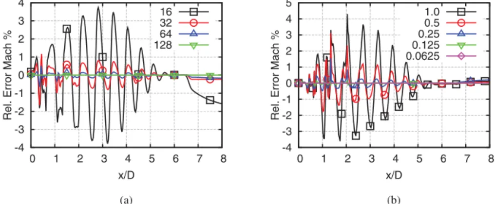
Inuncertaintyquantificationitisnecessarytohaveaconverged meshforalldeterministicsimulations.Thisrequirementis particu-larlyimportantforflowscontainingshocks.Inthisunder-expanded jet, the shock-cells are actually a series of expansion and com-pressionwavesthatlooklikewiden shocks.Theabovementioned mesh has been thoroughlytested and obtainedwith the follow-ingconvergenceprocedureusingasreferenceparametertheMach number profile at the centreline for the deterministic base case andconditionswitha higherNPR. First,the meshhas been con-verged azimuthally with 64 cells, obtaining a relative error with respecttoarefinedmeshoflessthan0.15%asshowninFig.2(a). Second, the axial discretization is taken into account by varying the starting position where the mesh topology is uniform. Axial convergenceisobtainedwithan errorof0.2%withrespecttothe

Fig. 1. Mesh cuts representing every fourth cells in the plane (a) z/D = 0 and the plane (b) x/D = 0 .

Fig. 2. Mach number profile relative error of the deterministic base case at the centreline for (a) different azimuthal discretizations, where each line represents the number of azimuthal nodes, and (b) different axial discretizations, where each line represents the starting position where the mesh is uniform. The refined mesh has been used as converged solution.

mostrefinedmeshforthepositionof0.25DasshowninFig.2(b). Relativeerrorsofthesameorderofmagnitudeareobtainedforthe axialvelocityatx/D=1.Finally,they+_{hasbeencheckedsothatit}

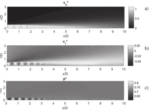
still laysintherangesmallerthanunityfortherangeofworking conditionspresentedinSection3.1.Contourplotsofthe determin-isticbasecaseareshowninFig.3.

2.3. Numericalformulation

The full three-dimensional compressible Reynolds-Averaged Navier-StokesequationshavebeensolvedbyusingtheFinite Vol-umemulti-blockstructuredsolverelsA_{(Onera’ssoftware[13])and}

will be briefly explainedhere. The turbulencemodel used inthe computationsofthisworkistheone-equationSpalart-Allmaras (S-A)standardmodel[89].Theconvective fluxiscomputedusingan upwindapproachbasedontheRoe’sapproximateRiemannsolver

[76]. The scheme’s accuracy is increased by the use of either a secondorderMUSCLextrapolation[98]coupledwiththeminmod limiter ora thirdorder extrapolationtechnique [15]. Theimplicit system is solved at CFL=100 with a LU−SSOR algorithm with four sweeps [103]. In orderto accelerate theconvergence for all the conditions, a converged deterministic base case solution has beenusedasinitialsolution.Thenumericalingredientsconsidered in this study follow the recommendations regarding the simula-tions of subsonic jet flows using the RANS modelling shown in

[24].

2.4. Turbulencemodel

Intheliterature, itisgenerallyadmittedthat thek−

ω

turbu-lence modelgivesthebestresultsforjets. However,withrespect

to other turbulence models, the use of the one-equation turbu-lence S-A model can be useful andthe studyof its performance forjetflowscanbeofinterest.BymeansofUQ,anassessmentof theaccuracyofthesimulationcanbedone.Touseaone-equation approach is also an advantage since, in uncertainty studies, the number of deterministic simulations to run is usually large and becomes a cheaperapproach. It is well known [42] that the S-A model needsimprovementforsubsonicjet flowshowever,Huang etal.[42]alsoshowedthattheone-equationmodelisthesecond bestoptionafterthek−

ω

modelintermsofrelativeperformances whentestedinseveralsubsonicacademiccases.Moreover,theS-A model,givesthebestnumericalperformancebasedongridspacing required foraccurate solutions andy+ _{allowableat thefirst grid}

point off the wall.Thisis forsurea positive aspectofthe model forUQsimulationswhenchangesinuncertainparametersleadto changesintheboundarylayerthickness.Forsupersonicflowssuch astheoneofasupersonic jetinatransoniccrossflow[70],even though the S-A model gives the worst results in terms of sur-face pressure, it gives the best agreement with experiments for thelocationandstrengthofvorticalstructures.Goodagreementis alsofoundforasupersonicunder-expandedejector[12]anda su-personic under-expandedimpinging jet [4]forseveralturbulence modelsincludingtheS-Amodel.

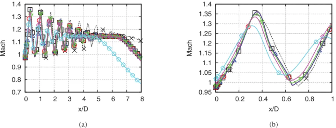
Nonetheless, differentturbulence models havebeentested for the base case to compare the validity of our choice. To this end, RANS simulations are performed with Fluent in the two-dimensional axisymmetric formulation.The Mach profiles at the centreline are shown in Fig. 4. Both codes give similar results for the S-A model interms of shock-cell spacingand amplitude, but Fluent resultsgive a shorterpotential core. The k−

ε

turbu-Fig. 3. CFD RANS simulations of the deterministic base case of the under-expanded jet in elsA . The shown parameters are (a) the dimensionless axial velocity, v∗

x = vx /c re f ,

(b) dimensionless radial velocity, v∗

r = vr /c re f and (c) dimensionless static pressure, p ∗=γre fppre f, with γ= 1 . 4 the specific heat ratio, p re f = 980 0 0 Pa the reference pressure and c re f = 340 . 26 m/s the reference speed of sound.

Fig. 4. Mach number profile of the deterministic base case at the axis for different solvers and turbulence models. (a) full view, (b) detailed view. Red dashed line: 3D elsA , S-A . Red solid line: 2D-axi Fluent S-A . Green solid line: 2D-axi Fluent k −ε. Purple solid line: 2D-axi Fluent k −ω. Symbols: Experimental data.

lencemodelgivessimilarshockspacingandamplitudeastheS-A model,butitcorrectlycapturesthepotentialcore.When compar-ing against theexperimental results, the turbulencemodel k−

ω

givesthebestresultsintermsofshockamplitude,butit overesti-mates thelength ofthepotential corebymorethan 50%.Similar decaysarefoundintheliteraturewhenusingdifferentturbulence models [1,28,80]. According tothese results,the Spalart-Allmaras modelhasa similarperformance thantheotherturbulence mod-els withtheadvantage ofhavingonlyone equation,andthus

be-ingnumericallymoreefficientandlesscomputationallyexpensive tosimulateseveralcasesforuncertaintyquantificationpurposes. 3. Uncertaintyquantificationon3DRANSsimulations

OneofthedrawbacksinRANS istoreplicateturbulence-based featuresreliably. Therefore,toquantifythe impactofinaccuracies inboth thecomputationalinjectionofturbulenceand experimen-tal jet performance is a plus. This provides extra metrics about theRANS simulation.ForthistaskUncertaintyQuantificationand SensitivityAnalysismethodsareapplied.Inthissection,theinput uncertainties are described aswell asthe mathematicalmethods usedfortheirhandling.

3.1. Testsandsourcesofuncertainty

Theparametersthat aretreated asstochastic inputsfor uncer-tainty quantificationare the stagnation pressure,ps, andthe tur-bulenttolaminarviscosityratio,Rt=

µ

t/

µ

,andarebothimposed at the inlet of the nozzle. These parameters have been selected becauseoftheir stochasticbehaviour innature.Other parameters could also be selected, butthese are the mostrelevant ones ac-cordingtoourexperienceandsomepreliminarytesting.

Oneofthegreatestsources ofuncertaintythat onecan recog-niseinthesejetflowsisthemass-flowrate,whichisinfactrelated toothervariablessuchasthenozzlediameterorstagnation pres-sure,beingthisflowparameteraninterestingandrelevantrandom inputtoreplicaterealisticconditions.Suchdecisionwas basedon suggestions ofexperimentalists atvon Karman Institute forFluid Dynamics (VKI),a partner in ourfunded project.During a single experimentalrun,notablepressurevariationsarenotyetexpected duetoemptyingofthetanks.However,theseareexpectedduring repeated tests. This is because the membranes of the valves are openingandclosingseveraltimes,andthedisplacementsofthese membranescanbeslightlydifferentforeachrun,leadingto varia-tionsinthemass-flowrate.Moreover,onehastotakeintoaccount theuncertaintyofthemeasurementdevices(pressuresensors).

Fig. 5. Mach number profile of the deterministic base case at the centreline for different R t inlet values in a (a) general and a (b) detailed view. Experimental × , R t =

0 . 022 ¤, R t = 0 . 22 , R t = 2 . 2 , R t = 22 , R t = 220 , R t = 2200 .

Fig. 6. R t profile of the deterministic base case at the centreline for different R t inlet values in a (a) general and a (b) detailed view. R t = 0 . 022 ¤, R t = 0 . 22 , R t = 2 . 2 ,

Rt = 22 , R t = 220 , R t = 2200 .

Asthetestrigwasnotyetbuilttomeasurethestagnation pres-sure(ps)uncertainty,itwasagreedwiththeexperimentaliststoset a realisticrangeto computethe inputuncertaintyby a conserva-tivevariationofa ±5%bymeansofauniformprobabilistic distri-bution.Theaimis,therefore,alsotogainusefulinformation,prior the first experimental test at VKI, by means of simulations. The sameconservativeapproachwasfollowedforthesecondsourceof uncertainty,thelaminarviscosityratio(Rt),whoseuncertaintywas testedcomputationally.Tosumup,thechosenprobabilistic distri-butionisps∼U

(

0.95¯ps,1.05¯ps

)

=U

(

211337,233583

)

Pa,where ¯ps refers to the deterministic base value ¯ps=222,460Pa. For nota-tion purposesinthispaper,the variationcoefficient from0.95to 1.05willbealsoreferredtoascps.

Asaforementioned,thesecondparameteristhelaminarto tur-bulent viscosity ratio, Rt=

ν

t/

ν

, used for the injection of turbu-lence intheSpalart-Allmarasmodel [89],whichisin facta com-putationalinput fortheturbulenceattheexitofthenozzle.This ismorecomplicatedtohandlethanthestagnationpressure,since thereisnoexperimentalbenchmarkdataavailableforacalibration process, because thisis a purely numerical.This parameter stays fixedwhensimulatingtheoperatingconditionsofanexperimental facility.However, dealingwithitasadeterministic fixed parame-ter is notappropriate, asflow simulationsare definitely sensitive totheirsetvalueandtoquantifythechangeinthesimulationsis relevant.Thevariationoftheparameterhasbeencarefullychosen based on several testson the CFD solver, forwhich the solution is closeto subsonic experimental results(used asguidance since therearenosupersonic experimentaldataavailable)evenwhenit islargelyvaried.

According tothebest practicesproposed by Spalartand Rum-sey[90],effectiveinflowconditionsfortheparameterRtshouldlie within therange(1,10). However,simulations withhighervalues

still give accuratepredictionswhileincreasing theconvergenceat highReynoldsnumbers.

Thislackofexactnessindefiningthisparameterencouragedus to deal withitasan uncertainty sourceby meansof an uniform probabilistic distribution.The CFDturbulent modelling by means ofthisparameterisnotlinkedtoanycompulsoryparticularorder of magnitude of this variable, andthis freedom provides a very wide rangeof valuesthat are almost equally validwithout prior knowledge. Thismightseema broadestimation,butthe prelimi-narytestssupportedtheidea.Thechosenprobabilisticdistribution isRt∼Unif(2.2,220)whereRt=2.2isconsideredthedeterministic basevalueasthiswasthevalueusedbytheauthorsinthe initiali-sationoftheflowforaLargeEddySimulation[9].Smallervaluesof Rtresultinchangesintheinjectionofturbulencetoosmalltohave an effect on the flow. On the other hand, by increasing this pa-rameterattheinlet,itincreasesalsothemaximumdimensionless turbulent wallunit,y+_{,achievedatthewall neartheexit.}

Never-theless,they+_{remainsoforderunitychangingfrom1to6forthe}

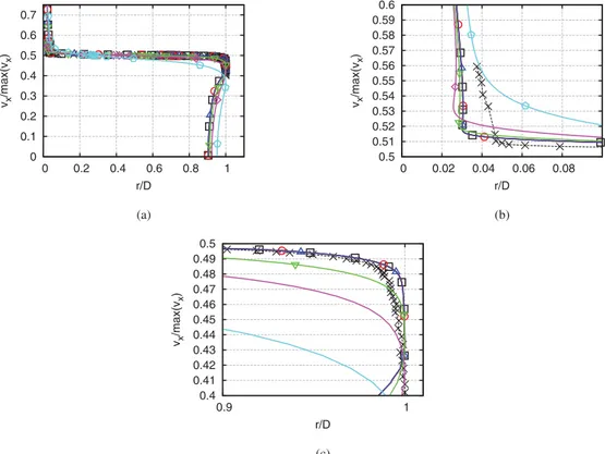
highestRt value.Figs. 5and6showthe MachandRt profiles for different Rt inletvalues,respectively. Values greaterthan 220are notpartofthestudyastheypresentnon-physicalvelocityprofiles asshowninFig.7fortheaxialvelocityprofileatx=2mm,which arecomparedwiththeavailableexperimentaldata.Thevaluesare non-dimensionalisedbythemaximumvaluesduetothefactthat the experimentaldata correspondsto asubsonic testcasewitha MachnumberattheexitofthenozzleofMe=0.9.

Other random inputswere discarded.Feasible parameters suf-fering fromuncertaintymightbeflowtemperatureorgeometrical variations suchasthediameterofthenozzle.Nevertheless,in or-dertonoticesomeeffectonthesimulations,thesevariationsmust be remarkablygreater thanthe expectedvariationeffect(at least oneorderofmagnitude).Otherprobabilisticdistributionscouldbe

Fig. 7. Axial velocity profile of the deterministic base case at the centreline for different R t inlet values in a (a) general and a (b) & (c) detailed view. Experimental × ,

Rt = 0 . 022 ¤, R t = 0 . 22 , R t = 2 . 2 , R t = 22 , R t = 220 , R t = 2200 .

tested too.However, asthemain goalis to beconservative prior any experimental testsat VKI and be aware ofpossible relevant variations inthequality ofthejet flowcomputation,the uniform distributions werethebestchoice.Thismodellingsuggest thatall inputsareequallylikelytohappen.

3.2. Uncertaintyquantificationmethods:generalisedpolynomial chaosandKrigingsurrogates

Uncertainty quantification (UQ) has become a very influential field, dueto thefact that methodsdeveloped intherecentyears bring the possibility of understanding how the behaviour of ex-pensive (normallyintermsofcomputation)mathematicalmodels isbeingaffectedbyimpreciselydefinedinputs.Foramoreformal description, letconsider thedifferential operatoron an outputof interestofastationaryproblem,y(x,

ξ

(

η

))as

L

(

x,

ξ

(

η

)

;y

(

x,

ξ

(

η

)))

=Q

(

x,

ξ

(

η

))

, (3) withLandQthedifferentialoperators onD×

4

,wherex∈D⊂ Rd_, d∈{1, 2, 3}.

η

denotes events in the complete probabilistic space

(

Ä

ˆ,Fˆ,Pˆ

)

,with Fˆ⊂2Ĉ the

σ

-algebra of subsets of

Ä

ˆ and

ˆ

Paprobabilitymeasure.

4

⊂ RNξ_{,isthestochasticspaceonwhich}

therandomvariables

ξ

(

η

)aredefinedandN_ξ standsforthe num-berofrandomvariables(twoinourcaseunderstudy).

The first approach presentedin thissection is thePolynomial Chaosmethod.ThismethodhasbeendevelopedtosolveStochastic Differential andStochastic PartialDifferentialEquations (SDE and SPDE, respectively) [91].It was first introduced by Wiener [104], in order to model stochastic processes through Hermite polyno-mialswithGaussianrandomvariables.Lately,XiuandKarniadakis extended the originalversion of Wienertoa wider familyof ba-sis functionsleadingtotheknownconceptofgeneralized Polyno-mialChaos(gPC)[107].ItisalsoknownasAskey-Chaos,duetothe fact thatisformedby thecompletesetoforthogonalpolynomials fromtheAskeyscheme[10].Theobjectiveofsuchextensionisthat

fornon-Gaussianrandominputs,theconvergenceofthe Hermite-chaosislow,andinsomecases,disastrous.

PolynomialChaosisaspectralmethod.Thus,an important ad-vantageisthat onemaydecompose arandomrepresentationinto deterministicandstochasticcomponentsas

ˆ ygPC

(

x,

ξ

)

= ∞ X j=0 ymj

(

x

)

9

j

(

ξ

)

, (4)

whereym_j arethedeterministiccoefficients(alsocalledmodal co-efficients) with x=

(

x,r

)

and

9

j(

ξ

) is the orthogonal base, in a tensor-like form by 1-D products of the orthogonal polynomials, satisfyingtheorthogonalityrelation

­

9

i,

9

j

®

=

­

9

i2

®δ

i j, (5) with

δ

ijtheKroneckerdeltafunctionand

h

·, ·

i

theinnerproduct. InEq.(4),theexpansion hasinfiniteterms.Forpractical reasons, thisexpansionhasto be truncatedaccountingNt−1terms,with

Nt=

(

Nξ+P

)

!

Nξ!P! (6)

andPstandingforthemaximumorderoftheexpansion.Thechaos expansionisfinallyexpressedas

ˆ ygPC

(

x,

ξ

)

= Nt−1 X j=0 ymj

(

x

)

9

j

(

ξ

)

. (7)

Inthefollowing,xand

ξ

areremovedinthenotationforsakeof simplicity.PolynomialChaoscan bean IntrusiveorNon-Intrusive approach.InthispaperitisimplementedasNon-Intrusive,dueto thefactthatittakesintoaccountthesolverasablack-boxnot re-quiringtocode insidetheCFD software.Thishasbeena popular methodin recentyears withmany successfulapplications in the literature[17,27,53].Astheinputuncertaintieshavebeenmodeled by Uniform ProbabilisticDistributions, Legendre polynomial basis

functionsarechosen.Forthedeterministicrealisationsrequiredin the expansion, collocation points have to be carefullyselected if one wantstoreduce thenumberofmodelevaluations.Regarding theselectionofthecollocationpointconfiguration,theuseof ten-sor grids represents an expensive way.A much efficientmean is the use of sparse grids [87]. In thiswork, Clenshaw-Curtis (C-C) quadraturenestedruleisapplied[99]togeneratetheweightsand nodes of the sparse grid. The coefficients ym_j can now be com-putedas ymj=

­

y,

9

j

®

­

9

2_j

®

. (8)

TheevaluationofEq.(8)isinfactthecomputationofthe mul-tidimensionalintegraloverthedomain

Ä

ˆ,onwhichdeterministic simulations of y from the CFD solver are set by the sparse grid. Moreover, thisinner productis basedonthe measureof weights according to thechoice of the orthogonal polynomials

9

, asthe weightfunctionisinfacttheprobabilisticdistributionfunction.As input uncertaintyis modelledby uniformdistributions, the spec-tralmethodturnsintoaPolynomialLegendreChaos.Oncethe co-efficients arecomputed, themeanandthevariance canbe found by E

₍

yˆgPC

₎

_=y m0, (9) V

(

yˆgPC

₎

₌ Nt−1 X j=1 y2mj

­

9

2_j

®

. (10)

An advantage of Polynomial chaos is that Sensitivity Analysis is straightforwardfromUQanalytics. ThisisdiscussedinSection4.

The second approach is Kriging interpolation (also known as Gaussian Processregressionandinthispaperundertheacronym KG).Thismethodisaninterpolationsurrogatemethodto approxi-matesetsofdata.Despitethefactthatsurrogatescanbealso con-structed via Polynomial ChaosExpansion,the main idea ofusing Krigingistotryanothermethodforcomparisonpurposes.Itisalso possiblehencetotestwhetherKrigingsurrogatescanhavea reli-ablebehaviourwithonlyabudgetof65deterministicsimulations fromcollocationmethods.

Inessence,Krigingisatwo-stepprocess:firstaregression func-tionf(

ξ

) isgeneratedbasedonthedataset,andfromitsresiduals aGaussianprocessZ(

ξ

)isbuilt,ascanbeseeninEq.(11)

ˆ yKG

₍

_ξ

₎

_{= f}ˆ

₍

_ξ

₎

_+Z

₍

_ξ

₎

₌ k X i=1

γ

ifi

(

ξ

)

+Z

(

ξ

)

, (11) where f(

ξ

) stands for the k×1 vector of basis regression func-tions [f₁

(

ξ

)

f₂

(

ξ

)

. . .f_k

(

ξ

)

] and

γ

i denotes the coefficients. De-pending on the regressionfunction, Kriging canappear with dif-ferent names. Universal Kriging defines the trend function as a multivariate polynomial, as described in Eq.(11). Simple Kriging refers to the use of a known constant parameter as regression function,i.e. f

(

ξ

)

=0.AmorepopularversionisOrdinaryKriging, which also assumesa constant but unknown regression function f

(

ξ

)

=

γ

0. Universal Kriging with a second order polynomial

re-gressionwasourchoice.

The Gaussian process Z(

ξ

) is assumedto have meanzero and co

v

(

Z

(

ξ

_i

)

_,Z

(

ξ

′

i

))

=

σ

p2Rc

(

θ

,

ξ

i,

ξ

i′

)

, where

σ

p2 is the process vari-anceandRc

(

θ

,

ξ

i,

ξ

i′

)

isthecorrelationmodelorspatialcorrelation function (SCF).In ordertocreatean accurate Krigingsurrogate it isimportanttopayattentiontothecorrelationfunction.This func-tiononlydependsonthedistancebetweenthetwopoints

ξ

iand

ξ

′

i, and, for the generalexponential case introduced in Eq. (12), alsoonp.Thesmallerthedistancebetweentwopoints,thehigher thecorrelationand,hence,themoretheKrigingpredictoris influ-encedbytheother.Bythesametoken,ifthedistanceisincreased,

thecorrelationdropstozero.Forthesereasons,itisnotusefulto putseveraldatapointstogether,asthepredictionwouldnotbe in-fluenced. Manycorrelationscan betried, butinthepresent work the generalized exponential worked very well and was the final choice.FromEq.(12),exponential(p=1)andGaussian(p=2) cor-relations were not appropriate forthe wave-like surrogates since during teststheseshowedsome bumpedareas inthe spaces be-tweencollocationnodes.

Rc

(

θ

,

ξ

i,

ξ

i′

)

=e−θ |ξi−ξ

′

i|p (12)

Theessentialdifferencebetweenthetwomethodssuggestedin thispaperisthatwhilst gPCestimatesthecoefficientsforthe or-thogonalpolynomialbasisfunctionschosenaccordingtotheinput distributions,Krigingisassumingthattheoutputoftheblack-box model due to input variable uncertainty behaves as realisations of aGaussian random process.This Bayesianapproach intendsto find probabilistic distributions over the functions, which are up-dated fornewobserveddata.TheGaussiandistributions also per-mittocomputeempiricalconfidenceintervalsthatprovidea guid-ance onthepositionswhereonecouldputadditionaldatato im-prove the fit. When applying Kriging, it is assumed that data is spatially autocorrelated andstatisticalpropertiesare independent on exactlocations[45].Krigingisnot an efficientchoice fordata with veryabrupt changes ordiscontinuities. Forfurther informa-tiononKriging(Gaussianprocesses),thereaderissuggestedtosee

[18,74]. Toapply the method,functions fromthe Matlab toolbox DACE[52]havebeenused.

Since shock-cells could createwavy changes insome features, the generation of surrogates has been carefully tested. The best performance wasobservedforthegeneralexponentialcorrelation, whose resultsforcomplicateddata setsat differentx/D locations to be interpolatedcanbe seeninFig. 8.Notethat thesurrogates have anon-sharpshape, soit isnot expectedtohavesubstantial erratic contributions inuncertainty quantificationwhen sampling acrossinternodalareas.

Oncethe Krigingsurrogates areavailable, samplingtechniques are affordable. Latin HypercubeSampling[39] andRandom Sam-plingMonteCarloarewidelyusednon-intrusivemethodsfor prop-agation ofuncertaintyinmodels. Thesemethods havebeenused formanyapplicationsinscienceandavastliteraturecanbefound. Because of the more stratifiedsampling, Latin Hypercubeis pre-ferred inthiswork.InSections3.3and4,theapplicationof sam-pling techniques andSensitivityAnalysis on Krigingsurrogates is developed and a comparison betweenKriging and gPC results is discussed.

3.3. Comparisonanddiscussionofuncertaintyquantificationresults The first stepforuncertaintyquantification istotest the con-vergence of each method with our computational budget. The ideabehindusingtwodifferentmethodswithdifferentprocedures (Kriging surrogatebysamplingandgPCbyquadratureon colloca-tion points)isto providetwo differentwayshopefullyleading to the sameconclusions. When focusingon morethan one method, conclusionscanbecontrasted.Ifasecondapproachisgiving simi-laroutputs,amorereliablefeedbackisprovided.

Forthispurpose,severalsamplingsweretriedonKGsurrogates byLatinHypercubeSampling(LHS)andtheresultswerecompared withthegPCexpansionof4thorder(asN_ξ=2,only21termsare requiredintheexpansion).Theaccuracyofthemethodshasbeen testedalongtheliplineforthedimensionlessaxialvelocity,

v

∗_x,and

along the centrelineforthe Machnumber, asthesearethe most relevant parts ofthe jet (alongthe centreline the shock-cells are strongandpreliminarytestsrevealedthatthenozzleliplinecould have a sensitive part for

v

∗_x variations).To compute the integrals

Fig. 8. Examples of Kriging surrogates at several x / D distances on data sets with challenging shape. The points correspond to the deterministic CFD solutions from the fourth level of accuracy in the Clenshaw-Curtis sparse grid. In the plots c ps stands for the coefficient of variation for p s ( ± 5%). (For interpretation of the references to colour in this figure legend, the reader is referred to the web version of this article.)

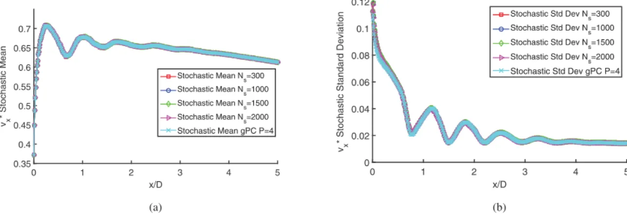
Fig. 9. Evolution of the v∗_{x stochastic means (a) and standard deviations (b) along the lipline for LHS on Kriging surrogates with different number of samples, N} s , and its

comparison with gPC results. Even for a small number of samples, LHS is undergoing very good convergence.

points based onClenshaw-Curtis (C-C) nestedrulewas used (the 65 collocation points correspond tothe fourthlevel ofaccuracy), having a good matchwith Kriging sampled surrogates as shown in Figs. 9and10.The requirednumber ofcollocation points was tested in[36],computingthe convergenceof statisticalmoments withStochasticCollocationMethod,sothatlevelofaccuracyofthe sparsegridwasintendedhereforgPC.

ForconvergenceofgPC,theorderofthe expansion,P,andthe number of collocation points, Nq, have to be controlled. If Nq is fixed to the fourthlevel of accuracy (lvl4) as aforementioned, it is now necessary to focus on the order of the expansion, P, to

compute the statistical moments. These undergoconvergence up to P=4. However, if P>4, divergence occursand this is due to thefact that morecollocation points are needed tocompute the integrals.This hasbeen testednumerically by means of generat-ing artificial deterministic solutions from Kriging surrogates (see

Fig.11andTable1).Withthisprocedure,theadditional determin-isticsolutions of the sparse grid required forthe fifth andsixth levelofaccuracy(lvl5artifandlvl6artifinthelegendoftheplots) are artificiallygenerated andhigher orders inthe gPC expansion aretested. Theseplotsare revealingthat,infact,inthe regionof 3<x/D<4morecollocationpoints wouldberequiredwithhigher

Fig. 10. Evolution of the Mach stochastic means (a) and standard deviations (b) along the centreline for LHS on Kriging surrogates for different number of samples and its comparison with gPC results. Even for a small number of samples, LHS is undergoing very good convergence.

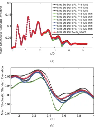
Fig. 11. Evolution of (a) Mach stochastic standard deviation for different P and lev- els of the sparse grid and (b) a zoom of the hardest part in the convergence anal- ysis. These results are compared with Kriging surrogates sampled by means of LHS with N s = 20 0 0 .

P.Asforlvl5andlvl6arerequired145and321collocation points respectivelywithanotveryrelevantimprovementintheaccuracy, it is not worthy to perform such a large number of simulations withtheCFDcodeandlvl4isassumedtobeenough.Moreover,an adaptiverefinementmethod[106]wouldnot beworthysincethe surrogatesaredifferentateachpointofthedomain.

Regarding the convergence ofsampling on Kriging surrogates, evenwithareducednumberofsamples,convergedstatistical mo-mentscanbeobtained.ThisisbecauseLHSisasamplingstrategy moreefficientthanMonte-Carlo andalsoduetothefact thatthe stochasticdimensionislow,requiringtosamplelessdimensions.

Forthepurposeofvisualisinguncertainty,thecontourplotsof the stochasticmean andvarianceare representedforboth

meth-Table 1

Since the initial budget was 64 points, and C –C sparse grid are nested, the additional collocation points for lvl5 artif and lvl6 ar-

tif are artificially generated from the Kriging surrogates. C-C level of the sparse grid Number of collocation points

lvl4 64

lvl5 artif 145

lvl6 artif 321

ods.InFigs.12,13and14thesevaluesareplottedfor

v

∗_x,

v

∗_randp∗

forKrigingsurrogates only.Theabsoluteerrordifference between KGandgPC isonlyshownfor

v

∗_x,sinceforall variablessuch

dif-ferenceisnegligible.Despitetheabsoluteerrorinthevariancecan seemslightlynotable,itisjustillustrative.Ifattentionispaidto

v

∗_x

alongtheliplineclosetothenozzleinFig.12d,theabsoluteerror seemstobenotable,butinFig.9thedifferenceispractically neg-ligible.The differencestakeplacebecausesurrogates aresampled withsamplesthatdonottakepartingPCanalysisand,ingPC, sta-tisticalmoments areobtainedby quadratureintegrals,andnotby samplingasinKG.

An objectiveofthe analysisistoassess thesimulationandto determinetheregions ofthejetpredictionwhicharemore sensi-tive totheinputuncertainties.Thespatialvariationinuncertainty isnotuniformacrossdifferentquantitiesofinterest.Diverse quan-titiesexhibitdiametricspatialsensitivitytoinputuncertainty.This hasbeensuspectedintheCFDcommunityforawhile[22],butno investigationhasqualitativeandquantitativeprofferedthisbefore. Fromacarefulanalysis,onecandrawthefollowingconclusions.

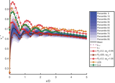
Forthe dimensionlessaxialvelocity,

v

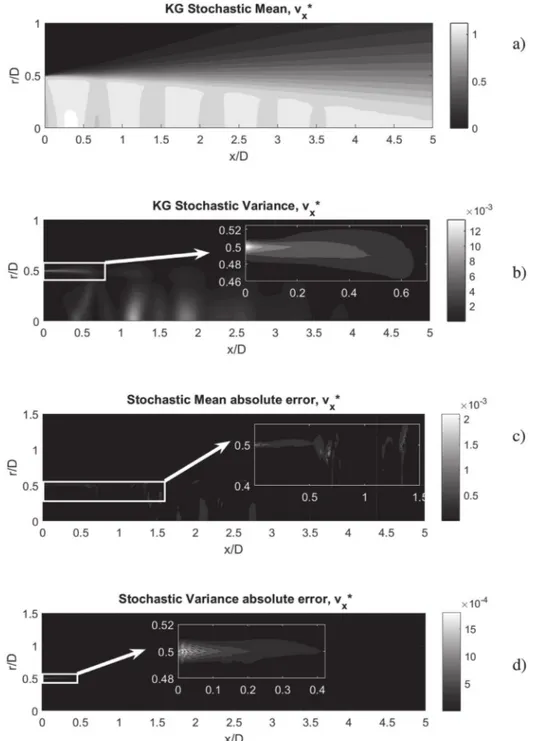
∗_x,themostsensitive re-gionisalongthelipline,closetothenozzlelip(seeFig.12b).This uncertaintyisinfacthigh,ascanbeobservedinFig.16.Suchlarge sensitivitynearbythenozzlelip makessense dueto thefactthat smallvariationsoftheinnerboundarylayerattheexitofthe noz-zle could potentially modify the features that take place in the nozzle lip/lipline regions. It is observed that the percentiles are slightlyfarfromtheS-Adeterministiccase.Thisdoes nothappen intheMachnumber(Fig.15),andtheaxialvelocityatthelipline seems to beaffected bythe Rt calibration(the deterministic case correspondstothelowestRtvalueintherandominput,being out-side theplottedpercentiles).Thisisactually obviousinthesense that the turbulencemodelhasa dramaticalimpacton the shear-layer. The computationunderuncertaintyremarks that fact:even ifRt ischosen wellenough accordingtothe Machnumberatthe centreline,theaxialvelocitycanbeunderestimated.Itis,thus, im-portanttolookattheliplineifexperimentalorbenchmarkdatais

Fig. 12. Contour plots of v∗_{x (a) stochastic mean and (b) variance by means of LHS on KG surrogates. Contour plots of the absolute error between (c) stochastic mean and (d)}

variance between KG and gPC methods.

availableforapropercalibration.Two-equationturbulencemodels dataandLES[9]areusedhereforcomparisonasthereisno exper-imentaldataavailableatthelipline,andonlyafterx/D=3thereis noticeabledifference betweenLESandS-Aresults.Tosupportthe observations,thetestswithRt fixedatitsdeterministicvalue and cpsvariedatitsminimumandmaximumareshown.Alsothetest when cpsfixed atits deterministicvalue andRt maximum.When Rtminimum,thatisthedeterministicsimulation(withlower val-uesofRt=2.2thevx∗doesnotchange).Itisguessedthatthe in-fluenceofthelargevaluesofRt withpsgeneratethelowervalues of vx∗.Also, whenps islarge, itis obviousthat the amplitudeof vx∗isincreased.

AgoodtestcouldbetotryalognormaldistributionforRt,and check howthe percentileplotchanges. However,since the

objec-tive ofthisworkis simplyto observethesensitivityunder equal probability (mostconservativecasescenario), itis discarded.It is recalled that in the initial seek for values for Rt, the jet perfor-mancewasslightlyperturbedforoneortwoordersofmagnitude in the change. In UQ applied to higher fidelity simulations (e.g. LargeEddySimulations,LES, not affordablehere)it wouldbe in-terestingto observewhethersimilar parametric uncertaintyfrom the computationof turbulence intensityhas an influence on the perturbationsintheshearlayerthatleadtothefeedbackloopfor screech noise [67]. Along the centreline, some uncertain regions canalsobedetected,butthesecanbebetteraddressedwhen de-scribingthevarianceinp∗_.

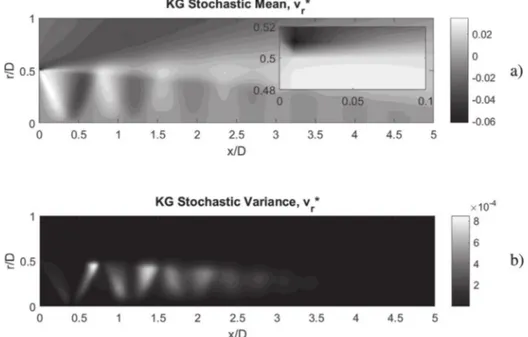
Regardingthedimensionlessradialvelocity,

v

∗_r,themost

Fig. 13. Contour plots of v∗_{r (a) stochastic mean with detail of the nozzle lip exit and (b) variance by means of LHS on KG surrogates.}

Fig. 14. Contour plots of p ∗_{(a) stochastic mean and (b) variance by means of LHS on KG surrogates.}

also be observed that the second and third shock-cell compres-sion are notoriously the mostsensitive to input uncertainty. Al-though jet noise is not studied in this paper because the avail-ablejetaeroacousticsmodelsarenotyetentirelyreliableinRANS, screechjetnoiseisusuallygeneratedinthatzone[66].

Forthedimensionlessstaticpressure,p∗_{,themostsensitive}

re-gionisalongthecentreline(seeFig.14b).Thisisalsoobservedfor the Mach number in Fig. 15, whereit can also be noticed some uncertaintyinthepositionoftheshocks.Thepercentileenvelopes showavariationinboththeamplitudeandpositionofthe shock-cell,whichmakessense duetothefactthatshockshaveastrong relationwiththevariationsinstagnationpressure,accordingto ba-sicfluiddynamicsofcompressibleflows.Theprescribed uncertain-tieswould, asexpected, be affectingthe robustness ofthe

simu-lated casescenario. In thisfigure, the percentile envelopes show that,despitethefactthattheCFDRANSwithSpalart-Allmaras (de-terministicsimulation) wasnotthemostaccuratemodel,the per-centile envelopes are able to cover the mostrelevant data (first four shocks-cell bumps). This is interesting, since RANS simula-tions struggleto undergoa good matchwithexperiments (espe-cially in high-speed flows with shocks andeddy-viscosity turbu-lence models). The non enveloped data are possibly not remark-ableoutliersifexperimentalerrorbarsareincluded(notreported in [5]). Inaddition,the changesintheposition oftheshock-cells arewell featured.However, itcanbeobservedthattheoscillatory patternisdissipateddownstream,asconsequenceofthevariations inthe shock-cellpositions(bumpeffectwiden)becauseof uncer-tainty sourcesandthedifficultyinRANSsimulationstoreproduce

Fig. 15. Percentiles from KG surrogates sampled by means of LHS with N s = 20 0 0 samples.

Fig. 16. Percentiles from KG surrogates sampled by means of LHS with N s = 20 0 0 samples. LES data from [9] .

arealisticjetpotentialcore.Itisinterestingtopointoutthateven LES data[9]hasproblemsto matchexperimental data,especially afterthethirdshock-cell.

4. Globalsensitivityanalysisbymeansofgeneralised polynomialChaosandKrigingsurrogates

4.1. Principleoftheglobalsensitivityanalysis

AsexplainedinSection1,anextensionofUQistheglobal Sen-sitivity Analysis. There are different methods for global Sensitiv-ityAnalysis, suchasScreeningMethod,DerivateBased Sensitivity AnalysisorVariance-BasedAnalysis[95].Thescientistmustchoose appropriately depending onthe computationalcost, dimensionof theproblemortheexpectedoutput,amongstothers.Forthe pur-poses of this work, a Variance-Based Analysis has been chosen

[77].One ofthe mainreasons ofusing thismethodis the possi-bility of ranking the influence ofthe input factors by sensitivity indices.

TheANOVAdecompositionofthevarianceisshowninEq.(13), and sensitivity coefficients are computed from Eq. (14) from its

proportionwithrespecttothetotalvariance.SiandST_i,inEq.(15), are the first-order and total sensitivity indexrespectively. In the followingequations themultiple subscriptsrefer tosecond, third or higher order interactions, depending on the number of sub-scripts. Given a model of the form y=yˆ

(

ξ

1,

ξ

2,...,

ξ

k

)

, with y a scalar,thedecompositionofthetotalvariance,V

₍

y

)

,canbe writ-tenas V

₍

_y

₎

= Nξ X i=1 V_ξ i+ Nξ X i=1,j>i V_ξ i j+ Nξ X i=1,k> j>i V_ξ i jk+... . (13)

The right hand side terms are the first andhigher order contri-butions to the total variance. Dividing by the total variance, the sensitivitiescanbecomputedas

1= Nξ X i=1 Si+ Nξ X i=1,j>i Si j+ Nξ X i=1,k> j>i Si jk +...+Si jk,...,Nξ. (14)

Thisleadstothefollowingexpresionforthetotalsensitivityindex forthei-thparameter

Fig. 17. Sensitivity indices contour plots by means of Kriging for p ∗_{. (a) and (b) are the first-order sensitivities and (c) higher-order interaction.} andtheassociatedsensitivitymeasure(first ordersensitivity

coef-ficient)iscomputedas

Si= V_ξ

i

(

Eξ∼i

(

y

|

ξ

i

))

V

₍

y

)

, (16)

where

ξ

i is thei-thfactorand

ξ

∼i denotes the matrixofall

fac-tors but

ξ

i.This indexindicates by howmuch one could reduce on averagetheoutput variance ifa parametercould be fixed.On theotherhand,thetotaleffectindexcanbecomputedas

STi=

E_ξ

∼i

(

Vξi

(

y

|

ξ

∼i

))

V

₍

y

)

. (17)

ST_i measuresthe total effect,i.e.first and higher ordereffects (in-teractions)offactor

ξ

i.Itrepresentsagoodmeasuretodetermine ifaparameterisinfluentialornot,andwhethercouldbeneglected fromthemodel.Theuseofthissensitivitytechniquecan beseen in many fields such as solar energy [81], wastewater treatment

[84]or heat exchangers[31].

AsthesensitivityindicesarerelatedtoUQ,theapproaches de-scribed inSection 3 are usedin thissection aswell. Particularly, theKrigingsurrogatesaresampledaccordingto[44]andthe coef-ficientsfromgPCare usedtocompute thesensitivityindices. De-spite that samplingcould also be done on the PolynomialChaos Expansion,it isimportant tonote that a second objectiveinthis work istohavetwo differentmethodologiestoachieve thesame results (sampling and quadraturebased approaches). It has been proceeded in this waydue to the fact that one of the interest-ing features of gPC isthe possibilityto perform Sensitivity Anal-ysisstraightforwardafteruncertaintyquantification.Forsuchtask, it is not difficultto realisethat thereis a clearrelation between

Eqs.(10),(13)and(14).Eq.(10)thatcanberewrittenas

1= 1 V

(

yˆgPC

₎

Nt−1 X j=1 y2mj

­

9

2_j

®

, (18)

andthe first andhigher-ordersensitivityindices cancarefully be extractedfromtheexpressionabove sincetheliteral partofeach monomialgivesthehintsoftheinteraction.

RegardingtheKrigingsurrogates,yˆKG_{,astheyareavailablefrom} theformeruncertaintyanalysis,itisnowpossibletocomputethe sensitivity indices from Eqs. (16) and (17). In order to compute S_i,

ξ

i hasto be fixed inseveral points

ξ

i=

ξ

i∗ along thepossible values of the random variable and compute the mean individu-ally for a further computationof V

ξi. This would require a very

large numberofcalculationssincethenumberoffixedpoints has tobe greatenoughtocompute reliablestatistics.Alessexpensive methodhasbeencodedinMatlabbyfollowingtheprocedure sug-gested in [44].With thismethod, the first ordersensitivity with Krigingsurrogates,SKG

i ,andthetotaleffect,SKGTi,canbecomputed as SKG i = 1−₂1_N s Ns P j=1

¡

ˆ yKG

₍

_B

₎

j−yˆKG

(

ABi

)

j

¢

2 V

₍

yˆKG

₎

, (19) SKG Ti = 1 2Ns Ns P j=1

¡

ˆ yKG

₍

_A

₎

j−yˆKG

(

ABi

)

j

¢

2 V

₍

yˆKG

₎

. (20)

In these expressions, yˆKG

₍

_A

₎

_{, yˆ}KG

₍

_B

₎

_{and yˆ}KG

₍

_AB

₎

_{are matrices} that contain model evaluations, product of decompositionof the original matrices whichcontain thesample campaign. Thesetwo original matrices, A andB, correspond to two different indepen-dentsamplesontothesamesurrogateandrandomvariables,with Ns×N_ξ dimensions.Eqs.(19)and(20)are builtupon theoriginal sensitivity indicesshowninEqs. (16)and(17).Thesenumerators comefromtheknownidentity

V

₍

_y

₎

₌V_ξ

i

(

Eξ∼i

(

y

|

ξ

i

))

+ Eξi

(

Vξ∼i

(

y

|

ξ

i

))

. (21)

Aformaldefinitionofthemethodrequiressomemathematical background in statistics andwill not be included in thissection. The reader isreferred to [35,44] forfurther details. However, for thesake ofpracticalclarification,theproceduredevelopedonthe surrogatesisbrokendownasfollows:

1. Generate two independentDesign of Experiment withLHS: A andB.

Fig. 18. Contribution to the total variance of (a) stagnation pressure, (b) laminar to turbulent viscosity ratio and (c) their interaction, for v∗

x .

Fig. 19. Contribution to the total variance of (a) stagnation pressure, (b) laminar to turbulent viscosity ratio and (c) their interaction, for v∗

r .

2. For the i-th sensitivity index, only the i-th column in matrix A isswapped withthei-thcolumninmatrix B.Thenew ma-trix is referred to as ABi_{. This new version of the A matrix} clearly preservesits Ns×Nξ structure andcan still be

consid-eredasamplematrix,butwithout theoriginalpropertiesofa LHS.

3. EvaluatetheKrigingsurrogateswiththeelementsfromthe ma-tricesA,BandABi_.

4. Compute the sensitivity coefficients in Eqs. (19) and (20). j standsfortherowofthematrices.

Thisalternativeapproachdramaticallydecreasesthenumberof modelevaluationsincomparisontobruteforcemethod.

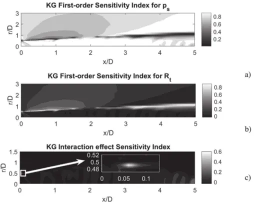
4.2.Discussionofglobalsensitivityanalysisresults

Sinceuncertaintyquantificationresultsarecomparedbymeans ofKrigingsurrogatesandPolynomialChaosinSection3,attention isnowpaidonthesensitivitycontoursforthedimensionlessstatic pressure,p∗_{,plottedinFig.17.}