Dynamique des glaciers vêlants et mécanismes de vêlage d'icebergs : le cas de Rink Isbrae, Groenland

DYNAl\IIIQUE DES GLACIERS VÊLANTS ET MÉCANISMES DE VÊLAGE D'ICEBERGS: LE CAS DE RINK ISBRJE, GROENLAND

MÉMOIRE PRÉSE TTÉ

COMME EXIGENCE PARTIELLE

DE LA MAÎTRISE EN SCIENCES DE LA TERRE

PAR

DOROTA MEDRZYCKA

Service des bibliothèques

Avertissement

La diffusion de ce mémoire se fait dans le respect des droits de son auteur, qui a signé le formulaire Autorisation de reproduire et de diffuser un travail de recherche de cycles supérieurs (SDU-522 - Rév.01-2006). Cette autorisation stipule que «conformément à l'article 11 du Règlement no 8 des études de cycles supérieurs, [l'auteur] concède à l'Université du Québec à Montréal une licence non exclusive d'utilisation et de publication de la totalité ou d'une partie importante de [son] travail de recherche pour des fins pédagogiques et non commerciales. Plus précisément, [l'auteur] autorise l'Université du Québec à Montréal à reproduire, diffuser, prêter, distribuer ou vendre des copies de [son] travail de recherche à des fins non commerciales sur quelque support que ce soit, y compris l'Internet. Cette licence et cette autorisation n'entraînent pas une renonciation de [la] part [de l'auteur] à [ses] droits moraux ni à [ses] droits de propriété intellectuelle. Sauf entente contraire, [l'auteur] conserve la liberté de diffuser et de commercialiser ou non ce travail dont [il] possède un exemplaire.»

Thank you, first of all, to my supervisor Mich 1 Lamothe. Michel, thank you for giving me the freedom to roam around and to complete this MSc program somewhat unconventionally, by spending most of the time away from Ivlontreal, either on Svalbard or in Sweden.

I also thank Doug Benn, my project supervisor. Doug it was a great pleasure to work with you and I truly appreciate your feedback. Thank you for taking me on fieldwork on Paulabreen and organising the Kronebreen fieldwork, I had the best time.

I want to thank all who helped during fieldwork: Nick Hulton for heading out with me to install the first cameras at Kronebreen, and Hcïdi Scvestre for retrieving the data and helping me out with all the small stuff afterwards. Thanks go to Jason Box for providing the new dataset from Rink Ibrœ after the Kronebreen cameras failed, and to both Nick Hulton and Doug Benn for coordinating the project. I spent quite a bit of time at Stockholm University (Institutionen for nat ur-geografi) where I was provided with access to a workspace (thank you Nina Kirch-ner) and plenty of coffee. Thank you to all at the department for your h lp. Special thanks go to the family and friends who provided me with plenty of dis-tractions in the form of additional fieldwork (Niels Weiss, Mark Allan), or trips (Niels Weiss, Ingeborg Pay, Mother and Father).

Funding was provided by the Fond de recherch du Québec - Nature et tech-nologies (FQRNT) and the Faculté des sciences de l'UQAM. Field expenses were covered by the Arctic Field Grant (AFG) of the Research Council of Norway (RCN).

This work has lead me to one major realisation: with any given project, nothing ever goes according to plan.

LISTE DES FIGURES . . LISTE DES TABLEAUX RÉSUMÉ . . .

INTRODUCTION CHAPITRE I

COMPORTEME TT DES GLACIERS VÊLA TTS. 1.1 Contrôles sur le processus de vêlage d'icebergs 1.2 Processus de vêlage d'icebergs . . . .

1.2.1 Taux de déformation longitudinale 1.2.2 Déséquilibre des forces au terminus 1.2.3 Vêlage sous-marin

CHAPITRE II

VARIABILITY IN CALVING BEHAVIOUR AT RINK ISBRLE, WEST V vu viii 1 6 6 g g 11 14 GREENLAND 15 2.1 Abstract . . . 15 2.2 Introduction . 15 2.3 Study site . . 17

2.4 Datasets and Methods 18

2.4.1 Timelapse cameras 2.4.2 Ice front mapping .

2.4.3 Calving event magnitude scale .

2.4.4 Surface air temperatures and Sea surface temperatur s 2.5 Results . . . . .. . .

2.5.1 Front position change 2.5.2 Air and sea temperature

18 19

20

21 22 22 23

2.5.3 Ice mélange clearing date

2.5.4 Event size distribution . .

2.5.5 Calving styles and calving front geometry

2.6 Discussion . . . . . . . . 2.6.1 Melt-driven calving . 2.6.2 Mechanically-driven calving 2.6.3 Ice mélange dynamics

2.7 Conclusion . CONCLUSION RÉFÉRENCES 24 25 27 37 37 39 41 45 47 50

Figure

0.1 Kronebreen, Svalbard . . .

0.2 Iordenskièildbreen, Svalbard

0.3 Camera et vue sur le terminus de Rink Isbrœ, Groenland

1.1 Champ de crevasses . . . . .

1.2 Schéma d'un front de vêlage

1.3 Kronebreen et Kongsvegen .

1.4 Schéma des forces au terminus

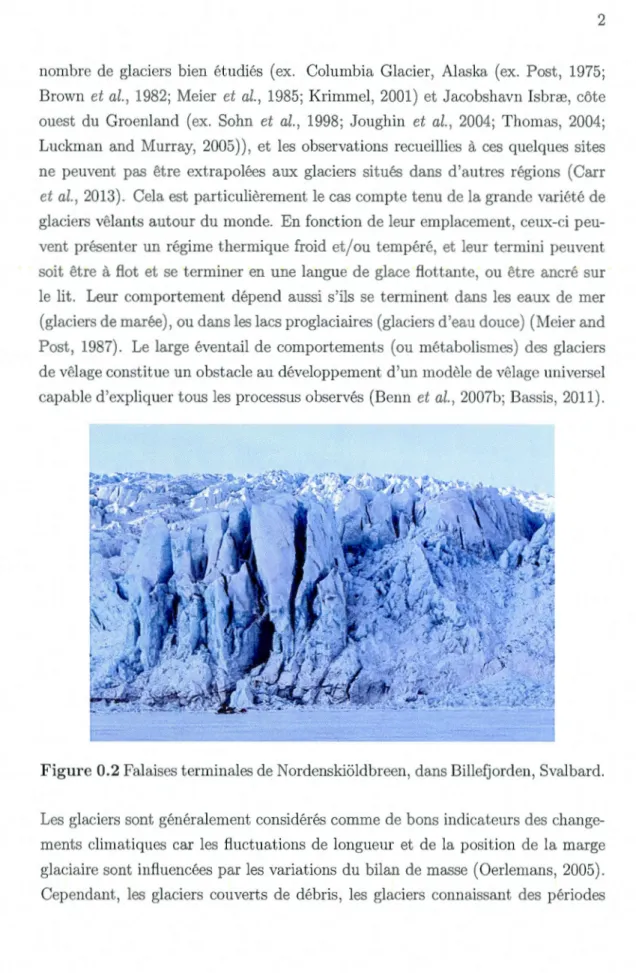
2.1 Study site

2.2 Grid . . .

2.3 Terminus position change.

2.4 Event size distribution and mass loss

2.5 Magnitude of daily calving losses for 2007 and 2008

2.6 Magnitude of daily calving losses: 2009, 2010, and 2011

2. 7 Magnitude of daily calving losses for all years

2.8 Spatial distribution of calving events

2.9 Pattern of surface crevasses . . ..

2.10 Calving front geometry after mélange clearing

2.11 Glacial meltwater upwellings

2.12 Notch at the waterline

2.13 Ice mélange . . . .. . Page 1 2 4 8 9 10 12 18 20 24 26 28 29 30 31 32 32 33 34 35

2.14 Magnitude 1 events . . . .

2.15 Calving pattern after mélange clearing

36

42

Tableau

2.1 Dataset

2.2 S asonal terminus position variations

2.3 Melt season and ice mélange clearing

Page

19

23 25

Le processus de vêlage, c'est-à-dire la production d'icebergs par les glaciers s'écoulant dans l'eau, est un mécanisme d'ablation important. Dans le cas des glacies de marée, et particulièrement dans le cas des glaciers situés dans les hautes lati-tudes, le vêlage entraine des pertes de masse bien plus importantes que l'ablation par la fonte seule. En dépit de leur importance évidente, les interactions dy-namiques entre le vêlage au terminus et les changements dans la dynamique du reste du glacier demeurent mal compris. Le présent mémoire traite de certaines questions concernant la complexité de la dynamique glaciaire des glaciers vêlants ("calving glaciers"), et examine la variabilité des processus de vêlage observés sur différents glaciers. Une étude de cas se concentrant sur Rink Isbrœ, un important glacier émissaire sur la côte ouest du Groenland, démontre qu deux styles de vêlage distincts agissent simultanément sur le même glacier. La variabilité dans le comportement de vêlage de Rink suggère que la production d'icebergs est le résultat d'une série de processus contrôlant l'ampleur, l'emplacement, ainsi que la périodicité des évènements de vêlage. La nature complexe des comportements de vêlage représente toujours un obstacle majeur à une évaluation précise de la sensibilité des glaciers de vêlage vis-à-vis les changements climatiques.

Les glaciers vêlants sont particuliers en raison du fait qu'ils se terminent dans l'eau et produisent des icebergs ce qui influence leur dynamique d'une manière fondamentale. La production d'icebergs est un mécanisme d'ablation dominant pour les glaciers de marée, et il est estimé être responsable d'environ 2/3 des pertes de masse de la calotte glaciaire du Groenland (Rignot and Kanagaratnam, 2006). Le vêlage représente donc une contribution majeure au flux d'eau douce vers les océans et joue un rôle clé dans les variations du niveau marin global (Rignot and Kanagaratnam, 2006). De nombreux glaciers vêlants, y compris dans l'Arctique, en Alaska, en Patagonie et en Antarctique, ont récemm nt connu une accélération rapide de leur écoulement, un amincissement et sont entrés en régression, résultant en une augmentation importante des taux de vêlage (ex. Arendt et al., 2002; Rignot et al., 2003; Cook et al., 2005; Rignot and Kanagaratnam, 2006; Bamber et al., 2007; Howat et al., 2008; Rignot et al., 2011).

Figure 0.1 Kronebreen, un glacier de marée s'écoulant dans Kongsfjorden, Sval-bard.

Malgré son importance évidente, la dynamique des glaciers vêlants et les mé-canismes physiques contrôlant le taux de vêlage restent toujours mal compris. L'état actuel des connaissances est limité par les défis associés à l'acquisition de données sur le terrain 'tant donné que les sites sont souvent situés dans des en-vironnements difficiles d'accès. La plupart des études sont menées sur un petit

nombre de glaciers bien étudiés (ex. Columbia Glacier, Alaska (ex. Post, 1975; Brown et al., 1982; Meier et al., 1985; Krimmel, 2001) et Jacobshavn Isbrre, côte ouest du Groenland (ex. Sohn et al., 1998; Joughin et al., 2004; Thomas, 2004; Luckman and Murray, 2005)), et les observations recueillies à ces quelques sites ne peuvent pas être extrapolées aux glaciers situés dans d'autres régions (Carr et al., 2013). Cela est particulièrement le cas compte tenu de la grande variété de glaciers vêlants autour du monde. En fonction de leur emplac ment, ceux-ci peu-vent présenter un régime thermique froid et/ou tempéré, et leur termini peuvent soit être à flot et se terminer en une langue de glace flottante, ou être ancré sur le lit. Leur comportement dépend aussi s'ils se terminent dans les aux de mer (glaciers de marée), ou dans les lacs proglaciaires (glaciers d'eau douce) (Meier and Post, 1987). Le large éventail de comportements (ou métabolismes) des glaciers de vêlage constitue un obstacle au dév loppement d'un modèle de vêlag universel capable d'expliquer tous les processus observés (Benn et al., 2007b; Bassis, 2011).

Figure 0.2 Falaises terminales de Nord nskioldbreen, dans Billefjorden, Svalbard.

Les glaciers sont généralement considérés comme de bons indicateurs des change-ments climatiques car les fluctuations de longueur et de la position de la marge glaciaire sont influencées par les variations du bilan de masse ( Oerlemans, 2005). Cependant, les glaciers couverts de débris, les glaciers connaissant des périodes

de crue, ainsi que les glaciers vêlants présentent souvent un comportement aty p-ique qui peut être dissocié des fluctuations climatiques. Les glaciers vêlants sont connus pour subir des cycles d'avancées lentes, suivies de retraits rapides dus à la désintégration du terminus par le vêlage (Post, 1975; Meier and Post, 1987; Post et al., 2011). Ce comportement instable suggère que la relation entre le vêlage et les forçages climatiques est complexe, et que la dynamique interne glaciaire ainsi que des facteurs spécifiques à chaque glacier ont une influence crucial sur les fluctuations de longueur des glaciers (Carret al., 2013). Comme décrit à l'origine par Post (1975), le cycle des glaciers de marée était considéré comme opérant sur des échelles de temps millénaires. Les avancées (rvl00-1,000 ans) et 1 s reculs ("' 10-100 ans) étaient donc traités comme une réponse (avec un certain délai) aux fluctuations climatiques à long terme (Post, 1975; Meier and Post, 1987). De nouveaux développements dans les deux dernières décennies ont abouti à une meilleure compréhension des conditions au terminus, c'est-à-dire l'interface entre l'océan et la glace, et ont révélé un couplage important entre les facteurs atmo-sphériques/océaniques, la présence de glace de mer au terminus, et la dynamique de vêlage (Carr et al., 2013). Des études récentes indiquent que les glaciers de marée peuvent subir des changements rapides sur des périodes courtes de quelques années, en réponse à un certain nombre de forçages environnementaux externes à court terme (Joughin et al., 2004, 2008b, 2012; Howat et al., 2007, 2008; Rignat et al., 2010; Straneo et al., 2010; Howat and Eddy, 2011; Nick et al., 2013). Le détachement d'icebergs est essentiellement un processus en deux parties impli-quant la propagation de fractures et la séparation de blocs de glace de la masse principale du glacier (Figure 0.2) (Bassis and Jacobs, 2013). Il est donc fortement couplé à la dynamique glaciaire et à l'équilibre de forces au terminus. La difficulté d'établir un lien clair entre les évènements de vêlage individuels et des facteurs déclencheurs spécifiques souligne la nature complexe des processus de vêlage. En d'autres termes, les évènements de vêlage peuvent résulter de multiples forçages agissant à la fois localement et globalement, et sur des échelles de temps courtes et longues (Benn et al., 2007b). Les contrôles potentiels affectant le comporte-ment des glaciers vêlants comprennent les facteurs spécifiques à chaque glacier, tels que l'épaisseur de la marge et la topographie du fjord, ainsi que les facteurs externes liés aux conditions atmosphériques et océaniques, autant locales qu'à

1 1

grande échelle. L'importance relative et les relations entre les différents forçages sont encore mal connues, et varient souvent selon le glacier et l'échelle de temps considérée. Cela pose un obstacle majeur à la formulation d'une évaluation précise de la sensibilité des glaciers vêlants aux changements climatiques (Bamber et al., 2007; Carr et al., 2013).

Figure 0.3 Camera et vue sur le terminus de Rink Isbrce.

Le présent mémoire se concentre sur cette question et examine le rôle des différents mécanismes qui contrôlent le moment, l'emplacement et l'ampleur des évènements de vêlage, afin d'améliorer notre compréhension des div rs mécanismes pouvant contrôler le comportement des glaciers de marée. Le premier chapitre présente une synthèse de la littérature actuelle sur le comportement des glaciers vêlants incluant les contrôles sur le vêlage, ainsi que la gamme de processus conduisant au détachement d'icebergs. Le second chapitre est une étude de cas, présentant la variabilité des comportements liés au vêlage observés à Rink Isbrœ, un important glacier émissaire sur la côte ouest du Groenland. L'étude utilise des données visuelles fournies par un système de caméra digitale (Figure 0.3) installée par Dr. Jason Box (Geological Survey of Denmark and Greenland, GEUS) dans le cadre du Extreme Ice Survey (EIS), et consiste en une analyse de l'activité au front du

glacier sur une période de cinq ans (2007-2011).

Ce chapitre sous forme d'article est présentement en préparation pour soumission à une revue scientifique, avec comme second auteur, Dr. Doug Benn (University Centre in Svalbard, UNIS), superviseur du projet de maîtrise duquel résulte ce mé-moire. Le chapitre, intitulé "Variability in calving behaviour at Rink Isbrœ, west Greenland" comporte une introduction détaillée au sujet traité. Les références pour tous les chapitres sont présentées ensemble à la fin du mémoire.

COMPORTEMENT DES GLACIERS VÊLANTS

1.1 Contrôles sur le processus de vêlage d'icebergs

La dynamique des glaciers vêlants est sensible aux conditions à l'interface entre la glace et l'océan dans lequel ils terminent. La présence d'eau au terminus influence l'équilibre de forces et a un impact majeur sur la résistance à l'écoulement à la base du glacier, et donc sur la vélocité de la glace, en particulier là où la profondeur de l'eau est suffisamment importante pour forcer le terminus à se soulever du à la poussée d'Archimède. Le terminus devient à flot si l'épaisseur de la glace est moindre qu'une épaisseur critique, ou l'épaisseur de flottaison, Hp:

Pw

Hp= - Dw

PI (1.1)

où Dw est la profondeur de l'eau et Pi et Pw sont la densité de la glace et de l'eau respectivement. Bien que la densité de la glace reste constante ("" 900 kg m -3_), la densité de l'eau varie (Benn and Evans, 2010). Cela signifie que l'épaisseur de flottaison est plus faible dans l'eau douce (Pw "" 1000 kg m-3

) que dans l'eau de mer (Pw "" 1,030 kg m-3) en raison de la différence de densité, dépendant de la salinité (Benn and Evans, 2010).

Le taux de vêlage d'icebergs, Uc, peut être défini comme la différence entre la vitesse à laquelle la glace est acheminée au front du glacier et le taux de change-ment de position du terminus:

-

oL

Uc =Ur

i_

où Ur est la vitesse moyenne d'écoulement de la glace, L est la longueur du glacier, et

t

est le temps (Benn et al., 2007a). Cette relation ente le taux de vêlage, l'écoulement de la glace, et la position du terminus peut être considérée de deux manières distinctes.

La première approche se concentre sur les contrôles sur les taux de vêlage t la vitesse de la glace, et les changements de position du terminus sont considérés comme le résultat d'un déséquilibre entre ces deux facteurs. Dans cette perspec-tive, le taux de vêlage est contrôlé par des variables environnementales indépen-dantes. Basé sur des observations sur un certain nombre de glaciers de marée en Alaska, Brown et al. (1982) ont proposé une connexion entre la profondeur de l'eau, Dw, au terminus et le taux de vêlage, Uc:

Uc

= a+bDw

(1.3)

où a et b sont tous deux des coefficients déterminés empiriquement (Benn et al., 2007a). Plusieurs études ont vérifié cette relation notant que le terminus devient instable lorsqu'il entre en contact avec des eaux profondes (Post, 1975; Pelto and Warren, 1991; Banson and Hooke, 2000; Skvarca et al., 2003). D'autres ont trouvé que ce modèle ne pouvait pas expliquer tous les comportements de vêlage observés étant donné que la relation entre le taux de vêlage et la profondeur de l'eau ne s'applique pas à tous les glaciers de marée et en tout temps (van der Veen, 1996, 2002).

La seconde approche se concentre sur la position de terminus et sur la vélocité du glacier et considère le taux de vêlage comme un résultat secondaire de la dynamique glaciaire (van der Veen, 1996, 1997b, 2002; Vieli et al., 2001, 2002). Meier and Post (1987) ont suggéré un lien entre le taux de vêlage et la pression effective (différence entre la pression de couverture de la glace, et la pression de l'eau à la base) à la base du glacier. Cette perspective prévoit que le glacier devrait se retirer vers une position où la pression effective à la base tend vers zéro et le glacier entre en flottaison. Van der Veen (1996, 1997b) a développé cette idée en incorporant la profondeur de l'eau et à proposé un nouveau critère qu'il a nommé "height above buoyancy". Ce critère suggère que le glacier a tendance à reculer vers une position où la hauteur totale du terminus atteint une valeur critique

( "'50 m) au dessus de son épaisseur de flottaison. Une variation à ce critère a été proposé par Vieli et al. (2001, 2002) où la valeur fixe de 50 m est remplacée par une fraction donnée de l'épaisseur de flottaison. Une limitation importante de ce critère est qu'il ne tient pas compte des platesformes et des langues de glace

flottantes, car il ne permet pas au terminus de s'amincir au delà de l'épaisseur de

flottaison sans se désintégrer en morceaux (Benn et al., 2007 a, b).

Figure 1.1 Champ de crevasses à Kronebreen, Svalbard.

Afin de répondre aux lacunes des modèles précédents Benn et al. (2007a,b) ont proposé un critère de vêlage basé sur la profondeur des crevasses qui prédit la position du terminus en considérant le taux de contraintes longitudinales près du front du glacier (Figure 1.1). Ce critère indique que le détachement d'icebergs se produit lorsque le régime extensif est suffisant pour que les crevasses puissent se

propager vers le bas, à travers la glace, pour atteindre le niveau de l'eau (Benn

et al., 2007a,b), ou, comme l'ont ensuite proposé Nick et al. (2010) pour que les crevasses se propagent à travers toute l'épaisseur du glacier. L'emplacement, la magnitude, et le moment du détachement d'icebergs dépendent donc tous de la propagation de fractures qui reflète l'état de stress de la glace, et qui dicte la position et la géométrie du front glaciaire.

1.2 Processus de vêlage d'icebergs

La propagation de fractures se produit en réponse à de multiples mécanismes de forçage, et le vêlage est probablement le résultat d'une série de processus (Fig

-ure 1.2). Benn et al. (2007b) ont identifié trois ordres de processus de vêlage capables de g'nérer des contraintes suffisantes pour provoquer la propagation de fracture et le détachement d'icebergs: (1) le taux de déformation longitudinale (ou l'allongement du glacier), (2) le déséquilibre des forces au front glaciaire, et (3) le vêlage sous-marin.

Figure 1.2 Schéma d'un front de vêlage et les processus opérant à l'interface entre la glace et l'océan (d'après W.T. Pfeffer, communication personnelle).

1.2.1 Taux de déformation longitudinale

La structure de vitesse d'écoulement du glacier est déterminée par la répartition spatiale des contraintes, notamment le "driving stress" et le "resistive stress".

Les gradients de stress longitudinaux s développent en réponse à la résistance au glissement, à la base du glacier et au marges latérales. La vitesse d', coulement a tendance à augmenter vers le terminus alors que le glacier devient à flot, du à

une réduction de la pression effective et une résistance au glissement moindre. La résistance au glissement est donc affectée par la présence d'eau au front, ainsi que par l'épaisseur du glacier. Ceci implique des vitesses plus élevées, plus la langue de glace est mince, et plus l'eau est profonde (Meier and Post, 1987; Vieli et al., 2000; O'Neel et al., 2001, 2005; Vieli et al., 2004; Howat et al., 2007, 2008). La résistance au glissement aux marges latérales est d'un autre côté inversement proportionnelle

à la largeur de la vallée glaciaire, et la vitesse a tendance à augmenter lorsque le

fjord s'élargit. Là où la résistance au glissement à la base est faible, la résistance

latérale peut contribuer de manière significative à l'équilibre des forces. Ceci peut

donc stabiliser le terminus et lui fournir la résistance nécessaire pour former un

langue de glace flottante (Benn et al., 2007a). Les gradients de str ss l

ongitudin-aux dépendent également des conditions aux falaises au front et au transfert de

"backstress11

• Van der Veen (1997a) définit le "backstress" comme le transfert, par

les gradients de stress longitudinaux, de la résistance à l'écoulem nt à la base et

aux marges latérale, vers l'amont du glacier. Là où les plateformes et les langues

glaciaires flottantes sont contraintes par la topographie, la perte d'un portion de

la glace flottante résulte en une réduction de "backstress" qui peut causer une

accélération en amont du terminus (Benn et al., 2007b). La structure de vitesse

du glacier dépend donc de la distribution spatiale de la pression effectiv , de la

largeur de la vallée, ainsi que des gradients de stress longitudinaux.

Figure 1.3 Kronebreen (bas gauche) et Kongsvegen (haut droit), Kongsfjorden, Svalbard. Les deux glaciers se joignent à 5 km du terminus t présentent des

régimes extensifs très différents. Kronebreen est fortement crevassé alors que

Kongsvegen a une surface plus régulière.

mélange de glace, ou 11

ice mélange11

, au front du glacier. Ce mélange de glace se forme en hiver et consiste en une masse semi-rigide formée de glace de mer et d'icebergs qui est poussé dans le fjord à la vitesse d'avancée du terminus. Le mélange agit essentiellement comme une mince langue de glace transitoire et peut générer un petite force résistive qui stabilise le front et limite le vêlage (Sohn et al., 1998; Joughin et al., 2008c; Amundson et al., 2010; Howat et al., 2010; Reeh et al., 2001; Herdes et al., 2012; Cassotto et al., 2015). Le vêlage reprend alors que le mélange s'affaiblit à la fin de l'hiver et diminue progressivement à la fin de l'été alors que la consolidation de la glace de mer résulte en l'accumulation progressive du 11

backstress11

(Sohn et al., 1998). La présence de glace de mer dans le fjord a donc une influence majeure sur la production d'icebergs et contribue aux avancées et reculs saisonniers (Sohn et al., 1998; Joughin et al., 2008c; Amundson et al., 2010).

Lorsque les contraintes d'extension sont suffisamment importantes pour initier le processus de fracturation, des crevasses transverses se propagent à travers la glace (Figure 1.3). De même, lorsqu'elles sont soumises à des forces supplé -mentaires, les crevasses préexistantes, advectées des régions de stress élevé en amont, peuvent aussi conduire au détachement d'icebergs (Bassis and Jacobs, 2013). L'introduction d'eau de fonte ou de pluie dans les crevasses de surface est un facteur additionnel pouvant renforcer la fracturation. L'action de l'eau a comme effet d'augmenter la pression dans les fractures et peut potentiellement forcer les crevasses à se propager à travers toute l'épaisseur du glacier ou de la plateforme flottante (van der Veen, 1998, 2007; Scambos et al., 2000; MacAyeal et al., 2003; Cook et al., 2012). Le taux de déformation longitudinale qui déter-mine l'emplacement et la profondeur des crevasses, ainsi que l'épaisseur de la glace au terminus qui décide de la facilité d'une crevasse à pénétrer jusqu'à la base du glacier, représentent ensemble le contrôle primaire sur les variations de position du terminus (Benn et al., 2007a,b).

1.2.2 Déséquilibre des forces au terminus

Le déséquilibre des forces agissant localement aux falaises de glace terminales représente un processus de second ordre, superposé sur la structure de vélocité du

Figure 1.4 Schéma des forces cryostatiqu s (gauche) et hydrostatiques (droite) au terminus. Un 11_backstress11 _{supplémentaire peut être fourni par la présence} d'un mélange de glace dans le fjord (modifié à partir de (Benn et al., 2007b)).

glacier. Les gradients de stress sont déterminés par l'interaction entre la pression cryostatique de la glace agissant vers l'aval, et la pression hydrostatique de l'eau qui pousse vers l'amont (Figure 1.4). En dessous du niveau de l'eau, la pression cryostatique est partiellement opposée par la force hydrostatiqu . C pendant, la partie subaérienne de la falaise de glace est pratiquement innoposée par la pression atmosphérique (Benn et al., 2007b). Les gradients de stress sont plus importants plus les falaises sont hautes, et la pression cryostatique augmente progressivement vers le bas pour atteindre un maximum au niveau de l'eau (Hanson and Hooke, 2000). Les contraintes extensives qui résultent de cette pression peuvent conduire à la propagation de fractures.

Le déséquilibre de force au terminus est potentiellement amplifié par l'érosion thermique résultant de la fonte au niveau, ou sous le niveau d'eau. La fonte sous-marine peut causer un surcreusement de la partie submergée et former un surplomb (Benn et al., 2007b). Bien que 1 taux de fonte augmente avec la tem -pérature de l'eau, le processus de convection induit par l'écoulement des eaux de fonte glaciaire vers le fjord joue un rôle crucial en renforçant la circulation sous -marine. La convection agit comme une pompe et assure l'arrivée des eaux marines relativement chaudes vers les falaises terminales, favorisant ainsi la fonte (Motyka et al., 2003, 2011; Jenkins, 2011). Lorsque les taux de fonte subaquatiques dé

encor le déséquilibre de force aux falaises de glace. Ceci conduit au bascule -ment vers l'avant de blocs de glace et éventuellement au détachement d'icebergs (Theakstone and Knudsen, 1986; Kirkbride and Warren, 1997; Vieli et al., 2002; Haresign and Warren, 2005). Dans certain cas, les taux de vêlag sont dir cte -ment contrôlés par la vitesse d'érosion thermique et de surcreusement des falaises terminales (Rohl, 2006; Dykes et al., 2010).

Les termini flottants sont aussi soumis à la force d'Archimède qui impose un torque sur la langue de glace à la jonction entre la section flottante et le reste du glacier sur terre. Un amincissement additionnel du terminus augmente le déséquilibre avec la pression hydrostatique et la glace devient à flot (Warren et al., 2001; Benn et al., 2007b). En raison de la différence de densité de l'eau, l'épaisseur de flottaison est plus élevée dans l'eau de mer que dans l'eau douce et, pour une épaisseur donnée, les glaciers de marée subissent une flexion supérieure aux glaciers lacustres. En réponse à la force d'Archimède, la langue de glace flottante peut devenir soulevée et inclinée vers l'arrière. La rupture se produit le long des lignes de faiblesse fournies par les crevasses préexistantes advectées de l'amont glaciaire (Benn et al., 2007b).

L'accroissement progressif des forces de flexion vers le haut peut être accommodé par la déformation interne de la glace, mais les perturbations plus rapides sont plus susceptibles de conduire à la propagation de fractures et au vêlage (Boyce et al.,

2007). Benn et al. (2007b) ont proposé que les taux de contraintes longitudinales sont le contrôle primaire sur la position du terminus car ils déterminent les limites de la marge glaciaire en déterminant l'emplacement des crevasses. Le déséquilibre de forces au terminus représente un contrôle secondaire car il sape davantage l'intégrité du front et peut causer le glacier à se retirer. Toutefois, lorsque les vitesses de déformation longitudinales sont faibles, la position du terminus peut être contrôlée directement par les processus secondaires. Malgré l'importance primordiale de la structure de vitesse du glacier dans le contrôle du processes de vêlage, il n'y a pas de relation directe entre les taux de déformation longitudinale et les taux de v'lage. Les processus décrits ci-dessus représentent les contrôles sur l'emplacement et la magnitude des événements de vêlage individuels, mais pas sur les taux de vêlage eux-mêmes (Benn et al., 2007b).

1.2.3 Vêlage sous-marin

Le vêlage sous-marin peut être considéré comme un contrôle de troisième ordre car il dépend des processus de premier et second ordre (Benn et al., 2007b). Les

sections submergées des falaises de glace, ou ce qu'on appelle des pieds de glace (''ice foot"), se forment en réponse à la fonte au niveau de l'eau, ou au vêlage de la partie subaérienne de la marge (Warren et al., 1995; Kirkbride and Warr n, 1997; Motyka, 1997; Vieli et al., 2002; O'Neel et al., 2007). La perte soudaine de la pression de couverture de la glace sur le pied de glace submergé entraine le déséquilibre des forces et peut causer le détachement de la partie sous-marine.

Les icebergs qui résultent de ce processus jaillissent vers la surface et émergent

VARIABILITY IN CALVING BEHAVIOUR AT RINK ISBR.!E, WEST

GREENLAND

2.1 Abstract

Iceberg calving is a sporadic process with a large variability in the magnitude, location, and timing of events. Calving styles range from the periodic breakup

of large full-thickness tabular icebergs from fioating ice tongues, to the more fre -quent capsizing of small blocks detaching above the waterline. The diversity in calving behaviours observed at marine-terminating glaciers points to the fact that iceberg production is the result of a series of different processes, and the precise

mechanisms responsible remain largely unknown. This study presents detailed ob-servations of calving behaviour variability from daily photographs acquired over a

five year period (2007-2011) over the terminus of Rink Isbrœ, west Greenland. The evidence suggests that calving at Rink is characterised by two distinct styles with

different temporal and spatial footprints. It is suggested that at least two (sets of) mechanisms are controlling calving variability at this location, namely (1) me lt-driven processes enhancing submarine undercutting and (2) mechanically-driven

buoyant flexure. As the second mechanism is responsible for most of the mass lost through calving at Rink, it could potentially represent an important control on the stability of other Greenland glaciers as well.

2.2 Introduction

Recent studies indicate that the dynamics of marine-terminating glaciers are se n-sitive to changes in boundary conditions at the terminus. Feedbacks between

calving and ice dynamics imply a strong coupling between processes acting at the

ice margins and changes upglacier (Joughin et al., 2004; Thomas, 2004; Howat et al., 2005; Joughin et al., 2008c; Nick et al., 2009; Vieli and Nick, 2011). Studies

focusing on individual calving events suggest that rapid and localised pertur ba-tions may additionally determine the location, magnitude, and timing of events (O'Neel et al., 2003, 2005, 2007; Bassis and Jacobs, 2013; Chapuis and Tetzlaff,

2014). Short-tenn terminus stability is therefore dependent on several parameters

modifying boundary conditions at the ice cliffs, including both atmospheric and oceanic factors, the presence of sea ice/ice mélange in the fjord, as well as glacier specific factors such as ice thickness and fjord bathymetry. For this reason, and

due to the wide range of calving styles observed at marine-terminating glaciers,

there is no universal law that would adequately explain all calving behaviour. The mechanisms controlling the variability in calving behaviour, including at the

interannual, seasonal, and single-event scale, remain largely unknown.

Calving is a sporadic process and consists of fracture propagation and the de -tachment of icebergs from the terminal ice cliffs following terminus destabilisation (Bassis and Jacobs, 2013). Calving styles and iceberg aspect ratio are therefore

primarily controlled by longitudinal stre s gradients within the glacier which de-termine the location and depth of transverse crevasses (Benn et al., 2007a; ick

et al., 2010). Variations in buoyancy conditions at the terminus further alter the

force balance and can push the ice margin out of equilibrium, and promote cal v-ing (Benn et al., 2007b). Several mechanisms have been proposed as having an impact on calving by modifying the force balance at the terminus. Longitudinal

stress gradients can be influenced by variations in backstress resulting from the

presence of a proglacial ice mélange in the fjord during the winter, which provides a small resistive force, stabilises the terminus and suppresses calving (Amundson et al., 2010; Vieli and Nick, 2011). Additionally, the presence of water in surface crevasses can promote calving by causing the fractures to deepen and produce icebergs (Benn et al., 2007a; Nick et al., 2010; Vieli and Nick, 2011; Cook et al., 2012). Buoyancy conditions can be affected by submarine melt and undercutting of the terminus which modifies the stress balance at the ice cliffs and promotes calving (Motyka et al., 2003; O'Leary and Christoffersen, 2013).

This study aims to identify the different mechanisms affecting calving behaviour variability at Rink Isbrœ, a major outlet glacier in west Greenland. Individual

calving events were documented from a dataset of daily terrestrial photographs acquired over the span of five years (2007-2011) by the Extreme Ice Survey (EIS). A qualitative assessment of calving behaviour was compiled including information

concerning the relative magnitude, timing and location of single calving events,

in order to determine the controls on event size, inter-event intervals, as well as any spatial patterns in calving activity. The temporal evolution of terminus ge-ometry indicates that Rink Isbrœ exhibits two distinct calving styles including

the sporadic detachment of large full-thickness km-sized tabular icebergs, and the more frequent capsizing of smaller bergs and slabs. The variability in ca lv-ing behaviour is shown to depend on the interplay between longitudinal stresses and buoyancy conditions at the terminus. More specifically, small events occur more frequently in response to melt-driven processes, whereas the large ones are

mechanically-driven and result from buoyant flexure at the terminus. 2.3 Study site

Rink Isbrœ (71°45'N, 51°40'W) terminates in a narrow fjord in the Uummannaq

district on the west coast of Greenland (Figure 2.1). With a drainage basin size

of 30,000 km2

, it drains rv3.53 of the Greenland ice sheet (Rignot and Kana

-garatnam, 2006) through a 4.5 km wide terminus. The front position remained

relatively stable over the 2000-2010 period (Howat et al., 2010; Box and Decker,

2011) and discharge rates of 11.8 km3 a-1 of ice were measured between 2000 and 2005 (Rignot and Kanagaratnam, 2006). No speedup or surface elevation changes were recorded between 2000 and 2009 (McFadden et al., 2011). Ice flow speed

variations are correlated with seasonal terminus position changes and surface ve -locities vary by approximately 253, ranging between 10 and 12.5 m d-1 _(Howat

et al., 2010).

Bathymetric data of the inner fjord reveals two deep basins reaching over 1000 m below water level, separated by a 200 m high submarine moraine ridge, peaking at roughly 600 m below water level, and extending across the fjord about 2 km from the ice margin (Dowdeswell et al., 2014). The maximum depth of the ice

at the glacier front is estimated to reach rv750 m in the midsection of the fjord (Chauché et al., 2014). Although there is no detailed data of ice thickness at the terminus, the fact that Rink Isbrœ produces large full-thickness tabular icebergs

indicates that the terminus may be close to floatation (Ahn and Box, 2010).

Figure 2.1 Study site. Left: Landsat 7 image (8 July 2014) of Rink Fjord on the west coast of Greenland. Green dots indicate the position at which sea surface temperature (SST) data was extracted around an 8 km radius, 10 (71°39.624N,

51°47.532W) and 40 (71°33.75'N, 52°54.048'W) km from the ice margin. Right:

Rink Isbrœ calving front with approximate viewshed of the camera marked by dashed red lines. Digitised ice front positions are shown for 2007 (yellow) and 2011(blue). The green reference box was used to calculate area changes between

successive Landsat scenes. The dashed blue line about 2 km down the fjord from the ice margin indicates the position of a 200 m high transverse submarine moraine

ridge.

2.4 Datasets and Methods

2.4.1 Timelapse cameras

A 10.2 M pixel digital single-lens reflex (SLR) camera (Nikon D200) with a fixed focal length lens (Nikkor 20 mm) was install don the southern sid of Rink Fjord

(71°42.348' r, 51°38.055'W) overlooking the calving front (Figure 2.1). The in-stallation was performed by Dr. Jason Box ( Geological Survey of Denmark and Greenland, GEUS) for the Extreme Ice Survey (EIS). A custom timer developed

by the US National Geographic Society's Remote Imaging Laboratory was pro -grammed to take daily photographs at 15:00 UTC between June 2007 and July 2011. The camera was enclosed in a Pelican case with a customs-installed opti -cally neutral plastic window, and powered with a 50 Ah gel cell battery connected to a 10 W solar panel. The lack of solar illumination during the polar night and camera malfunction in cold temp ratures resulted in data gaps of several months during winter. Additional data loss caused by clouds, fog, and rain drops ob-structing the view of the terminus accounts for a loss rate of rv 103 for all years of the study period (Table 2.1). In total 803 images were analysed for the entire study period.

Year Data period Days Yearly image Joss due to: Images clouds (%) other (%) analysed

2007 06.12-10.21 132 10.6 0 118 2008 02.15-10.06 235 10.6 0 210 2009 03.03-08.08 159 10.8 0.7 141 2010 03.31-11. 20 236 10.0 3.4 205 2011 01.28-07.21 182 11.0 19.8 129 Total 944 803

Tableau 2.1 Dataset, study periods and yearly image losses The high percentage of 'other' losses for 2011 are due to the fact that the camera remained operational during the winter (January-February) when cold temperatures ( <-30°C) caused temporary sticking of the shutter.

2.4.2 Ice front mapping

Calving front positions were mapped from Landsat 7 Enhanced Thematic mapper Plus (ETM+) band 8 panchromatic images with 15 m pixel resolution. Failure of the scan-line corrector (SLC) on the ETM+ and the resulting offset between scan-lines causes increasing data loss toward the scene edge where banding can reach a maximum width of approximately 400 m. About 153 of scenes were rejected due to significant portions of the front being lost. Useable cloud-free scenes provide data coverage of 3 images per month on average during periods of solar illumination (April-September) for a total of 12-20 images per year. Changes in ice front position between successive images were mapped following the method

described by Moon and Joughin (2008). Retreat and advance was measured using

a polygon, bounded on the downglacier side by the ice front which was manually

digitised and adjusted to fit the new front position on each successive image, and

three fixed lines: two on the si des approximating the lateral margins of the glacier, and one arbitrary line upglacier from the minimum observed front position (green

box in Figure 2.1). The average advance or r treat of the front was obtained by

dividing the difference in area of two polygons by the mean glacier width. This

method accounts for uneven front position variations along the glacier width and allows for a better approximation of advance and retreat as a linear distance.

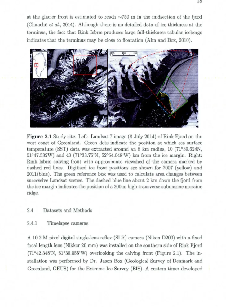
Figure 2.2 Left: Landsat 7 scene from 23 April 2010 with 500 x 500 m grid and

digitis d position of calving front. Right: Image taken on the same day (15:00

UTC) with approximate grid built based on the Landsat grid. The two red lines

indicate the front position before (22 April) and after (23 April) a magnitude 7

event. The size of the calved iceberg is estimated to 1.3 km2

2.4.3 Calving event magnitude scale

A total of 984 single calving events were documented following a semi-qualitative approach where the size and location of each vent was determined using an approximate grid overlaid over the terminus. The 500 x 500 m cells were built by comparing the location of easily identifiable features on select timelapse images

and the corresponding Landsat scenes acquired on the same day (Figure 2.2). The position of the calving front was manually digitised for each daily image

and the resulting sequence of vectors was analysed to identify variations in front geometry. Calving event sizes vary from small debris avalanches and isolated blocks detaching from the front, to large events involving nearly th full terminus

width. Events were classified following a non-linear magnitude scale ranging from 1 to 7 depending on their relative size. Th magnitude was attributed subjectively

for each event based on visual observation. The relative size of each event and

the associated mass loss were approximated based on the number of 500 x 500 m

cells implicated in the event.

Two distinct categories of events emerge from the data. The first consists of magnitude 2-7 events which are large nough to result in an effective retreat of a section of the front (i.e. the new front position is more retracted than the

previous one). The second category is made up of magnitude 1 events which

consist of debris avalanches and isolated blocks which alter ice front geometry but do not result in retreat. Due to the resolution of the images and the effects of

perspective, the method used can introduce a bias when it cornes to comparing

the relative magnitude of events occurring close to the camera, compared to those

happening on the other side of the fjord, 5 km from the camera. Small magnitude

1 events are especially difficult to identify at greater distance and under changing

light conditions due to different levels of cloud cover. The presence of ic mélange

in the fjord makes it difficult to identify the ice cliffs during winter/spring months,

or to pinpoint with precision the day an event occurs. Additionally, the dataset

for 2010-2011 was acquired by a different camera located about 100 m away from the first location. The view from the cam ra therefore changed for the last two years and the first 250 m or so of the front were obscured by rocks. Consequently,

the 2010-2011 dataset is missing some of the small events occurring close to the

southern margin.

2.4.4 Surface air temperatures and Sea surface temperatures

Sea surface temperatures (SSTs) were obtained from the Moderate Resolution Imaging Spectroradiometer (MODIS) instrument on the NASA Terra satellite.

Daily SST data series were extracted from the MOD28 product with 4.88 km

spatial resolution within an 8 km radius of two locations, 10 and 40 km down the

fjord from the ice margin (Figure 2.1). The presence of sea ice and ice mélange

cover influences temperature derivations and SST data is unavailable during the

winter months (January-March). Monthly mean surface air temperatures (SATs)

were extracted from measurements acquired every 12 hours by the Danish M

e-teorological Institute (DMI) at the Qaarsut Airport weather station (70°44'N,

52°42'W; 88 m a.s.l.), located in Uummannaq Fjord, 120 km south of Rink's ter

-minus (Cappelen, 2014). The number of positive degree-days (PDDs) was used as

a proxy for surface melt, and to determine the intensity and duration of the melt

season. Following the method used by Schild and Hamilton (2013), the onset and

the end of the melt season were taken as the first period of five consecutive days

where average temperatures were above, or below 0°C.

2.5 Results

2.5.l Front position change

The width averaged terminus position change calculated from Landsat imagery

(Figure 2.3) shows a seasonal variation with an average difference between the

annual maximum and minimum position of 670 m, corresponding to 3 km2 _across

the whole glacier front. The front typically reaches its seasonal maximum position

some time in June and the retreat lasts until the end of September and possibly

later, although the precise duration of the retreat phase is uncertain due to the

lack of visual data (both Landsat and terrestrial imagery) in late fall and winter.

Interannual data shows a relatively stabl terminus position with a slight retreat of

the seasonal maximum position of rv 750 m ( corresponding to a retreat of 0.8 km2

a-1) recorded over the study period. The amplitude of seasonal advance/retreat

also decreases by over half (from 950 to 360 m) between 2007 and 2011 (Table

Year l\!laximum position Minimum position Retreat phase Area loss Retreat ( day of year) ( day of year) (N days) (k1112

) (m) 2007 162 257 95 4.21 950 2008 126 210 84 3.11 660 2009 181 270 89 3.32 730 2010 167 259 92 2.58 590 2011 190 269 79 1.65 360 Average 165 253 88 2.97 658

Tableau 2.2 Seasonal terminus position variations at Rink Isbrce.

2.5.2 Air and sea temperature

Monthly mean air temperatures measured at Qaarsut over the study period are

highest in July (10°C) and lowest in March (-13.9°C). July temperatures show a slight increase of 0.34°C a-1 _{over the stucly periocl. The melt season generally} lasts from early May until late September with an average duration of 129 clays. With the exception of 2010, the year with the longest melt s ason, where positive

temperatures persist for 168 days until late October.

SST data is unavailable for the winter months (January-March) due to sea ice cover. Although sea ice cover remains in the fjord until June, some open water appears in the fjord starting in mid-April. As a result, SSTs incr ase rapiclly in April, reaching a peak in July-August, and decrease more gradually until Dece m-ber. Monthly mean SSTs are consistently higher in the outer fjord location, 40

km from the terminus, with the warmest months showing average temperatures of l.79°C, compared to -0.57°C in the inner fjord, 10 km away. Additionally, tem -peratures are more stable in the outer fjord location, possibly due in part to the combined effects of icebergs, brash ic and glacial meltwater mixing closer to the

terminus. In the summer of 2010, the warmest year with the longest melt season, average SSTs for the inner fjord location are unusually low, possibly suggesting an increased meltwater discharge. Overall, maximum summer SSTs show a slight increase of 0.26°C a-1 over the study period, or 0.59°C a-1 _{when considering only}

the outer fjord location.

10

1-~ -1

- SST outer fjord

Figure 2.3 Top: Landsat-derived width-averaged terminus position change. Bot-tom: Monthly mean surface air temperatures (SATs: purple area) and sea surface temperatures (SSTs) for the inner (dashed line) and outer (solid line) fjord loca-tions. The shaded blue area represents the duration of the melt season as derived from positive degree days (PDDs). The vertical red dashed lines indicate the ice mélange clearing day observed on the timelapse images.

2.5.3 Ice mélange clearing date

In winter, sea ice bonds calved glacier ice in the fjord to produce an ice mélange which is pushed clown the fjord as the terminus advances. The mélange has been observed to act like a transient thin ice tongue which can generate a small resistive force that stabilises the front and limits calving (Sohn et al., 1998; Joughin et al., 2008c; Amundsen et al., 2010; Howat et al., 2010; Nick et al., 2013). Timelapse imagery shows the ice mélange to form progressively starting in January or Feb ru-ary, and to stiffen throughout the winter to reach maximal thickness in March or April. 2011 is the only year with visual data covering the initial formation of the mélange. That year, the fjord remains free of ice until mid-February and the mélange only reaches maximum integrity in mid-May. In April it is thin enough that large cracks, a few kilometres long, break the sea ice revealing some open water. The fjord remains choked up until late June (day 176), about 3 weeks later than the previous year. The day of mélange clearing (or mélange breakup) at the terminus can be precisely identified on the terrestrial imagery which shows a rapid

25

disintegration occurring over the span of one to a few days. The day of clearing is taken as the first day on which icebergs move independently from each other. There appears to be no clear relationship between the start of the melt season and the day of mélange clearing. There is however a correlation between mélange breakup and May SSTs, which is consistent with the observations of Howat et al. (2010). The earliest day of clearing is recorded at the beginning of June in 2010 ( day 152) following a particularly mild winter and the highest May SSTs in the study period. Both 2007 and 2011 experience late mélange clearing dates near the end of June( days 175 and 176 respectively) as well as low May SSTs.

Year Start End Duration Ice mélange clearing ( clay of year) (day of year) (N clays) (day of year)

2007 131 264 133 175 2008 131 263 132 165 2009 137 262 125 163 2010 128 296 168 152 2011 153 277 124 176 Average 136 272 136 166

Tableau 2.3 Melt season duration and ice mélange clearing date from Rink Fjord.

There appears to be no strong relation between the timing of the terminus ma x-imum position and that of the mélange clearing in Rink Fjord (Figure 2.3). As retreat is intimately linked to calving rates, if a major event occurs shortly before the mélange breaks up, the front position recorded immediately preceding that event will be documented as the yearly maximum position. This appears to be the case for 2007 and 2008 where magnitude 7 events occurred 10 and 4 days before mélange breakup respectively. On all other years advance continued and the maximum position was reached after the mélange cleared the fjord.

2.5.4 Event siz distribution

Calving event sizes show a highly skew d distribution with a mean magnitude between 1 and 2 on a 1-7 scale (Figure 2.4). Of the 984 events documented, 73% are categorised as magnitude 1 and consist of isolated blocks or small debris avalanches. The largest magnitude 7 events represent only 1 % of all calving activity, and produce massive tabular icebergs over 1 km2 _{surface area. Although}

90%

720l

1 710~ N:984 1601 ( '" 1501

1

,_

•W

!s2

50 ë 40 :J 0 ::: 30 c

~

f

l l

1

l

22 w

~:

!

l

10 ₁₀ 1 0 2 3 4 5 6 7 Magnitude

Magnitude Of ail events Mass loss

% % 1 73 2 16 8 3 5.3 11 4 2.2 11 5 1 10 6 0.9 16 7 1 44

Figure 2.4 Left: Event size distribution. Magnitude 1 and 2 events represent nearly 903 of all events while large magnitude 5, 6 and 7 events account for rvl3 each. Right: Estimated relative contribution to mass loss for each magnitude. The mass loss estimates do not take into account the magnitude 1 events due to

the large uncertainty involved in estimating their relative size.

infrequent, the magnitude 7 events contribute 443 of all mass loss compared to

only 83 for those of magnitude 2.

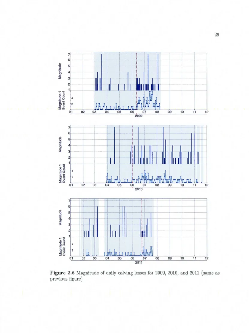
Figures 2.5, 2.6, and 2. 7 present the temporal distribution of all events over the

entire study period. Events of magnitude 5, 6, and 7, here considered to be major

events, occur between 3 and 9 times per year with inter-event intervals ranging

from a few days to as long as 2 months for an average of 38 days. Smaller events

experience significantly shorter repeat intervals, with multiple events occasionally

occurring on the same day. Events of magnitude 1, 2, and to some extent, 3, all

experience a marked increase in frequency in June immediately after the day of

and 2008), the frequency of small events decreases in August-September. Data

covering the end of the summer period are not available for 2009 and 2011, and

2010 presents generally low calving activity and a slowdown is not observable.

Major events appear to lack such seasonality, suggesting that they are driven

by different processes. Interannual variability in event size distribution is not

available for all months due to uneven coverage provided by the dataset. However,

some comparison is possible for 6 months, between April and September. Both

2010 and 2011 appear to exhibit subdued calving activity when it cornes to small

(magnitude 1 and 2) events. This can at least partly be explained by the change of

camera position which ended up hiding most activity occurring at the first 200-250

m of the front from 2010 onwards. In the first three years, rv303 of the observed

magnitude 1 events occurred within the first 250 m. This number drops to ,..,._,73 for the last two years. This observational bias creates no significant diff rence in

the occurrence of larger events of magnitude 2 and higher. 2.5.5 Calving styles and calving front geometry

Most days experience one or occasionally two events, not considering the isolated blocks detaching from the front (i.e. magnitude 1 events). One major drawback of the method used is that the sampling rate does not allow to determine whether

the mass lost in the 24 h period between images is the result of one major event

or of multiple smaller ones. It would therefore be useful to increase the sampling

rate and acquire for example hourly photographs during periods of high calving

activity. This explains in part the negative r lationship between major events and

smaller ones, which is the fact that fewer small events are detected on days where

larger sections of the front collapse, because the large events wipe the little ones

from the record. Major events affect the full thickness of the terminus, extend over several kilometres ( up to 4 km) across the front and produce an ice margin with a regular, linear or arcuate, geometry. Small events on the other hand cause the ice cliffs to become irregular and punctuated by small embayments.

r --6 ~ 5 .2 "§, 4

"'

:2 3 ~ë Q) ::> " 0 _::>(.) .".t:::_ t: t: Cl Q) "'> :2w 2 1 01 02 03 - - --·-·-1-·- - -+

~11111111

111

1~

1Jl1111

l11111111l

l

1 1 1 1 1

~N

r 04 05 06 07 08 2007 7F ---~ --- -, ~,j 6~ 1 ;- r· : Q) -0 .2 -E Cl

"'

:2 ~ë Q) ::> "0 ::>(.) ·ëë Cl Q) "'> :2w 5. 4 3, ~ 1

i

-~--=

01 02 03

ll

L

Jl

_jl

1111

1

1 1

li~

l111lul

li

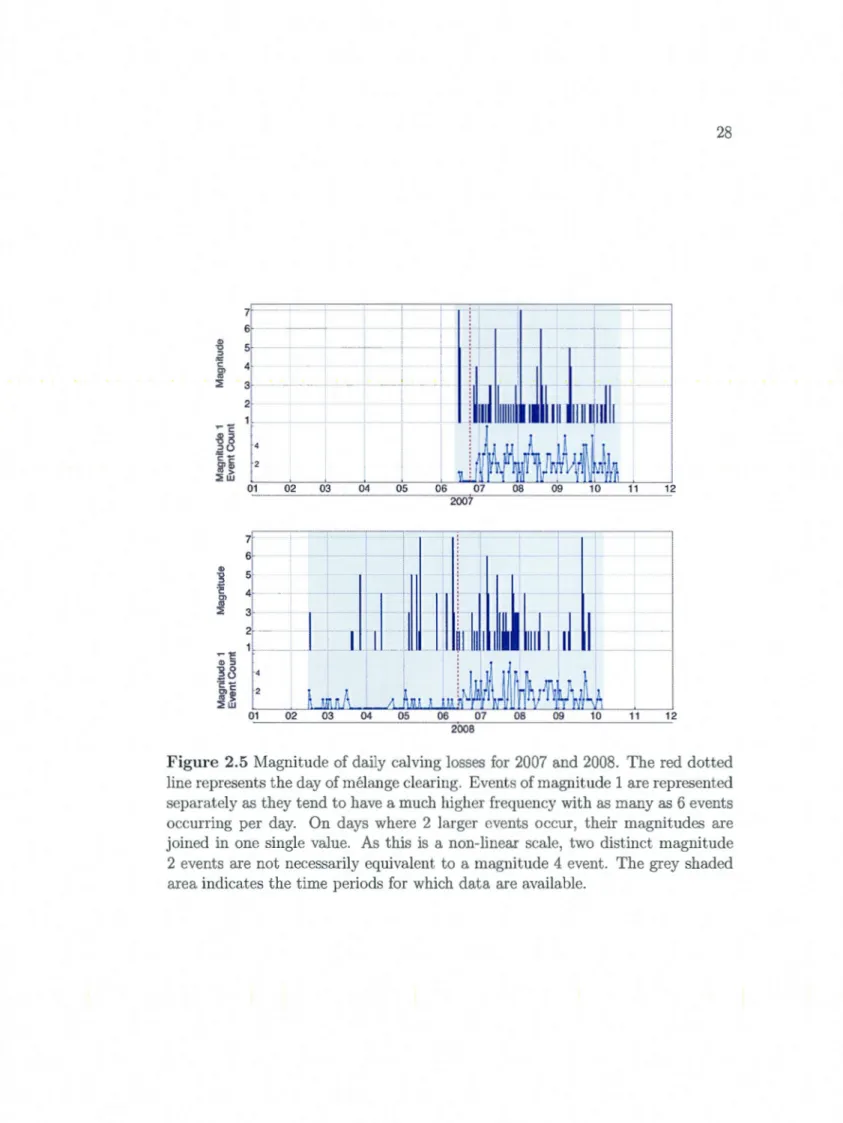
2008 11 12 11 12

Figure 2.5 Magnitude of daily calving lasses for 2007 and 2008. The red dotted line represents the day of mélange clearing. Events of magnitude 1 are represented separately as they tend to have a much higher frequency with as many as 6 events occurring per day. On days where 2 larger events occur, their magnitudes are joined in one single value. As this is a non-linear scale, two distinct magnitude 2 events are not necessarily equivalent to a magnitude 4 event. The grey shaded area indicates the time periods for which data are available.

7 6 ~ 5 _:J 'Ë 4 Ol

"'

:2 3 ~c: Q) :J "O 0 .ao "ëë Ol Q) "'> :2w 2 1 -+ - ~- 1 - .. i - -+- -·---~---·l 1

Jll

··

uh

1 -01 02 03 04 05 06 07 08 09 10 11 12 2009 7 1 i 6L '

,

--

-+---

'

- -

t

gi i i 1 : :2 3~ + • i- r 1 : ~c: Q) :J "O 0 .ao "ë ... Ol c " ' Q) :2 Ji Q) "O .a ï:: Ol

"'

:2

-~c Q) :J "O 0 .ao "ëë Ol Q) "'> :2w 1 . 1 :

2

r

•

1 1 ~ i ;. . 1ll1l 11

li

l I

1111

I

J

1111111 111111 06 07 08 09 10 11 12 2010 1-11--+-~ ----, --··----+---·---4 ~ 3 2 1

1~

11

I

-l

1111

I

~

h

1

I

! . 1 ' 1. , . ~.LI ; :_ ~~~!l.L~.__LlW~J1llJJ.J.ll..AL. 01 02 03 04 05 06 07 08 09 10 11 12 2011

Figure 2.6 Magnitude of daily calving losses for 2009, 2010, and 2011 (same as

1 -7 ' ' ' ' 1 '·

:

.

L

n

1

f

1 1

·

i

11

1

!

1

--i

l

l--1 --+ 6

---~

fü

I

I

.

~-~-~~--l~~

---·

..

:

;

,

-·-- -j---+- i

-'

i

.

1 Q) ' "'O 5 :::! _:!::::: c O'l m ₂ ,.... ë QJ :::i 'C 0

t

:

2 () · c ... 0) c: CO QJ :2 JJ

-2 (J) ü )> ~ 0 -l

1

--10 0 (j) -2 1 0 (j)

-01 04 07 1 0 0 1 0 4 07 1 0 01 0 4 0 7 10 01 04 0 7 10 0 1 0 4 07 10 0 1 2007 2008 2009 2010 • s A T ••• SST i n ner fjord -SST o u ter fjord Fig u re 2. 7 T o p : Ma g ni t ud e o f da il y ca l v in g lo sses fo r a ll years . B ot tom: Mo n t hl y mea n S AT s ( purpl e a r ea) a nd SST s for t h e inn e r ( d as h e d lin e) a nd o u te r (so lid lin e) f jord l ocat i o n s . Th e s h a d ed blu e a r ea r e pr ese n ts th e dur at i o n o f t he m e l t seaso n as d e ri ve d fr o m PDD s . Th e ve rti ca l r e d d as h e d lin es indi cate t h e i ce m é l a n ge cl ear in g day o b se r ve d on th e t im e l a p se im ages.

70, •

6ol

!

f :

so

l

:

4ol :

30

l

l

! :

20

;

;

10~ : Magnitude 2 t : 0_{5 .1-4l-}3 .. _{'""~""'2 ~~} 6_ Magnlt~de 5

d

lf

vm

: : : 1 o~~~~~~~~._, 5 4 3 2 Locat;on (km) 200 180~ 160~ 1401· t20·· 1001

so

f

60l 40( : Magnitude 1 1. 20' : : : ! Û"' Lt,L...t..-1..1 ... -.1~--.l-4...- . ..LJ 5 4 3 2 1 11 ~--·~··-···-~9.flÎ.llJ,ô2..?_.,--····-·1 10f : : : : 9r ! : ! ! a~ : : : 71 :..

.

'

.

• •

.

l • ' • • 6> • ' ' ' 5l 1 : : : • : : 4t : : 31 • • 2[ : ,t: ' ' . oL:..._..~: .. "-:"·--" .~:i.... .. , 5 4 3 2 1 Location (km)

Figure 2.8 Spatial distribution of all logged calving events across the 4.5 km

-wide front divided into 18 sections of 250 m each. Notice the different scale for

the vertical axis showing event count. The north sicle of the fjord is on the left.

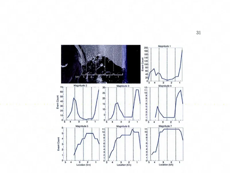
The spatial variability of calving across the front was analysed by dividing the front

into 18 sections of approximately 250 m each and documenting the location of each

event (Figure 2.8). Magnitude 1-4 events exhibit a strong bimodal distribution

with two peaks, one located at kilometre 1, and the other at the limit between

kilometre 3 and 4. The significantly stronger peak on the southern sicle of the

fjord likely represents a bias introduced by the perspective of the images and the

difficulties in identifying events further away from the camera. Major events of

magnitudes 5-7 on the other hand affect larger portions of the front and often

extend over multiple kilometres (up to 4 km) across the front. Their distribution

is therefore wider, with a shift towards the southern sicle of the fjord. Landsat

imagery (Figure 2.9) shows that they clearly align with the least crevassed sector

highest ice velocities (Chauché et al., 2014). As the major events appear to be

responsible for most of the mass loss through calving, the central sector of the front

experiences significantly higher losses than the margins. The spatial distribution

of low magnitude calving events on the other band coïncides with areas doser to

the margins, with closely spaced crevasses which experience a higher frequency of

events.

Figure 2.9 Landsat image (20 June 2014) showing the pattern of surface

crevasses. The white rectangles indicate de two highly crevassed sectors of the

terminus.

Figure 2.10 Calving front geometry before (06 May 2009) and after (16 June

2009) mélange clearing. Embayments form in locations where calving picks up

rapidly following mélange breakup.

The rapid increase in calving rates occurring at the time of ice mélange clearing

mainly concerns the low magnitude events and affects the more crevassed areas of the front. On four of the five years, large embayments are observed to form

rapidly over a few weeks in June as the mélange disintegrates. The mélange first loses its integrity near the lateral margins and calving rapidly picks up at these locations resulting in retreat. At the same time, the middle section of the front

continues to advance forming a large headland which extends as far as '""1 km further out into the fjord (Figure 2.10). The advance of the headland is rather short-lived and it quickly disintegrates in a series of larg r events returning the front to a more linear geometry in a matter of w eks.

Figure 2.11 Typical locations of glacial meltwater upwellings.

The spatial distribution of small events additionally seems to correlate with the spatial pattern of upwellings of glacial meltwater. Upwellings are observed on the timelapse imagery between June and September as well-defined plumes pushing

brash ice away from the ice cliffs (Figure 2.11). Localised meltwater discharge at the front has been observed to increase submarine melt rates which leads to undercutting of the ice cliffs and modifies the force balance at the front by

re-moving supporting ice (Motyka et al., 2003; O'Leary and Christoffersen, 2013; Chauché et al., 2014). Locations where meltwater emerges at the front are

there-fore expected to experience increased calving rates which creates a characteristic

front geometry punctuated by embayments. At Rink those embayments remain small and rather short-lived and the front remains relatively linear throughout the summer.

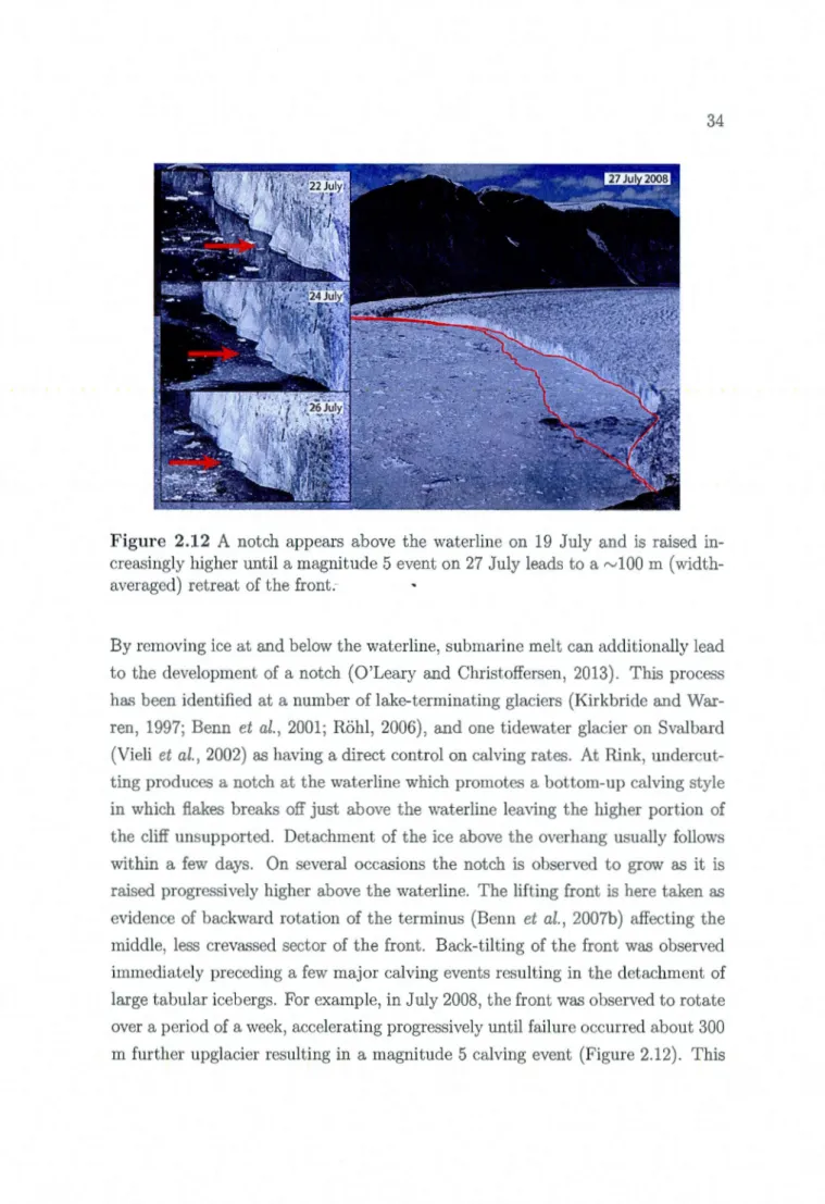
Figure 2.12 A notch appears above the waterline on 19 July and is raised

in-creasingly higher until a magnitude 5 event on 27 July leads to a rvlOO m (width -averaged) retreat of the front.

-By removing ice at and below the waterline, submarine melt can additionally lead to the development of a notch (O'Leary and Christoffersen, 2013). This process

has been identified at a number of lake-terminating glaciers (Kirkbride and Wa

r-ren, 1997; Benn et al., 2001; Rohl, 2006), and one tidewater glacier on Svalbard

(Vieli et al., 2002) as having a direct control on calving rates. At Rink, underc

ut-ting produces a notch at the waterline which promotes a bottom-up calving style

in which flakes breaks off just above the waterline leaving the higher portion of

the cliff unsupported. Detachment of the ice above the overhang usually follows

within a few days. On several occasions the notch is observed to grow as it is

raised progressively higher above the waterline. The lifting front is here taken as evidence of backward rotation of the terminus (Benn et al., 2007b) affecting the

middle, less crevassed sector of the front. Back-tilting of the front was observed

immediately preceding a few major calving events resulting in the detachment of large tabular icebergs. For example, in July 2008, the front was observed to rotate

over a period of a week, accelerating progressively until failure occurred about 300 m further upglacier resulting in a magnitude 5 calving event (Figure 2.12). This