Term structure of psychological interest rates: A behavioral test

HAL Id: halshs-00536910

https://halshs.archives-ouvertes.fr/halshs-00536910

HAL is a multi-disciplinary open access

archive for the deposit and dissemination of sci-entific research documents, whether they are pub-lished or not. The documents may come from teaching and research institutions in France or abroad, or from public or private research centers.

L’archive ouverte pluridisciplinaire HAL, est destinée au dépôt et à la diffusion de documents scientifiques de niveau recherche, publiés ou non, émanant des établissements d’enseignement et de recherche français ou étrangers, des laboratoires publics ou privés.

Term structure of psychological interest rates: A

behavioral test

Hubert de la Bruslerie

To cite this version:

Hubert de la Bruslerie. Term structure of psychological interest rates: A behavioral test. Southern Finance Association 2010 Conference, Nov 2010, Ashville, USA, États-Unis. �halshs-00536910�

1

Term structure of psychological interest rates: A behavioral test

Hubert de La Bruslerie Professor of Finance*

Abstract

A lot of empirical and behavioral studies underline the idea of a non-flat term structure of subjective interest rates with a decreasing slope. Using an empirical test, this paper aims at identifying in individual behaviors whether agents see their psychological value of time decreasing or not. We show that the subjective interest rate follows a negatively sloped term structure. It can be parameterized using two variables, one specifying the instantaneous time preference, the other characterizing the slope of the term structure. A trade-off law called “balancing pressure law” is identified between these two parameters. We show that the term structure of psychological rates depends strongly on gender, but appears not to be linked with life expectancy. We also question the cross relationship between risk aversion and time preference. From a theoretical point of view, these two variables stand as two different and independent dimensions of choice. However, empirically, both time preference attitude and slope seem directly influenced by risk attitude.

Keywords: hyperbolic discounting, time preference, behavioral economics, psychological time value, risk aversion

10/09/10

JEL classification: C9, D03, D91

*

University Paris Dauphine, DRM-Finance, Place du Mal de Lattre 75116 Paris France, mail: hlb@dauphine.fr. I want to thank Florent Pratlong, University Paris I Sorbonne, for his help in designing the questionnaire. This paper benefited from comments of Franck Moreau, University of Rennes I, Yi-Kai Su, University of Taiwan. It was presented at the HEC Geneva seminar of Finance, at the 7th AFFI International Finance Meeting in Paris, at the 2010 EFMA Annual Conference in Aarhus.

2

Introduction

If risk aversion is an important feature of economic and financial behaviors, the attitude of an agent with regard to time is also fundamental. The subjective value given to time, also known as the subjective interest rate or the subjective value of time, is identified as a core concept of the microeconomic literature. It is a fundamental parameter, which enters into economic or financial choices. We know that choices are comparisons between pleasures and pains (Bentham, Introduction to the Principles of Morals and Legislation, 1789), which are estimated at different times, now and in the future. The weighting factor of choices that makes preferences is subjective utility. The time dimension is rooted in the economic process of choice because different periods are considered. It is for this reason that we need to consider not only a subjective interest rate to discount future utility, but several subjective interest rates allowing the definition of a subjective or psychological discount function. There is a difference between the subjective interest rate, which is a variable used by an agent to discount his future utility, and the time preference hypothesis. The time preference hypothesis refers to the idea that an agent has a “preference for immediate utility compared with a future

utility” (Frederick et al., 2002, p. 351). We assume here that the economically rational agent

has a positive subjective interest rate. He discounts future utility.1 As a consequence, the time preference hypothesis implies that the rational agent (i) needs to subjectively evaluate time, (ii) discounts future utility and (iii) develops a set of multitemporal choices. Moreover, the subjective interest rate is often submitted to an additional hypothesis: it is assumed to be constant whatever the age of the individual or the time horizon considered in the choice. This is the standard micro-economic setting of individual choices. Combined with the hypothesis of time invariance of preferences (involving time separable utility function), it leads to the classical model of maximization of the sum of discounted future utilities, as introduced by Samuelson (1937). Individual decisions using a unique and constant subjective interest rate will refer to an exponential discounting function. In equilibrium models of consumption-investment, choices are specified with regard to a representative agent, which allows the consideration of available aggregated variables.

1

3 The hypothesis of a unique and constant subjective interest rate is very useful for further modeling and empirical tests. Using market equilibrium variables or the aggregate values of investment of a representative agent is easy. However, it involves a very poor view of intertemporal choice setting by individuals. Many empirical and behavioral studies underline the idea of a non-flat term structure of subjective interest rates with a decreasing slope. This hypothesis has to be crossed with individual behaviors.

This paper aims at identifying whether agents see their psychological value of time as decreasing or not. We questioned a sample of 243 individuals in order to analyze their attitude with regard to time. They were asked to give to time different psychological values at different points in the future. The difficulty here is staying at the psychological value level and not questioning a monetary value of time. Public interest rates are social prices of time in a market and they appear as alternative saving or investment goods. Here, we want to question not the utility of saving goods or financial assets, but the intertemporal comparison of personal utilities (wherever they come from). The psychological value of time derives from the individual perception of choices between the current “self” of the individual at time t and his future “selves” at times t+1, t+2…We show that the subjective interest rates are specific to each individual. They have a decreasing form coherent with a negatively sloped term structure. They can be parameterized using two individual parameters, one specifying the immediate term preference, the other characterizing the slope. A trade-off law is documented between the two parameters, which appear to follow a log-log relationship common to any individuals. The term structure of psychological interest rates does not appear linked with life expectancy, but strongly depends on gender. Individual subjective time preference does not show a tempus fugit effect.

Individual preferences are conditioned by few variables. A cross relationship between risk aversion and time preference is often questioned, at least on theoretical grounds. These two concepts stand as two different and independent dimensions. Empirically, time preference attitude and slope seem directly influenced by attitude with regard to risk.

The following paper is divided into 5 Sections. The first presents a review of the literature. Section 2 introduces the concept of free time and the questionnaire. Section 3 gives the results and tests some assumptions. Section 4 estimates the term structure of subjective

4 interest rates. The determinant variables explaining the subjective interest rates are analyzed in Section 5.

1-The literature

Fisher (1930) introduced the concept of rate of impatience in microeconomics choices. Samuelson (1937) developed a normative model of intertemporal choice using the discounted value of expected future utility. The idea is that an individual maximizes a set of utilities at different current and future periods. Referring to a “time separation” hypothesis, each periodic and specific future utility can be discounted. Individual choice will result from the combination of the utility dimension (which is itself influenced by the attitude toward risk) and the time dimension. The individual psychological price of time, also referred to as the rate of impatience, is an economic variable per se needed to build economic choices. Discounting the consequences of future decisions is at the heart of individual behaviors according to the standard micro-economic theory. The agent considers globally current and future expected utility, the latter being forecasted using available information. Samuelson introduces an identical subjective rate of interest, which results in a simple exponential discounting function in the standard microeconomic model.

( )

∑

δ

δ: annual constant psychological discount factor Ct: consumption at period t

U(Ct): consumption utility

Time is an economically valuable dimension. Von Mises (1949) recognizes the time preference hypothesis.2 He consequently mentions that individuals give a psychological value to time and their impatience rate should not be assimilated with the interest rates in the financial markets. Interest rates are the social price of time and are used to compare alternative consumption and investment opportunities. The psychological interest rate is used to discount subjective evaluation by individuals in their calculus, what he calls “economization”. For Von Mises, “The economization of time is independent of the

2

5

economization of economic goods and services. Even in the land of Cockaigne man would be forced to economize time, provided he were not immortal and not endowed with eternal youth and indestructible health and vigor. Although all his appetites could be satisfied immediately without any expenditure of labor, he would have to arrange his time schedule, as there are states of satisfaction which are incompatible and cannot be consummated at the same time.

For this man, too, time would be scarce and subject to the aspect of sooner and later”. 3 The

analysis of the variables which may explain individual time preference is very rich: remaining duration of life, health, youth will affect the level of the subjective interest rates. This approach opens the way to subjective interest rates, which are variable through time for the same individual according to his expected duration of life or his health. This is the first mention of a possible terms structure in the psychological value of time. A major theoretical question is set. Does intertemporal attitude depend on visceral features and is constant or, as suggested by Von Mises, does it depend on contingent variables?

Later and independently, this theoretical hypothesis was reinforced by empirical research questioning the exponential discount function. Empirical tests were developed to see whether individual subjective interest rates are constant whatever the time horizon of the choice. These tests generally invalidate the idea of flat impatience rates and lead to the conclusion of a decreasing term structure. Thaler (1981) was among the first to sustain that hypothesis by questioning individuals: “Which amount in respectively 1 month, 1 year or 10 years would you judge equivalent to 15 dollars now?” The median answers were $20 in 1 month, $50 in 1 year, and $100 in 10 years’ time. Thaler deduced a decreasing term structure of impatience rate with values of 345% for the one month horizon, 220% for the one year and 15% for the 10 years.

Experimental tests of the psychological discount function have been made on human individuals or animals by psychologists or psychiatrists. Chung and Herrnstein (1961) draw the conclusion that a decreasing hyperbola fits well the time preference function of animals. Considering human individuals, Ainslie (1992) and Loewenstein and Prelec (1992) model discount functions such as the hyperbolic curve δ(t)=(1+α.t)-γ/t, with t being the time horizon. This curve gives decreasing equivalent annual interest rates. The immediate subjective interest rate is equal to the parameter γ. Long-term psychological rates converge toward zero.

3

6 The decreasing term structure, as suggested by a hyperbolic model, would entail overdiscounting the immediate future vis-à-vis the far distant future. On the other hand, a flat term structure would ceteris paribus result in overdiscounting the distant future. The characteristics of hyperbolic (or any decreasing) subjective term structure is that the long-term future accounts for relatively more in solving the dynamic choice problems than the short term future. At the extreme, a myopic individual, who considers only the current period and the one that follows, will need only a short-term discount rate for the next period and is not concerned by the time inconsistency problem for onward periods (Loewenstein et Prelec, 1992). Laibson (1996) suggests the use of a “quasi-hyperbolic” discount function, which refers to two parameters: the standard discount coefficient δ and a second parameter β <1. At period t=1, the discount coefficient is β.δ. The following coefficients are multiplied by the unique β coefficients. This results in a discrete discount function {1, β.δ, βδ2, β.δ3…}. He was one of the first to mention that economic agents are more impatient when they undertake short-term arbitrage than when they make economic choices within a long-term horizon.

The theoretical problem with a non-flat term structure of psychological interest rates is their time inconsistency. The sequences of economic choices are ex ante incoherent, which is not rational in the homo economicus setting. The optimal choices that are calculated for period t using a discount factor δ(t) are not the same as those that will be preferred one period later using a factor δ(t-1) and discounted. Strotz (1956) underlined that ex ante the two sequences of consumption plans are dynamically incoherent. Time consistent setting of present and future consumptions using the available information implies that individuals cannot be irrational. Therefore the (only) simple solution is that psychological interest rates should be constant. However, in a situation of dynamic time inconsistent plans, intertemporal choices can also be analyzed as a conflict between different economically calculating agents, existing in the same individual. As Laibson (1996) points out, the “self” who decides at time t, enters into a strategic game with the optimizing “self” at time t+1. The multiple “selves” model is a way to cope with the “time inconsistency” consequence involved in non-flat psychological interest rates. Multiple “selves” is a psychological concept that allows the characterization of the peculiar nature of intertemporal choices (Frederick et al., 2002). On the other hand, time inconsistency may also derive from evolving preference functions such as “changing taste” preferences (Kahneman and Tversky, 1979; Tversky and Kahneman, 1992).

7 Thaler and Shefrin (1981) introduced the concept of multiple selves in a non-formalized way, which did not lead to a testable hypothesis. They analyzed the consistency of temporal choices in a theory of “self-control”. The agent has two “selves” in a conflict. The same individual is assumed to be at the same time a “planner” who organizes his consumption-investment choices looking at the long term and a myopic agent making choices on the very short-term horizon (a “doer”). The “doer” optimizes looking only at the next period. A conflict arises between the two different series of preferences. Thaler and Shefrin (1981) draw an analogy with agency conflict between manager and shareholders in a firm. The agent’s “self control” is a way to reduce the conflict between the planner’s self and the doer’s self. The only way for the planner to modify the myopic doer’s behavior is to control his behavior. This can be done either by modifying his preferences, or by imposing constraints or commitment rules to curb his choices. The devices to curb the behavior are classically incentives or rules. For instance, looking at the trade-off between consumption and investment, incentives may influence the behavior of the myopic agent by giving a strong moral and ethical value to saving. Self-limitation rules may be set to limit consumption and favor abstinence (equivalent to appetite suppressants for people who want to follow a diet regime).

Kahneman (1994) introduces a distinction between “decision utility”, which results from choices consciously made by an individual, more precisely the consequences of his choices, and “experienced utility”. Experienced utility stands at the global level of an individual’s well being. The difference between the two refers to “basic” needs and the psychological concerns of human beings (Frederick et al., 2002). In a behavioral approach, there are indirect utility elements that are exogenously given, received or inherited from the context of the individual, or they may also be an indirect consequence of his choices. These elements will depend on the context of the individual, on previous choices, on pure random externalities and on tensions between the different “selves” that make a personality and a character. The individual context links past to future choices. In the economic dimension, the difference between “decision utility” and “experienced utility” is a difference in linkage with a decision made at time t; it suggests that the instantaneous utility function is not constant.

In a behavioral approach, “time separability” exists and means that the individual can identify the instantaneous utilities from which he can build his global utility: global utility is

8 “the temporal integral of some transformation of instant utility”.4 Temporal aggregation means that the individual can compare two instantaneous utilities at different time periods by evaluating which one has the most important hedonic value. We are still in a psychological economic rationale of preferences. Kahnenam and Riis (2005, p. 8) add that “time is the last

human resource of his life and find a way to use it at best is an important goal both for the individual involved in his being and at the level of social choices aiming at human well-being”. This leads to the idea of time preference or positive psychological time value. This

also entails questions on the upper limit with regard to aggregating future instantaneous utilities. The end of human life imposes a limit in the definition of his time personality. The successors of the agent (his children, global society…) are not his economic “selves”. His identity will in the end die and be replaced by other actors and other preferences. This does not imply that the agent is indifferent to what can happen after his death. He can derive utility in passing on wealth or economic goods. His successors (if any and ex ante identified) will have different personalities and preferences.

The idea of identity involves consciousness of the structure of one’s preference: Is the agent conscious of the stability/instability of his tastes? Am I the same now as I was yesterday? Will I be the same tomorrow? There is as much strength of differentiation and of continuity between the “selves” of the same individual within time as there are between different agents who are close to each other and living at the same time in the same social group. In analyzing economic behavior, discounting temporal preferences is as rational as socially aggregating individual preferences. According to Frederick (2006): “It may be just as

rational to discount one’s (self) future utility, as to discount the utility of another distinct individual, because the distinction between the stage of one’s life may be as deep as the

distinction between individuals”.5The theoretical questions raised by intertemeporal

discounting are numerous and are listed in Soman et al. (2005) or Rohde (2010) for an axiomatic point of view. Experimental studies have privileged individual choices and answers. In that sense, they convey more information than looking at aggregated market data. Feather and Shaw (1999) try to evaluate the leisure opportunity cost of beach sports. This cost is traditionally estimated to be a fraction of the wage rate. A problem arises for individuals who are not employed and have no observable wages. The demand for leisure will depend jointly on the pure time preference and on the wage rate. The time devoted to work is not a

4 _{Cf. Kahneman et al. (1997), p. 388.} 5

9 discretionary continuous variable that an agent may easily optimize. Feather and Shaw underline that the “value of time” is not only given by a trade-off with the wage rate; it also depends on other hedonic variables. An estimate of the “shadow price of leisure time” is proposed by Lew and Larson (2005) in their evaluation of the discretionary wage. This concept assumes that the agent stands at his equilibrium between work and leisure and can make a trade-off. The evaluation of the leisure consumption is stochastic and is empirically estimated with regard to the consumption of leisure on Californian beaches. The implicit prices of leisure time are very different. They are high for employed or over-employed individuals, and lower for retired, unemployed and students. Warner and Pleeter (2001) analyzed the choices made by 60,000 American army members who were offered the choice of either a life annuity or an immediate indemnity on leaving the army. The actuarial rate used to define the annual cash flow was 17.5%, at a time when the interest rate offered in the financial market was 7%. The annual cash flow choice appeared financially better than the immediate payment. The empirical study showed that half of officers and around 10% of soldiers and civil employees chose the annual installments. This result evidences a very strong individual preference for the present time. The estimates of the psychological interest rate of army members by Warner and Pleeter were between 24% and 42%.

Shapiro (2005) made an empirical study of American individuals who benefited from a free allocation of “food stamps”. These subsidies are granted monthly. It was shown that the caloric consumption of those receiving the food stamps decreased by between 10 and 15% during the month. This implies a strong short-term preference. Calibrating a time preference function of a logarithmic agent, Shapiro obtains a daily subjective time discount coefficient of 0.996. Under the hypothesis of an exponential discount function, this is equivalent to an annual discount coefficient of 0.23 on a one-year horizon, i.e. a subjective interest rate of 320% per year. This estimate is viewed as too strong, so Shapiro questions the exponential subjective impatience hypothesis and uses the Laibson (1996) quasi-hyperbolic function to calibrate the data. With an estimated β of 0.96, he concludes that a hyperbolic function is better suited to high interest rates on the short-term end of the time preference curve. Kurz et al. (1973), using a simple questionnaire, concludes that the annual subjective interest rate is within the 36% to 76% range. Thaler and Shefrin (1981) also asked a very simple question: “Which money bonus do you want now instead of a 100 dollars bonus in a one year’s time?”. They highlight the influence of conditioning variables such as age, income level and marital status. They insist on the relationship between age and maturity: young people have to learn

10 and internalize the technique of behavioral self-control. Social categories are also important in explaining the subjective interest rate. Thaler and Shefrin evoke a decreasing structure of subjective interest rates. In the long term, agents are relatively more patient: for instance, I prefer two apples within 101 days from now than one apple within 100 days. However, in a short-term view, the rate of impatience is different: I prefer one apple now than two apples tomorrow. Frederick et al. (2002) collected the estimates of subjective discount factors resulting from thirty experimental studies. They crossed these subjective values of time with the time horizon of choices ranging from the very short-term (10 dollars now versus X dollars tomorrow) to the very long-term (10 dollars now versus Y dollars in 10 years). The average discount factors (average subjective interest rate) showed an increasing (decreasing) structure with the time horizon term structure. Frederick et al. point out that questions based on money comparisons may be polluted with the idea of the interest rate, which is a social and marketable price of time and not a subjective time preference used by individuals to set their personal choices.

Many experiments and studies have tried to identify the conditioning variable explaining individual time preference attitudes. The influencing variables are:

- Attitude of smokers: smokers have a psychological price of time, which appear higher

as compared with non smokers (Baker et al., 2003, Kirby and Petry, 2004, Ohmura et

al., 2005).

- Alcohol dependency: alcoholics have a larger psychological price of time. Serious

alcoholics discount future gains to a greater extent than do former alcoholics (Petry, 2001, Bjork et al., 2004). The same is true for drug addicts (Bretteville-Jensen, 1999, Kirby and Petry, 2004).

- Wealth level: rich households present subject interest rates that are 3 to 5% lower than

households with low income (Lawrance, 1991).

- Age: Young people are moderately patient (i.e. they have a low psychological price of

time). Patience increases with age and senior people have a larger psychological price of time (i.e. a lower discount factor) (Green et al., 1994). Life expectancy appears to influence and attenuate the relationship with age.

- Cognitive ability: Frederick (2005) shows the influence of cognitive abilities. In his

test, he uses an index of “cognitive reflection” (CRT, “Cognitive Reflection Test”), which spans the difference of behavior between individuals who behave intuitively without taking the time for reflection and those who act taking the time to analyze and

11 evaluate choices. The CRT index was crossed with both the dimensions of time preference and risk aversion using a sample of 3,428 respondents. A positive relationship between the CRT index and patience was highlighted: people showing high cognitive reflection are also more patient. A link was identified with risk attitude: people with a high CRT index are more prone to risk.

- Gender is a fundamental characteristic in the psychological valuation of time. For

instance, Frederick (2005) shows that women have a lower CRT index (correlated with impatience and a higher time preference) than men.

- Risk aversion also seems to play a role. According to Frederick (2005), there is a

common factor behind time preference and risk aversion. This hypothesis is important because it would mean that the two dimensions of risk aversion and time preference may be linked in human choices.

2-The concept of free time and the questionnaire

One important issue when dealing with individual time preference is knowing whether questions and choices have to be set in monetary units or not. Using a money equivalent places the individual in a framework of consumption power and leads to an underestimation of the answer. People are systematically exposed to confusion with saving decisions and interest rates. Comparing amounts of money now and later in the future is a saving choice and that decision is polluted by the existing possibility of deferring power consumption using existing market interest rates. When the outcomes are monetary, a normative behavior is based on Irving Fisher’s assertion that rational decision makers will borrow or lend so that their marginal rate of substitution between present and future money will equal the market interest rate.” As Read (2004) points out, “discount rates that exceed the opportunity cost of capital represent irrational behavior”. The pure time preference is independent of the content of current and future choices between consumption and saving. We need to compare the utility of consuming a product now and the utility of consuming the same product in the future. Comparison of “moneyed choices” refers or suggests interest rates and introduces confusion between the psychological price of alternative utility choices and the social price of time. Cairns and Van der Poole (2000, 2002) first used questionnaires with questions comparing amounts of money. Later they privileged studies without any reference to money

12 and compared dealing with a disease now with the possibility of deferring its onset further into the future.

The psychological value of time is the discounted factor applied to choice involving the future. This element is crucial in the dimension of intertemporal comparison at different times. The valuation ratio of two (utility) choices does not have a value in itself; it has a value relative to individual choices. It is not a general and shared price; it is a subjective ratio that should not be expressed in monetary units. Time is an open window for present and future choices and, possibly, future utility. Deferring or accelerating these choices expresses the personal value given to time. The idea of “free time” is used to identify an extra opportunity opened up to individuals to make new choices now or in the future. It does not say anything about the content of these choices. When comparing two apples in the future and one apple now, comparison develops within the framework of the utility of a given choice, i.e. to eat an apple. This involves the specific utility of an apple for someone who is fond of apples or that of another individual who hates apples. The idea of marginal free time opens up the space for new choices and additional utility independently of the content of the choice and the utility of the decision made within this new deferred opportunity to act economically. This free time is a window through which to enter into new economical and behavioral choices. It is not per se a set of substantial choices. It may have no value; it is not automatically linked to the consumption of goods, additional time to work or salary. The unit is “one hour of free time”, not its value in euros. This “free hour” is given once in the time horizon and is compared with other amount of “free time” given once in the near or far future. To our knowledge this concept has not been used in the previous empirical literature. This approach is not exposed to the “changing taste” hypothesis which states that a comparison between utilities linked to the same good at different time can be explained by a possible evolution of the intrinsic utility of the good through time. This is the “Horse and the Rider” metaphor mentioned by Soman et al. (2005). Rational agents can forecast the evolution of their future utility function. However, a projection bias is identified by Loewenstein et al. (2003) who explain that the agents make their future tastes similar to their current tastes. The idea of “free time” disentangles time preference from the other factors that drive people to devalue future outcomes.

An additional hour of free time at period t is compared with an additional hour of free time later. The hypothesis of time preference means that an hour of free time now is more

13 valuable than one hour of free time later in the future. The relative ratio between the two gives an implicit price, which is the individual’s subjective interest rate.

The questionnaire

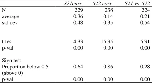
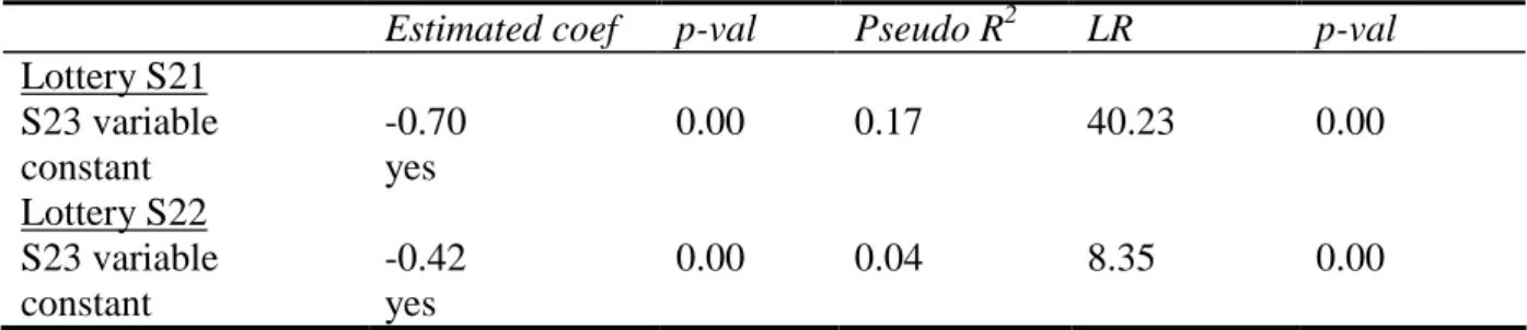
The questions and a preliminary form were firstly tested on marketing students of the master’s degree of the University Paris Sorbonne (Jolibert and Jourdan, 2006). These answers were not considered in the subsequent main test. The form itself is structured in four blocks of questions. The questionnaire was anonymously submitted to individuals. The first block of questions (block S) are questions about the characteristics of the respondent. Characteristics are unambiguous: date of birth, gender, place of birth, native language…(see Annex 1) Questions related to attitude and behavior cover the perception of time, the importance of passing on something to one’s children; three questions are devoted to attitudes regarding risk and risk aversion (S21, S22, S23). Two questions propose a traditional choice between playing an uncertain lottery and a certain income. Personal attitude vis-à-vis the risk is questioned on a scale between risk-lovers and absolute risk averters.

The block A questions introduce the idea of “free time”. What we want to analyze is the attitude vis-à-vis a pure space of time open to any economical or behavioral choice. When giving the form to respondents, we introduced the questionnaire by saying: “imagine that a day is now 25 hours instead of 24, what is the importance of that extra new hour for you?”. We want to identify individual preference for an extra space of choices before these choices are effectively made. In that sense, we do not need to rely on rational assumptions linked to choices. Respondents are faced with choices and the valuation of their utility. We want to compare the preferences of this extra window of space for new choices between, for instance, now and X years in the future. Respondents were asked to compare a period of free time now and a period of free time at a given time in the future. We recognize that this setting makes two implicit behavioral assumptions: (i) the additional value of one awarded “free hour” is symmetric to the value of one free hour subtracted from the daily time horizon (“imagine that a day is now 23 hours instead of 24…”); (ii) the imagination of each one has to fill this new extra space of time. The way each one may fill this new pure time depends on the context of an economic choice led by scarcity of time (Von Mises, 1949). The way someone imagine leisure for instance is not the same if he is retired or if we focus to active people facing a

14 leisure/work choice. Busy executives may systematically view “free time“ as leisure. Here, fortunately our sample is composed of students and retired people and not of executives.

A1.-Would you prefer 1 extra hour of free time now or 2 hours of free time in 1 year’s time?

A2. -Would you prefer 1 extra hour of free time now or 5 hours of free time in 5 years’ time?

A3. -Would you prefer 1 extra hour of free time in 1 year’s time or 5 hours of free time in 6 years’ time?

A4. -Would you prefer 2 extra hours of free time in 10 years’ time or a set of 1 hour of free time now and 1 hour of free time in 20 years’ time?

A5. -Would you prefer 4 extra hours of free time in 10 years’ time or a set of 1 hour of free time now and 1 hour of free time in 20 years’ time?

A6. -Would you prefer 2 extra hours of free time in 5 years’ time or a set of 1 hour of free time now and 1 hour of free time in 20 years’ time?

A7. -Would you prefer a set of 1 extra hour of free time now and 1 hour of free time in 20 years’ time or 2 hours of free time in 10 years’ time?

A8 -Would you prefer to have in 10 years’ time 2 hours of extra free time for yourself or to get in 10 years’ time a set of one hour of free time for yourself and 1 hour of free time for one of your relatives?

Table 1 – Block A questions

(Answers with 3 alternative choices: first alternative, second alternative and indifference between the two choices. Indifferent choices would not be considered in the analysis)

Block B is a series of six questions on the relative value of one hour of free time in the future compared with one hour of free time now. Nine ordinal choices are proposed linked with a range of values expressed in number of hours. For instance, item 3 refers to a range of [2 to 6] hours. Respondents were asked to compare one hour of free time now and X hours in the future. By checking item 3, the respondent is showing that he considers one hour of free time now to be equivalent to 2 to 6 hours in the future. Different time horizons are questioned: 1 year ahead, 5 years, 10 years, 20 years, 30 years and 50 years corresponding respectively to questions B1 to B6. Questions B7 and B8 deal with curvature comparing a package of 15 hours of free time at two time horizons and 15 hours awarded at a medium term horizon.

15 Questions B1-B6 are as follows: One extra hour of free time now is equivalent to how many hours of free time in 1 year’s time (respectively 5 years, 10 years, 20 years, 30 years and 50 years)? The answer should be one of the 9 ordered choices:

1- Less than 1h in 1year (respectively 5, 10, 20, 30, 50 years) 2- Between 1h and 2h in 1y (id)

3- Between 2h and 6h in 1y (id) 4- Between 6h and 12h in 1y (id) 5- Between 12h and 22h in 1y (id) 6- Between 22h and 36h in 1y (id) 7- Between 36h and 52h in 1y (id) 8- Between 52h and 78h in 1y (id) 9- More than 78h in 1y (id)

The same questions were submitted again after the respondent was asked to read a mortality table. In the block C questions, people had to compute their life expectancy taking into account their date of birth and their gender. Each respondent had to calculate the probable year of his death and his expected remaining duration of life from the present day. Then, after being informed of his true average life expectancy, questions identical to B1-B8 were asked again (questions C6-C13).

The block C questions will be used to cope with the problem of perception of time. The respondent may answer according not to the objective duration of time but his own perception of time. Zauberman et al. (2009) claim that seemingly impatient choices and hyperbolic individual discounting, may be explained by the subjective perception of time. A discrepancy appears in empirical test and the subjective sensitivity to an objective variation in time is low. The Weber-Fechner law states that the relationship between the objective time change and its subjective perception follows a logarithmic function. This one contracts the objective time stimulus (Zauberman et al., 2009).

Data

The sample was put together from answers from 243 individuals. Two different categories of people were questioned using the questionnaire form. Most of the respondents were students from the Paris Sorbonne University. They are following management and

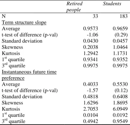
16 business economics studies and are in the graduation year of their bachelor’s or master’s degree. A sub sample of retired people aged 58 or more were interviewed in the French city of Reims (26 people) and by sending the questionnaires by mail to retired men and women in rural areas of France (32 respondents).6 They were members of a non-profit organization for retired people.7 Their average age was 67.1 years. The student sub-sample (185 people) was on average 22.1 years old. The two sub-samples are very distinct since we did not have any respondents born in the 1958-1976 period.

The questionnaire was answered during the academic year 2007-2008. The global average age of the whole sample was 32.8 years. Of the total sample, 58% were women. Only 56 respondents (23%) had children (average number of children was 2.03); 47 were grandparents. 88 of the respondents (36.5%) had thought about passing on something to their children. Of the others, 106 (44%) said they would think about it. However, a minority of 19% claimed that they were not motivated by passing on anything to their children. Globally, 49% of the individuals considered that they had something valuable (i.e. capital or knowledge) to pass on to their children.

average standard dev min max N

Date of birth 1974.18 19.64 1920 1988 243

Gender (0:men/1 women) 0.59 0.49 0 1 243

Number of children 2.03 1.06 0 5 56

Ability to speak another foreign language fluently (0:yes/1:no)

0.55 0.49 0 1 240

Currently a smoker (0:yes/1:no) 0.85 0.35 0 1 240

Education level 4.16 1.14 1 6 242

Monthly financial expenses category (1 to 6)

2.29 1.42 1 6 240

Perception of the importance of free time (ordered from 1, no to 6, of the utmost importance)

4.12 1.22 1 6 241

Financial planning horizon (1 to 4)

1.73 0.88 1 4 243

Planning to pass on capital and knowledge to children or other relatives (0:yes/1:no)

0.63 0.48 0 1 241

Importance of passing on capital and knowledge (from 1

2.60 1.21 1 6 242

6 _{A total of 250 questionnaires were distributed by the Fédération des Ainés Ruraux to their members.}

7 _{I would like to thank for their support Mrs Renate Gossart, President of the association “Les panthères grises”}

located in Reims and Mrs Delphine Guillaume in charge of internal communication at the Fédération Nationale des Ainés Ruraux, www.ainesruraux.org.

17 to 6)

Perception of risk attitude 3.40 1.34 1 6 243 Table 2 – Descriptive statistics of the sample

(Education level: answers from 1 (autodidact) to 6 (master’s degree); Monthly financial expenses by ordered categories: 1: below 300€ up to 6: more than 2500€; Financial planning horizon ordered from 1 to 4: 1 in coming months, 4 over the next 10 years; Importance of passing on capital and knowledge: 1, null, to 6, huge; Risk attitude: ordinal value from 1, risk lover, to 6, absolute risk rejection.)

3-Results

3.1 Qualitative time preference

Questions A1 to A8 aim at testing qualitatively the time preference hypothesis by advancing two propositions. The respondent can state a preference for one or the other or can say that the two are equivalent. If the answer is indifference, it is withdrawn from the data. We only consider choices expressed as preferences. Question A1 tests the time preference hypothesis by asking the preference of individuals between 1 hour of free time now (0) and 2 hours of free time 1 year ahead (1). The average answer (indifference excluded) is 0.33. This is significantly above zero. The idea of a trade-off between the present and the future can be accepted if a price exists, i.e. a preference of 1 hour now vs. 2 hours tomorrow. The test of equality of the A1 answer compared to a random average answer of 0.5 is rejected. However, the t-test assumes a normal distribution. This assumption is weak. We also consider a sign test (proportion below 0.5=0.64, p-val:0.00). It confirms the previous one.

A2 is the same question with a trade-off further in the future (1 hour now vs. 5 hours in 5 years). The average answer is 0.34. This is significantly different and lower than a random 0.5 answer.

The A1 vs. A2 test allows the checking of a difference in pricing the future. The null shows that the two means are not different. A p-value above the usual significance levels does not reject the null. The difference is not significant (p-value of the t-test: 0.00). This test is reliable because the A1-A2 difference is normal (Jarque-Bera statistic=64.90; p:0.00). This means that 2 hours in 1 year’s time are equivalent (not different from) 5 hours in 5 years’ time. The sign test gives 82% of zero differences. The implicit discount factor (5/2=2.5) is 26% a year (for a 1-5y horizon).

18

A1 corr. A2 corr. A1 vs. A2 A3 corr. A2 vs.A3

N 209 217 209 191 187 average 0.33 0.34 0.00 0.45 0.08 std dev 0.47 0.47 0.42 0.55 0.41 t-test -5.39 -4.94 0.48 -1.38 2.65 p-val 0.00 0.00 0.63 0.17 0.01 Sign test Proportion below 0.5 0.67 0.66 0.82 0.55 0.82 p-val 0.00 0.00 0.00 0.07 0.00

Table 3 – Results of the block A questions (I)

(corr.: answers corrected to eliminate indifferent choices; only 0/1 answers are taken into account; question A1 is comparison of 1 extra hour of free time now or 2 hours of free time in 1 year’s time; question A2 is comparison of 1 extra hour of free time now or 5 hours of free time in 5 years’ time; question A3 is comparison of 1 extra hour of free time in 1 year’s time or 5 hours of free time in 6 years’ time; A1 vs. A2 is the difference of A1 and A2 dummy vectors (similar for A2 vs. A3)

Question A3 is the same as A2 but put forward by 1 year. The average answer is 0.45. The t-test and the sign test show that the answer is not different compared with a random answer of 0.50. It means there is indifference between the two terms of choices suggested in question A3. We compared the answers to A2 to check whether the results are the same. A3 is significantly different from A2. According to the t-test, the hypothesis of difference is accepted, but it is rejected looking at the sign test. These results are contradictory. The statistic A3 minus A2 is normally distributed (JB=60.16, p:0.00); we privileged the t-test. This means that when the choice is put forward by 1 year, the preference for the time closer to the present date decreases. If the time preference had been the same, i.e. if exponential discounting were true, delaying the same choice by 1 year should have given the same result in questions A2 and A3. Here, the trade-off price is not the same. That result suggests a non-flat subjective interest rate. A decreasing curb will make the short-term side of the trade-off less attractive and place a larger weight on the long-term proposition. It is for this reason that we get an average answer of 0.45 for question A2 and above 0.37 for question A3. However, the two sets of choices are still coherent. The Spearman correlation between A2 and A3 is significant and positive (+0.65, p-val:0.00).

19 Question A4 tests the curvature of the time preference function. It asks whether individuals prefer 2 hours of free time within 10 years or a package of 1 hour now and 1 hour within 20 years. If (naïve) linearity prevails, under a flat curve, the two terms are equivalent, so the answer should be the average of 0 and 1, i.e. 0.5. We get an average answer of 0.66. The t-test against 0.5 and the sign test confirm this result to be significantly above a 50% probability. By preferring the package, individuals may have a decreasing time curve preference, i.e. a decreasing subjective price of time.

Question A5 modifies the term of the curvature. It gives a greater weight to the medium term choice (doubling it to 4 hours against 2 hours in question A4). The terms of the package remain the same. The preference for the medium-term time horizon choice (choice 0) increases logically with an average answer of 0.34. Referring both to the t-test and the sign test, this is significantly lower than 0.5. Question A5 is not meaningful in analyzing curvature because the relative terms are not comparable and not linear in the time horizon. However, it confirms that individuals are time rational. The choice (0) in A5 is logically better than the one proposed in A4. Using linear approximation and the results from A4 and A5, it means that to get indifference between X hours in 10 years’ time and a package of 2 hours (one now and one in 20 years), we should give (0.66-0.5)x(4-2)/(0.66-0.34)=1.00 hour more. This means 3.00 hours in 10 years’ time compares with a set of 2 hours now and in 20 years’ time.

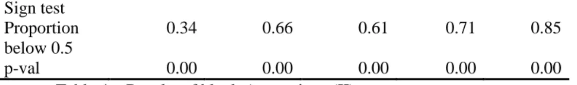
Question A6 is another way to test the curvature. The choice is similar to A5. The package is the same, but the medium term proposal is now 2 hours within 5 years (instead of 10 years in question A4). We expected that individuals with a preference for the present would choose the first answer compared with question A4. The average value is 0.39 compared with 0.66 in question A4. This is significantly below the random average answer of 0.50.

A4 corr. A5 corr. A6 corr. A4 vs. A6 A5 vs. A6

N 173 173 175 157 163

average 0.66 0.34 0.39 0.25 0.05

std dev 0.47 0.47 0.49 0.48 0.40

t-test 4.41 -4.59 -2.86 6.66 1.58

20 Sign test Proportion below 0.5 0.34 0.66 0.61 0.71 0.85 p-val 0.00 0.00 0.00 0.00 0.00

Table 4 – Results of block A questions (II)

(corr.: answers corrected to eliminate indifferent choices; only 0/1 answers are taken into account; question A4 is comparison of 2 extra hours of free time in 10 years’ time or a set of 1 hour of free time now and 1 hour of free time in 20 years’ time; question A5 is comparison of 4 extra hours of free time in 10 years’ time or a set of 1 hour of free time now and 1 hour of free time in 20 years’ time; question A6 is comparison of 2 extra hours of free time in 5 years’ time or a set of 1 hour of free time now and 1 hour of free time in 20 years’ time; A4 vs. A6 is the difference of A4 and A6 dummy vectors (similar for A5 vs. A6)

We will now consider the difference A4 vs. A6; it is normally distributed (JB=10.14, p:0.01). The difference between A6 and A4 is significant. The results are not the same as comparing A6 answers to those to the A5 question. When testing the hypothesis of different means between A6 and A5, we reject it. Using a sign test, we have a different conclusion with an average probability of an identical median of 85%. We will accept the conclusion of the t-test on the basis that data are normally distributed (JB=78.82, p:0.00) and that the sign t-test is less robust. This means that 4 hours in 10 years’ time are equivalent to 2 hours within 5 years. The psychological (annual) interest rate for the 5-10 year horizon that emerges is, therefore, 14.9%. This is lower than the 26% average subjective rate for the 1-5 year horizon.

We can mix the A4 and A6 results and use a linear approximation to find indifference between 2 hours in the future and the package (1h now + 1h in 20 years’ time). We have: (0.66-0.5) x (10-5)/(0.66-0.39) = 2.96 years. This means that 2 hours in 7.96 years’ time are equivalent to the package and the package is equivalent to 3.00 hours in 10 years’ time (see above). The variation between 7.96 and 10 years is 2.04 years for an increase of 1.00 hours of free time.

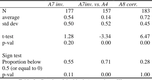
Question A7 is identical to A4 but presented in reverse order. The idea here is to test if respondents are coherent. The answers should be strictly opposite to those of A4. We inverted the A7 answers to get an average value of 0.54. This is not significantly different from 0.5 (in contrast with the A4 question). The test of the difference between A4 and inverted A7 shows a significant and unexpected difference according to the t-test. However, the t-test should be disregarded insofar as the A4 vs. inverted A7 variable is not normally distributed (Jarque-Bera=1.53, p:0.46). The sign test shows no significant difference. The Spearman rank

21 correlation coefficient between A4 and inverted A7 is 0.43. This is significantly positive (p=0.00). Hopefully, the same respondents are giving the same answer to similar questions in the questionnaire.

Question A8 is a test of altruism. After correction for indifference, the average value is 0.72, closer to 1 (altruistic attitude) than to 0 (personal individualism). The test vs. a random 0.5 value is significant. The Spearman coefficient was calculated to cross with curvature (question A4). The coefficient is 0.01. This is non significant (p=0.30). Altruism does not seem to be linked with curvature, i.e. temporality in the subjective price of time. These are two separate dimensions of human behavior.

A7 inv. A7inv. vs. A4 A8 corr.

N 177 157 183 average 0.54 0.14 0.72 std dev 0.50 0.52 0.45 t-test 1.28 -3.34 6.47 p-val 0.20 0.00 0.00 Sign test Proportion below 0.5 (or equal to 0) 0.55 0.71 0.28 p-val 0.11 0.00 1.00

Table 5 – Results of the block A questions (III)

(inv.: answers are corrected to eliminate indifferent answers and are inverted; corr.: corrected to eliminate indifferent choices; only 0/1 answers are taken into account; question A4 is comparison of 2 extra hours of free time in 10 years’ time or a set of 1 hour of free time now and 1 hour of free time in 20 years’ time; question A5 is comparison of a set of 1 extra hour of free time now and 1 hour of free time in 20 years’ time or 2 hours of free time in 10 years’ time; question 8 is, in 10 years’ time, comparison of 2 hours of extra free time for yourself or to get in 10 years’ time a set of one hour of free time for yourself and 1 hour of free time for one of your relatives)

3.2 Quantitative time preference evaluation

The direct price of time is tested through questions B1 to B6 considering the “price” of one hour of “free time” at different time horizons 1y, 5y, 10y, 20y, 30y and 50y. A measure of the subjective price of time is built considering the increase in the relative value of one hour of free time now and one hour later. If the subjective price of that hour increases, it

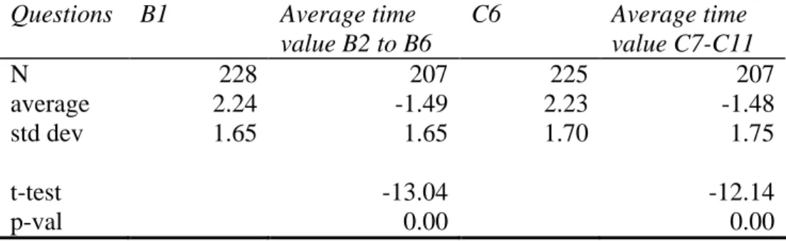
22 means that the time has a cost. We compared the individual answers to question B1 with the average answer to questions B2 to B6. If an individual answers, for instance, 2 to question B1, it means he gives a value of 1 to 2 h of free time in 1 year in the future compared with for one hour of free time now. If the average answer to the same question, but deferred forward in time (question B2), is 4, it means than the relative ratio of his personal time value is 6 to 9 hours compared to one hour now. We calculated the (possibly) negative slope of the subjective interest rate as the difference between the B1 answer and the average relative ratio resulting from questions B2 to B6. For instance, the previous respondent will yield a value of -2 (i.e. 2 at question B1 minus 4 at question B2); this shows a time preference attitude with deferred free time having less value than a near current free time opportunity. If the average difference is negative, this indicates globally a positive price for time (or a preference for immediacy). Looking at the answers, the average value of the subjective price for time indicator is effectively negative (-1.49) and significantly different from null. The answer is the same with the “informed” set of respondents. Questions C6 to C11 correspond exactly to questions B1-B6. The answer to question C6 was compared in the same way to the average answers considering a deferred horizon from 5 to 50 years (i.e. questions C7 to C11). The average value of the informed price of time indicator is significantly negative (-1.48).

Questions B1 Average time

value B2 to B6 C6 Average time value C7-C11 N 228 207 225 207 average 2.24 -1.49 2.23 -1.48 std dev 1.65 1.65 1.70 1.75 t-test -13.04 -12.14 p-val 0.00 0.00

Table 6 – Results of block B and C questions

(Each individual question is comparison of one extra hour of free time now and its equivalent number of hours of free time in respectively 1 year, 5 years, 10 years, 20 years, 30 years and 50 years’ period of time; answers are pre-coded within 9 ordered ranges; the set of questions B1-B6 is asked before delivering new information, the set of questions C6-C11 is asked after; the delivery of new information; new information is the expectancy life table of French population and the calculation by the respondent himself of his expected date of death; average time value is for each individual the difference between the average answer to question B2 to B6 and his answer to question B1, a negative figure means an increase of the value of time with a longer horizon; same for average answers to deferred horizon C7-C11 and question C6)

23 When informed of his true average life expectancy, the individual does not seem to modify his answer regarding his subjective price of time. The score decreases from 2.24 (question B1) to 2.23 (question C6). The difference between questions B1 and C6 is not significant (t-test=-0.15, p:0.88). The same is true for the subjective price of time before and after (t-test=-0.13, p:0.89). The two scores of subjective price of time show a strong correlation (Pearson correlation of +0.75, p:0.00). Salient and objective information given on time delay does not change the structure of the answers. We draw the conclusion that objective information on time does not modify its individual perception. Contrary to Zauberman et al. (2009) our result does not seem to be contaminated by a time perception effect. The decreasing slope of the individual term structure of psychological rates seems strong.

4-The term structure of subjective time preference

We calculated the average answer to the subjective price of time. Each question can be answered from checking ordinal values from 1 (a future free hour has a lower price than the current free time hour) up to 9 (i.e. one free time hour in the future has less value than 45 seconds today). Answer 1 is economically irrational in terms of time preference. It means a preference for the future compared to the present. It could also mean that the respondent did not understand the question.

The integer answers from 1 to 9 are trade-off relative values. The average ordinal answers to each question have been converted into subjective interest rates using the mid-range value. For instance, if a given individual answers 4 to question B2, he says that he will ask for between 6 and 12 hours of future free time 5 years ahead to be equivalent to one hour just now. Taking the mid-point of 9 hours in 5 years’ time, we derive an implicit subjective price of time of 55.18% per year.8

Taking the average value of the choices of the individuals, we obtain a collective time value preference. Table 7 shows the average answers with regard to the 6 time horizons. The structure of the average psychological interest rates clearly decreases with the time horizon. The short-term rate is 135.31% (1 year ahead); it decreases to 5.80% (50 years horizon). The

8

24 data collected after delivering objective information on life expectancy are similar. The term structure of psychological interest rates decreases from 117.53% to 5.97%.

Horizon (years) 1 5 10 20 30 50

Panel A Before information

Av. ordinal answer 2.3904 2.9248 3.4509 4.0045 4.3756 4.9074 Av. number of future hours for one

free time hour now

2.4759 3.8119 6.2545 9.0360 12.0045 16.2593

Implicit subjective interest rate 1.4759 0.3069 0.2012 0.1163 0.0864 0.0574 Panel B After information

Av. ordinal answer 2.4044 2.9381 3.4395 3.9452 4.3052 4.9761 Av. number of future hours for one

free time hour now

2.5111 3.8451 6.1973 8.7260 11.4413 16.8086

Implicit subjective interest rate 1.5111 0.3091 0.2001 0.1144 0.0846 0.0581 Table 7 – Estimate of average subjective interest rates

(Average ordinal: average of answers from 1 to 9 without corrections of outliers; Average number of future hours: number of future hours equivalent to one hour now calculated from the average answer by interpolating the mid-range of the ordinal answer (see Table A2 in Annex); implicit subjective rate: annual equivalent rate calculated using the maturity and the ratio of the number of future hours compared to one hour now; before information relates to block B questions; after information relates to block C questions; information delivered between the two is the statistical mortality table and the average life expectancy of the respondent) Before Information y = 0.5469e-0.0537x 0 0.2 0.4 0.6 0.8 1 1.2 1.4 1.6 0 10 20 30 40 50 60

25 Figure 1 – Average estimate of subjective interest rates (Before information)

(Source: Table 3; fitted using an exponential model)

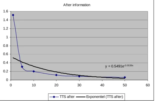
After information y = 0.5491e-0.0539x 0 0.2 0.4 0.6 0.8 1 1.2 1.4 1.6 0 10 20 30 40 50 60

TTS after Exponentiel (TTS after)

Figure 2 – Average estimate of subjective interest rates (After information) (Source: Table 3; fitted using an exponential model)

The fitted term structure of subjective interest rates is calculated using an exponential

model: t

a b t

r()= . .9 The estimation is performed on average data from Table 7. The b coefficient is the instantaneous subjective interest rate to future free time one second in the future. The fitted values are 55% (before and after information). The subjective price of time is characterized by a negative slope in the term structure curve. The log of the slope is a yearly -5.37% (before information) and -5.39% (after).

Looking at each individual, we transform his ordinal answer to annual implicit subjective rates using a correspondence table (see Annex). We corrected outliers particularly for wrong answers at question 1 about the relative ratio of one hour in one year. Wrong answers above 4 at question B1 (C6) will bias upward the implicit rates and result in abnormally high implicit rates. This may be due to a misunderstanding of the question. We decided not to remove these answers but to limit the maximum subjective rate to 500%. Descriptive statistics of the term structure of subjective interest rates of each respondent are given in Table 8.

9

26

Variable N average std. dev. Minimum Maximum

AV1 228 1.397184 1.713725 0.001000 5.000000 AV5 226 0.320404 0.339724 0.001000 1.390116 AV10 224 0.184333 0.167918 0.001000 0.546000 AV20 222 0.103912 0.084450 0.001000 0.243382 AV30 221 0.074331 0.057571 0.001000 0.156298 AV50 216 0.048872 0.035622 0.001000 0.091043 Table 8 - Descriptive statistics for individual subjective interest rates

(Time horizon 1y, 5y, 10y, 20y, 30y, 50y; source: relative price ratios from questions B1 to B6, converted into annual interest rates using the correspondence table A2 in Annex)

Looking at average values, the term structure seems clearly negative. It starts from an average 140% for the psychological interest rate for the 1 year horizon. This high figure is partly explained by possible errors in understanding the question and by outlier answers that have not been removed. At the end of the term structure, the rate is 4.9% for a 50 year horizon.

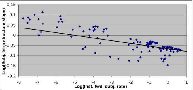
For each individual, we have a six point estimate of his psychological time preference structure. We fitted each individual term structure using an exponential two variable model. Each individual’s characteristic time preference structure can be defined using a couple of parameters, which are the intercept instantaneous interest rate and the slope. Over the whole sample, the average estimated parameter for the slope is 0.96 (which corresponds to a log of the slope of -3.60% yearly). The average estimates intercept of the exponential model is 0.53 (i.e. a 53% instantaneous forward interest rate). Results are similar when considering the answers to the C questions. 10

When we regress the individual bi estimates of the intercepts and the individual slopes ai, we obtain a -0.567 coefficient of correlation. Among individuals, if someone has a strong

immediate time preference, his long-term time trade-off is smoother with a lower negative slope with time horizon. This relationship is confirmed even if we add new information about the “true and average” life expectancy. This raw correlation indicates the existence of a relationship between the instantaneous forward subjective rate of the two parameters and the

10 _{These questions are answered after giving objective information to respondents regarding their life}

27 slope of the term structure of time value; however, it does not tell us anything about the form of the relationship. The linear form is not the best one. We also tested a log-log form. That gives a better fit with an R2 value of 0.573 (correlation of -0.76, see table 9).

β α

Estimated coefficient -0.01322 -0.0663

p-value 0.00 0.00

R2 0.5727

Table 9 – Log-log relationship between individual slope and intercept estimates of subjective term structure discount

(Relation is log(ai) = α +β log(bi) where ai.are term structure slope estimates; bi are

instantaneous forward rate estimates; t

a b t r()= . ; N=216) -0.2 -0.15 -0.1 -0.05 0 0.05 0.1 0.15 -8 -7 -6 -5 -4 -3 -2 -1 0 1

Log(Inst. fwd subj. rate)

L o g (S u b j. t e rm s tr u c tu re s lo p e )

Figure 3 – Log-log relationship between individual intercepts and slopes

We can draw the two following conclusions:

- The individual’s term structure of subjective psychological interest is decreasing. They are characterized by a couple of parameters corresponding to the instantaneous forward interest rate and the decreasing slope of his personal term structure of interest rate.

- A negative relationship exists between the two parameters defining the term structure of subjective rates: an individual with a strong short-term time preference experiences a more negative slope. He penalizes the deferred future relatively less compared with an individual whose instantaneous short-term interest rate is small.

28 As a result, a behavioral “law” may be formulated: those with a high immediate time preference have a relatively less demanding time preference in the deferred future. The original time preference hypothesis needs to be conceptualized at a deeper level: the strength of that preference does not result in an equal pressure directed toward the future. Time has a psychological price, but a term structure exists that unifies the relative prices. This defines a “balancing pressure law”: A balancing mechanism spreads over the horizon the pressure for a time preference. Regarding the subjective price of time, when someone asks for a lot in the very near future, he asks for a relatively lesser amount in the long-term future.

Influence of information on subjective interest rates

Introducing information refers to questions C5-C11, which are similar to questions B1-B6. Between the two sets of questions, the respondent is informed of his average statistical life expectancy as calculated from the official mortality table.

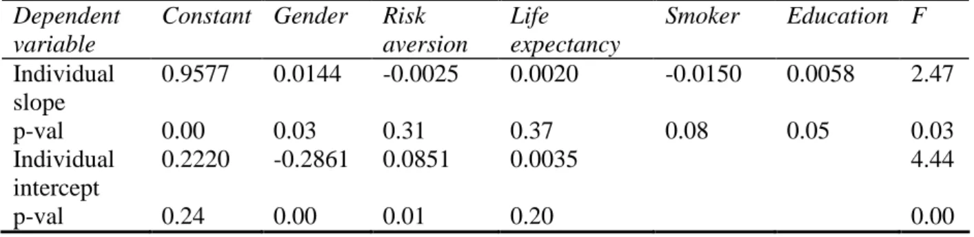
We form the differences in the subjective interest rates for each horizon of 1 year, 5 years, 10 years, 20 years, 30 years and 50 years. These differences are subjective interest rates calculated before and after new information on the true average life expectancy. We cross these differences with individual characteristics. We first used a simple univariate regression and then a system of joint estimate to see whether individual features may explain global moves in attitude toward time preference. The results were negative. None of the individual characteristics appeared to explain changes in attitude toward time. These variables are the individual’s characteristics. A multivariate SUR model of the difference of subjective rates before and after information for horizons of 1, 5, 10, 20, 30 and 50 years was estimated with 5 endogenous variables. This gave the same inconclusive results that no individual characteristics would influence changes in subjective interest rates. The effect of new information on the shape of the term structure of subjective interest rates seems to be random and on average null.

We analyzed directly the influence of information on the value of the two parameters designing the individual term structure data. After information, the average of individual intercepts decreases (50% vs. 53%) and the log of the slope remains on average the same (-3.60% after vs. -(-3.60% before). A t-test of the difference between the intercepts before and