Automatic Estimation of Self-Reported Pain by Interpretable Representations of Motion Dynamics
Texte intégral
Figure
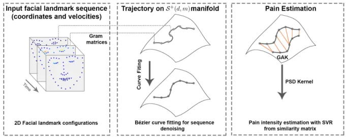
![Fig. 2: Example images from the UNBC-McMaster Shoulder Pain Archive in (a) and (c). In (b) and (d) their corresponding landmark coordinates and velocities, respectively (best viewed in color) [16].](https://thumb-eu.123doks.com/thumbv2/123doknet/12497531.339983/5.892.453.833.234.550/example-mcmaster-shoulder-archive-corresponding-coordinates-velocities-respectively.webp)
Documents relatifs
ZĞƐƵůƚƐ ĨƌŽŵ dĂďůĞ ϰ ĂůƐŽ ƐŚŽǁ ƚŚĂƚ ƚŚĞ ƐĞůĨͲƌĞƉŽƌƚĞĚ ŵĞĂƐƵƌĞ ŝƐ ŵƵĐŚ ůĞƐƐ ƐĞŶƐŝƚŝǀĞ ƚŽ
Proteogenomics and ribosome profiling concurrently show that genes may code for both a large and one or more small proteins translated from annotated coding sequences (CDSs)
L’archive ouverte pluridisciplinaire HAL, est destinée au dépôt et à la diffusion de documents scientifiques de niveau recherche, publiés ou non, émanant des
We first compare the estimation results of intensities of AUs based on the single kernel SVM with different features and the multi-kernel SVM with different fusions of features, as
The following compares the proposed multiscale monogenic optical-flow algorithm presented in this paper, the S¨uhling algorithm, the Zang algorithm and the Felsberg algorithm, which
the same number of 1’s as 2’s and the same number of 0’s as 3’s, and thus there is only one abelian equivalence class.. Before giving the proof, we prove a corollary. The
• Extraction and classification of kinematic features that encode well the dynamics of facial and head movements for the purpose of depression severity level assessment and
According to the above-mentioned issues, we pro- pose in this paper a different approach to measure the bilateral facial asymmetry, when first avoiding the mirror plane detection,
![[PDF] Travaux pratique sur la programmation Android mobile - Free PDF Download](data:image/gif;base64,R0lGODlhAQABAIAAAP///wAAACH5BAEAAAAALAAAAAABAAEAAAICRAEAOw==)