HAL Id: hal-00666748
https://hal.archives-ouvertes.fr/hal-00666748
Submitted on 6 Feb 2012
HAL is a multi-disciplinary open access
archive for the deposit and dissemination of
sci-entific research documents, whether they are
pub-lished or not. The documents may come from
teaching and research institutions in France or
abroad, or from public or private research centers.
L’archive ouverte pluridisciplinaire HAL, est
destinée au dépôt et à la diffusion de documents
scientifiques de niveau recherche, publiés ou non,
émanant des établissements d’enseignement et de
recherche français ou étrangers, des laboratoires
publics ou privés.
Local Visual Patch for 3D Shape Retrieval
Hedi Tabia, Mohamed Daoudi, Jean-Philippe Vandeborre, Olivier Colot
To cite this version:
Hedi Tabia, Mohamed Daoudi, Jean-Philippe Vandeborre, Olivier Colot. Local Visual Patch for 3D
Shape Retrieval. ACM Multimedia Workshop on 3D Object Retrieval 2010, Oct 2010, Florence, Italy.
pp.WS02. �hal-00666748�
Local Visual Patch for 3D Shape Retrieval
Hedi Tabia
LAGIS FRE CNRS 3303 University Lille 1, FranceMohamed Daoudi
LIFL UMR CNRS 8022 Institut TELECOM, FranceJean-Philippe
Vandeborre
LIFL UMR CNRS 8022 Institut TELECOM, FranceOlivier Colot
LAGIS FRE CNRS 3303 University Lille 1, FranceABSTRACT
We present a novel method for 3D-object retrieval using Bag-of-Feature (BoF) approaches [8]. The method starts by selecting and then describing a set of points from the 3D-object. The proposed descriptor is an indexed collection of closed curves in R3on the 3D-surface. Such descriptor has the advantage of being invariant to different transformations that a shape can undergo. Based on vector quantization, we cluster those descriptors to form a shape vocabulary. Then, each point selected in the object is associated to a cluster (word) in that vocabulary. Finally, a BoF histogram count-ing the occurrences of every word is computed. In order to assess our method, we used shapes from the TOSCA and Sumner datasets. The results clearly demonstrate that the method is robust to many kind of transformations and pro-duces higher precision compared with some state-of-the-art methods.
Categories and Subject Descriptors
H.3.1 [Information Storage and Retrieval]: Content Analysis and Indexing; I.5.3 [Pattern Recognition]: Clus-tering
General Terms
Experimentation, Performance, Theory
Keywords
3D Shape, retrieval, curve analysis, bag-of-Features.
1.
INTRODUCTION
Since a few years, there is an increasing interest in analyz-ing shapes of three-dimensional (3D) objects. Advances in 3D scanning technologies, hardware-accelerated 3D graph-ics, and related tools, are enabling access to high quality
Permission to make digital or hard copies of all or part of this work for personal or classroom use is granted without fee provided that copies are not made or distributed for profit or commercial advantage and that copies bear this notice and the full citation on the first page. To copy otherwise, to republish, to post on servers or to redistribute to lists, requires prior specific permission and/or a fee.
3DOR’10,October 25, 2010, Firenze, Italy.
Copyright 2010 ACM 978-1-4503-0160-2/10/10 ...$10.00.
3D data. As technologies are improving, the need for au-tomated methods for analyzing shapes of 3D-objects is also growing. Shape matching remains a central scientific issue for efficient 3D-object search engine design. It plays an im-portant role in many applications such as computer vision, shape recognition, shape retrieval and computer graphics.
In recent years, a large number of papers have been con-cerned in 3D-shape retrieval. Based on the shape descriptors used, existing methods can be classified into two categories: global methods and local methods. For more information about the development of 3D-shape retrieval, we refer the reader to a recent survey [14].
Bag-of-Features (BoF), which is a popular approach in ar-eas of computer vision and pattern recognition, have recently gained great popularity in shape analysis community. Liu et al. [9] presented a 3D-shape descriptor named “Shape Topics” and applied it to 3D partial shape retrieval. In their method, a 3D-object is considered as a word histogram obtained by vector quantizing Spin images of the object. Ohbuchi et al. [10] introduced a view-based method using salient local features. They represented 3D-objects as word histograms derived from the vector quantization of salient local descriptors extracted on the depth-buffer views cap-tured uniformly around the objects. Ovsjanikov et al. [11] presented an approach to non-rigid shape retrieval similar in its spirit to text retrieval methods used in search engines. They used the heat kernel signatures to construct shape de-scriptors that are invariant to non-rigid transformations.
Inspired by the work presented in [11] and with analogy to methods using the bag-of-words representation for text retrieval [3], we propose a new visual similarity based 3D-shape retrieval approach. An overview of the method is detailed in section 2. Section 3 presents the experimental results. Conclusion and future work end the paper.
2.
THE METHOD
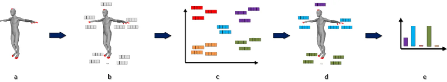
The general steps for building a BoF representation for 3D-objects are depicted in Figure 1. It starts by selecting (step a) and then describing (step b) a set of points from the 3D-object. The selection can be done in various ways, the most typical being the application of interest point selection algorithm. The proposed descriptor is an indexed collection of closed curves in R3on the 3D-surface. Such descriptor has the advantage of being invariant to different transformations that a shape can undergo.
Figure 1: An illustration of our method. a) 3-D object feature extraction b) 3-D local patch construction c) vector quantizing d,e) a word histogram
Given a set of descriptors, the next step (step c) is to cluster those points to form the vocabulary by quantization. Then, each point selected in the object is associated to a “word” (i.e. a cluster) in the shape vocabulary (step d) and the BoF histogram counting the occurrences of every word is computed (step e). Algorithm 1 summarizes this process. Algorithm 1 : Pseudo-code for building a BOF represen-tation for 3D-objects.
for all 3D-object do
pointsDesc ←− FeatureExtraction(3D-object) end for
vocab ←− quantizePoints(pointsDesc) for all 3D-object do
bofs ←− computeHistogram(vocab, pointsDesc) end for
Func FeatureExtraction(3D-object), return descriptors pointsPos ←− FeaturePointExtraction(3D-object) descriptors ←− CurveDescriptors(3D-object, pointsPos)
return descriptors end Func
2.1
Feature point extraction
Feature points are characteristic of the shape and corre-spond to points of geometrical and perceptual interests in 3D-objects. These points are the reference points for our analysis. They are extracted using Tierny et al.’s method [15]: extremities of prominent components are identified by intersecting the sets of extrema of two scalar functions based on the geodesic distances between the two furthest vertices on the surface mesh representing the 3D-object. The extrac-tion is invariant to isometric transformaextrac-tions and robust to noise. Figure 1 (step a) shows the localization of feature points extracted from a human 3D-object.
2.2
Curve descriptors
As mentioned earlier, the proposed descriptor is a collec-tion of closed curves. These curves are extracted around each feature point previously extracted. The descriptor in-trinsically invariant is able to capture the geometry of ob-ject patches using the geometries of the associated curves. Curves are defined as level curves of an intrinsic distance function on the 3D-part surface. Their geometries in turn are invariant to the rigid transformations of the 3D-part sur-face. These curves jointly contain all the information about the surface and it is possible to go back-and-forth between the surface and the curves without any ambiguity. In order to study the geometry of curves, we used Riemannian met-rics on curve spaces and we adopt the Joshi et al’s approach
[5] because it simplifies the elastic shape analysis. The main steps are: (i) define a space of closed curves of interest, (ii) impose a Riemannian structure on this space using the elastic metric, and (iii) compute geodesic paths under this metric. These geodesic paths can then be interpreted as optimal elastic deformations of curves.
We start by considering a closed curve β in R3. Since it is a closed curve, it is parameterizable using β : S1
→ R3. We will assume that the parameterization is non-singular, i.e. k ˙β(t)k 6= 0 for all t. The norm used here is the Eu-clidean norm in R3. Note that the parameterization is not assumed to be arc-length; we allow a larger class of param-eterizations for improved analysis. To analyze the shape of β, we shall represent it mathematically using a square-root velocity function (SRVF), denoted by q(t), according to: q(t)=. √β(t)˙
k ˙β(t)k.
q(t) is a special function that captures the shape of β and is particularly convenient for shape analysis, as we de-scribe next. Firstly, the squared L2-norm of q, given by: kqk2=R
S1hq(t), q(t)i dt = R
S1k ˙β(t)kdt , which is the length of β. Therefore, the L2-norm is convenient to analyze curves of specific lengths. Secondly, as shown in [5], the classical elastic metric for comparing shapes of curves becomes the L2-metric under the SRVF representation. This point is very important as it simplifies the calculus of elastic met-ric to the well-known calculus of functional analysis un-der the L2-metric. In order to restrict our shape analy-sis to closed curves, we define the set: C = {q : S1 → R3|RS1q(t)kq(t)kdt = 0} ⊂ L
2
(S1, R3) . Here L2(S1, R3) denotes the set of all functions from S1
to R3that are square integrable. The quantity R
S1q(t)kq(t)kdt denotes the total displacement in R3 as one traverses along the curve from start to end. Setting it equal to zero is equivalent to having a closed curve. Therefore, C is the set of all closed curves in R3, each represented by its SRVF. Notice that the elements of C are allowed to have different lengths. Due to a non-linear (closure) constraint on its elements, C is a nonnon-linear manifold. We can make it a Riemannian manifold by using the metric: for any u, v ∈ Tq(C), we define:
hu, vi = Z
S1
hu(t), v(t)i dt . (1) We have used the same notation for the Riemannian met-ric on C and the Euclidean metmet-ric in R3 hoping that the difference is made clear by the context. For instance, the metric on the left side is in C while the metric inside the integral on the right side is in R3. For any q ∈ C, the tan-gent space: Tq(C) = {v : S1→ R3| hv, wi = 0, w ∈ Nq(C)} , where Nq(C), the space of normals at q is given by: Nq(C) =
span{kq(t)kq1(t)q(t) + kq(t)ke1, q2(t)
kq(t)kq(t) + kq(t)ke 2, q3(t)
kq(t)kq(t) + kq(t)ke3} , and where {e1, e2, e3} form an orthonormal basis of R3.
It is easy to see that several elements of C can represent curves with the same shape. For example, if we rotate a curve in R3, we get a different SRVF but its shape remains unchanged. Another similar situation arises when a curve is re-parameterized; a re-parameterization changes the SRVF of curve but not its shape. In order to handle this vari-ability, we define orbits of the rotation group SO(3) and the re-parameterization group Γ as the equivalence classes in C. Here, Γ is the set of all orientation-preserving dif-feomorphisms of S1 (to itself) and the elements of Γ are viewed as re-parameterization functions. For example, for a curve β : S1 → R3
and a function γ : S1 → S1, γ ∈ Γ, the curve β(γ) is a re-parameterization of β. The corre-sponding SRVF changes according to q(t) 7→p ˙γ(t)q(γ(t)). We set the elements of the set: [q] = {p ˙γ(t)Oq(γ(t))|O ∈ SO(3), γ ∈ Γ} , to be equivalent from the perspective of shape analysis. The set of such equivalence classes, denoted by S = C/(SO(3) × Γ) is called the shape space of closed. curves in R3. S inherits a Riemannian metric from the larger space C and is thus a Riemannian manifold itself. The main ingredient in comparing and analyzing shapes of curves is the construction of a geodesic between any two elements of S, under the Riemannian metric given in Eqn. 1. Given any two curves β1 and β2, represented by their SVRFs q1 and q2, we want to compute a geodesic path between the orbits [q1] and [q2] in the shape space S. This task is accomplished using a path straightening approach which was introduced in [7]. The basic idea here is to connect the two points [q1] and [q2] by an arbitrary initial path α and to iteratively update this path using the negative gradient of an energy function E[α] = 12R
sh ˙α(s), ˙α(s)i ds. The interesting part is that the gradient of E has been derived analytically and can be used directly for updating α. As shown in [7], the critical points of E are actually geodesic paths in S. Thus, this gradient-based update leads to a feature point of E which, in turn, is a geodesic path between the given points. We will use the notation d(β1, β2) to denote the geodesic distance, or the length of the geodesic in S, between the two curves β1 and β2.
We extend the curve distance analyzing procedure to com-pute a distance between patches. Let D denotes the global distance between two patches. Given any two surfaces patches P1and P2, and their collection of curves {βλ1, λ ∈ [0, L]} and {β2
λ, λ ∈ [0, L]}, respectively, we compare the curves β 1 λand β2
λ, and we accumulate these distances over all λ values. Formally, we define a distance: D : C[0,L]× C[0,L]
→ R≥0, given by D(P1, P2) = Z L 0 d(βλ1, β 2 λ)dλ. (2)
2.3
Shape vocabulary construction
In our method, the vocabulary is a way of construct-ing a feature vector for classification that relates descrip-tors in 3D-object query to descripdescrip-tors of 3D-objects in the database. One extreme of this approach is to compare each query descriptor to all indexed descriptors: this seems im-practical given the huge number of indexed descriptors in-volved. Another extreme is to try to identify a small num-ber of large “clusters” that are good at discriminating a
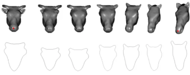
Figure 2: Geodesic path between two curves (last level) of cowhead part and horse-head part
given class. Most clustering or vector quantization algo-rithms are based on iterative square-error partitioning or on hierarchical techniques. Square-error partitioning algo-rithms attempt to obtain the partition which minimizes the within-cluster scatter or maximizes the between-cluster scat-ter. Hierarchical techniques organize data in a nested se-quence of groups which can be displayed in the form of a tree. They need some heuristics to form clusters and hence are less frequently used than square-error partitioning tech-niques in pattern recognition. In our case we chose to use the simplest square-error partitioning method: k-means [4]. This algorithm proceeds by iterated assignments of points to their closest cluster centers and re-computation of the cluster centers. The centers of cluster are 3D-patch whose parameter values are the mean of the parameter values of all the patches in the cluster. To calculate mean of 3D-patches parametrized by curves, we use Karcher means [12]. In fact, the Riemannian structure defined on the manifold of 3D-patch surfaces enables us to perform some statistical analysis for computing 3D-surfaces mean and variance. The Karcher mean is based on the intrinsic geometry of the man-ifold to define and compute a mean on that manman-ifold. It is defined as follows. Let D(Pi, Pj) denotes the length of the geodesic from Pi to Pj. To calculate the Karcher mean of 3D-patch surfaces {P1, ..., Pn}, we define the variance func-tion ϑ : C[0,L]−→ R, ϑ(P ) =Pn
i=1D(P, Pi) 2
. The Karcher mean is then defined by :
T = argminP ∈C[0,L]ϑ(P ) (3)
The intrinsic mean may not be unique, i.e. there may be a set of points in C[0,L]for which the minimizer of ϑ is ob-tained. To interpret geometrically, T is an element of C[0,L], that has the smallest total deformation from all given 3D-patch surfaces. The final set of Karcher means represents the codebook. Each element in this codebook is called a keyshape.
Figure 3 shows the shape of the Karcher mean of four 3D-objects. The mean shape is located at the center of the figure.
2.4
Shape histogram computing
The final step of the BoF method is the computing of the dissimilarity between two objects. To this end, we compute the cumulative occurrences of keyshapes in both objects. Curve descriptors in the 3D-objects are assigned to the near-est neighbor keyshapes in the codebook. Then each object is represented using an histogram whose ithbin contains the number of ithkeyshapes in that object. Finally, the dissim-ilarity between two objects can be computed using several
Figure 3: The shape of the Karcher mean of four 3D-objects and its associated sets of curves
metrics, as DM ax, DM in, etc. We use the L2 distance to measure the distance between two objects.
3.
EXPERIMENTS
In this section, we present the experimental results, some state-of-the-art shape-matching algorithms to compare with. The robustness to shape deformations is discussed in the sequel. The algorithms, described in the previous sections, have been implemented using Matlab software. The frame-work encloses an off-line feature extraction algorithm and a vector quantization algorithm, and an on-line retrieval pro-cess.
The proposed approach has been tested on database com-posed of shapes from the TOSCA and the Sumner datasets. The TOSCA dataset has been proposed by Bronstein et al. [1] for non-rigid shape correspondence measures. The Sum-ner dataset has been proposed by SumSum-ner and Popovic [13] for deformable shape correspondence. The total set size is 450 shapes.
3.1
Results
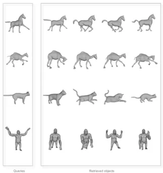
In order to assess our method, we performed shape re-trieval experiments. From a qualitative point of view, Fig-ure 4 gives a good overview of the framework efficiency. This figure visualizes some examples of retrieved objects, ordered by relevance, which is inversely proportional to the distance from the query. We can note, in this figure, all top-results are relevant to the queries.
3.2
Comparison with related work
From a more quantitative point of view, we compare the Precision vs Recall plot of our approach with some well-known stat-of-the-art methods:
• Spherical Harmonic Descriptor (SHD) [6]. A method describing a 3D-object as a feature vector consisting of spherical harmonic coefficients extracted from three spherical functions giving the maximal distance from center of mass as a function of spherical angle. • LightField Descriptor (LFD) [2]. A well-known
view-based 3D-retrieval method. 10 silhouettes are used to describe a 3D-object.
Figure 4: Retrieved results, ordered by relevance, using our method
Figure 5: Precision vs Recall plots for the proposed method and some state-of-the-art methods
Figure 5 shows the Precision vs Recall plots. Such a plot is the average of the set of Precision vs Recall plots corre-sponding to the models of the query-set. As the curve of our approach is higher than the other ones, it is obvious that it outperforms related methods.
3.3
Robustness under shape deformations
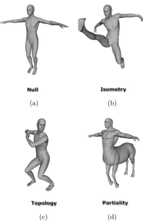
In this section, we discuss the robustness of the retrieval method under deformed instances of the query shapes. For this end, we conduct similar experiments as in [11]. First, we choose shapes in one of the four transformation categories (shown in Figure 6) as a query set, and we kept the remain-ing transformation with the objects in the dataset. The re-sults of this experiment are shown in Figure 7 as Precision vs Recall plots. The method is robust under isometry and par-tiality deformations, however it is less robust to topological ones. This is due to the feature point extraction step of the framework, which is based on geodesics. In practice, with the TOSCA and the Sumner datasets, feature extraction
(a) (b)
(c) (d)
Figure 6: Examples of some transformations of 3D-object
turns out to be homogeneous within most classes. However, the geodesic metric is known to be very sensitive to topology changes which makes the overall framework quite sensible to topology variations as well.
4.
CONCLUSIONS
In this paper, we have presented a novel method for re-trieving 3D-objects based on a BoF approach. We have pro-posed a new feature extraction algorithm based on curve analysis. We have presented results for retrieving 3D-objects from the TOSCA and the Sumner datasets. These results show the effectiveness of our approach and clearly demon-strate that the method is robust to non-rigid and deformable shapes.
5.
REFERENCES
[1] A. Bronstein, M. Bronstein, and R. Kimmel. Efficient computation of isometry-invariant distances between surfaces. IEEE Trans. VCG, 13/5:902–913, 2007. [2] D.-Y. Chen, X.-P. Tian, Y.-T. Shen, and
M. Ouhyoung. On visual similarity based 3D model retrieval. Eurographics, 22:223–232, 2003.
[3] N. Cristianini, J. Shawe-Taylor, and H. Lodhi. Latent semantic kernels. Journal of Intelligent Information Systems, 18:127–152, 2002.
[4] O. Duda, P.-E. Hart, and D.-G. Stork. Pattern classification. In John Wiley Sons, 2000.
[5] S. Joshi, E. Klassen, A. Srivastava, and I. Jermyn. Removing shape-preserving transformations in
Figure 7: Precision vs Recall plots for some classes of shape transformations
square-root elastic (sre) framework for shape analysis of curves. In EMMCVPR, pages 387–398, 2007. [6] M. Kazhdan, T. Funkhouser, and S. Rusinkiewicz.
Rotation invariant spherical harmonic representation of 3d shape descriptors. Geometry Processing, Aachen, Germany, 2003.
[7] E. Klassen and A. Srivastava. Geodesics between 3d closed curves using path-straightening. In European Conference on Computer Vision (ECCV), pages 95–106, 2006.
[8] Z. Lian, A. Godil1, and X. Sun. Visual similarity based 3d shape retrieval using bag-of-features. In International Conference on Shape Modeling and Applications (SMI), 2010.
[9] Y. Liu, H. Zha, and H. Qin. Shape topics: A compact representation and new algorithms for 3d partial shape retrieval. In Computer Society Conference on Computer Vision and Pattern Recognition, 2006. [10] R. Ohbuchi, K. Osada, T. Furuya, and T. Banno.
Salient local visual features for shape-based 3d model retrieval. In International Conference on Shape Modeling and Applications (SMI), 2008.
[11] M. Ovsjanikov, A.-M. Bronstein, M.-M. Bronstein, and L.-J. Guibas. Shapegoogle: a computer vision approach for invariant shape retrieval. In Workshop on Nonrigid Shape Analysis and Deformable Image Alignment (NORDIA), 2009.
[12] C. Samir, A. Srivastava, M. Daoudi, and E. Klassen. An intrinsic framework for analysis of facial surfaces. International Journal of Computer Vision, Avril 2009. [13] R. Sumner and J. Popovic. Deformation transfer for
triangle meshes. In International Conference on Computer Graphics and Interactive Techniques, 2004. [14] J. W.-H. Tangelder and R.-C. Veltkamp. A survey of
content based 3d shape retrieval methods. Multimedia Tools and Applications, 39(3):441–471, September 2008.
[15] J. Tierny, J.-P. Vandeborre, and M. Daoudi. Partial 3D shape retrieval by reeb pattern unfolding.
Computer Graphics Forum - Eurographics Association, 28:41–55, March 2009.