Assessing the severity of diatom deformities using geometric morphometry Angélique Cerisier1, Jacky Vedrenne1, Isabelle Lavoie2, Soizic Morin1
1
Irstea, UR EABX, 50 avenue de Verdun, 33612 Cestas cedex, France
2
INRS, Centre ETE, 490 rue de la Couronne, G1K 9A9 Québec, Canada
Abstract
Deformities in diatoms are increasingly used as an indicator of toxic stress in
freshwaters. However, the percentage of deformities alone often fails at highlighting the magnitude of toxic exposure. It has been suggested that the severity of the deformation (degree of departure from normal form) could be a valuable aspect to consider in addition to the percentage of deformities in an assemblage. An approach combining the assessment of deformities coupled with information on their severity could improve the sensitivity of this biomarker.
With the aim of quantifying the deviation from the normal form, we tested the applicability of geometric morphometry to evaluate the degree of deformities in different diatom species. We used photomicrographs of normal and deformed
specimens from laboratory cultures of Gomphonema gracile, Nitzschia palea, and of Achnanthidium minutissimum from field samples collected along a gradient of toxic contamination. The geometric morphometry approach is based on several landmarks positioned on the outline of the diatom valves, followed by a Procrustes
superimposition analysis to determine shape variations.
Statistical analyses were conducted based on the geometrical coordinates of the landmarks. This technique allowed to discriminate between normal and deformed individuals. The geometric morphometry approach revealed a gradient in the intensity of the deformities observed on Gomphonema gracile and Achnanthidium
minutissimum, in-line with a priori, visually-determined (subjective) classifications. A relationship between the degree of deformity in Achnanthidium minutissimum and a gradient of zinc contamination was found. In contrast, the approach failed to obtain good fit for Nitzschia palea individuals because deformities in this species were more variable in terms of their location on the valves.
Geometric morphometry provided encouraging results to objectively quantify the intensity of diatom deformities affecting valve outline, and could easily be
implemented in further automatic diatom identification developments.
1. Introduction :
Anthropogenic activities such as industrialization, urbanization and intensive agriculture, are involved in the degradation of freshwater ecosystems through the generation of diffuse or point source pollution. Water quality programs based on biotic indicators are being implemented worldwide to monitor aquatic ecosystems with the aim of improving their management and ultimately, achieving better
ecological status. In Europe, the Water Framework Directive (2000/06/EC) classifies the ecological status of waterbodies based on several biological quality elements, including diatoms (Kelly et al. 2009; Kelly et al. 2012). Routinely used diatom indices have been developed in Europe and elsewhere to assess general water quality, mainly reflecting nutrient enrichment, organic matter and conductivity (Coste et al. 2009; Lavoie et al. 2014). However, these indices were not modeled to include the assessment of contamination by toxicants. Over the last decades, special attention has been paid to diatom deformities (Falasco et al. 2009a; Lavoie et al. 2017; Morin et al. 2012) as indicators of freshwater impairment by toxic compounds, particularly metals and pesticides. To better account for this type of environmental stress, Coste et al. (2009) included the percentage of deformed diatoms in the Biological Diatom Index to improve its sensitivity to toxicants, where high numbers of teratologies equate to a lower index score (indicating lower water quality). Lavoie et al. (2017), however, questioned the ecological meaning of simply using the overall total
percentage of teratologies as a unique indication of a response to a toxic stress. In their review, they argue that not all species may be equally prone to deformities, and that the type of deformity observed may represent valuable ecological information to consider. Lavoie et al. (2017) also point out the problem relative to subjectivity when assessing the presence of teratologies (what is considered as abnormal), as well as the variability that may be introduced when multiple analysts (microscopists) are involved. This aspect could be of even higher interest if the degree (“severity”) of the deformity brings additional information about the level of stress experienced by the diatoms, which could then also represent a metric worth integrating to the
assessment.
Based on the above-mentioned uncertainties potentially affecting the assessment of toxic stresses using deformities as a biological descriptor, it is obvious that there are still many gaps to fill in order to fully and appropriately interpret the ecological signal provided by abnormal diatoms. In recent years, there have been studies conducted with the aim of addressing some of the limitations related to the approach. For example, Fernández et al. (2018) presented the Metal Pollution Index (ICM), using a refined method associating specific scores to deformed specimens of different species, based on their distribution in metal-polluted sites in rivers of Southwestern Spain. These scores may reflect, at least indirectly, the proneness of various species to deformity. Other studies classified observed abnormal forms into different types of deformities (Arini et al. 2013; Falasco et al. 2009b; Pandey et al. 2014), but did not discuss the added value of considering this information. Except for a minority of studies, most publications on the subject rely only on overall percentage (%) of
deformities, and this may be the reason for the lack of correlation often observed with the gradients in environmental stresses, particularly for field conditions. More
research on the eco(toxico)logical signal provided by different types of diatom deformities is clearly needed, as the presence of teratologies is a metric that is growing in popularity for bioassessment purposes.
In their review and discussion on the use of teratologies in bioassessment, Lavoie et al. (2017) called for more research on various aspects related to deformities, such as an approved method for determining if a specimen deviates enough from its expected form to be considered as ‘’abnormal’’, and for objectively assessing the degree or severity of the aberrations. Hypothesizing that the degree of deformity could be an indicator of contamination level, this paper takes up the challenge of proposing a method to objectively assess the deviation from normality. The approach is based on geometric morphology, which has been previously used successfully by Olenici et al. (2017) to evidence variations in deformities affecting the outline of Achnanthidium species from a Romanian stream exposed to acid mine drainage. This image-based approach relies on the changes in the location of landmarks positioned along the valve outline and/or on specific features (intersection between internal structures). It is a widely-used method for larger organisms such as chironomids (Arambourou et al. 2014), drosophila (Debat et al. 2003), and fish (Avigliano et al. 2017). It has also been used to discriminate between morphologically closely-related diatoms
(Fránková et al. 2009; Pappas et al. 2014; Potapova and Hamilton 2007; Woodard et al. 2016). Olenici et al. (2017) demonstrated the relevance of this approach in
highlighting a deformity gradient of teratological Achnanthidium minutissimum species. Moreover, they found a positive relationship between the degree of deviation in valve outline and dissolved zinc concentrations, confirming the hypothesis made by Lavoie et al. (2017) that the severity of the deformity could provide valuable additional information worth considering. However, in the work presented by Olenici et al. (2017), a high number of landmarks (40 per individual) were positioned to perform the analysis, resulting in a long processing time for large sets of images.
With the aim of assessing the wider applicability of the geometric morphometry approach to measure the degree of deformities in diatoms, we used three common benthic diatom species found with high percentages of deformation, in which a gradient of shape variation was visually observable. Given the time needed to position the landmarks, we tested the possibility of using a limited number of
landmarks, without losing discrimination power in the analysis. For the three species tested, we assessed the ability of the geometric morphometry analysis: i) to
discriminate between normal and deformed morphotypes, and ii) to provide evidence of a gradient in intensity (severity) of the deformities.
2. Materials and Methods 2.1. Biological material
Three common species of diatoms were used for this study: Gomphonema gracile Ehrenberg, Nitzschia palea Kützing (W. Smith) and Achnanthidium minutissimum (Kützing) Czarnecki. These benthic, pennate diatoms are widely distributed in temperate streams and have contrasting ecological preferences. Omnidia codes (Lecointe et al. 1993) provided at https://hydrobio-dce.irstea.fr/telecharger/diatomees-ibd/ were used to refer to these species: GGRA and GGRT for normal and abnormal morphotypes of G. gracile, NPAL and NPTR for normal and abnormal morphotypes of N. palea, and ADMI and ADMT for normal and abnormal morphotypes of A. minutissimum.
Gomphonema gracile specimens were collected from laboratory monospecific cultures (Irstea, France) of the same age and origin (Coquillé et al. 2015; Coquillé and Morin, unpublished data), but that diverged morphologically over time. This species is acidophilic and sensitive to degraded water quality (Coste et al. 2009). GGRA specimens were 21.9±1.9 µm long, 5.9±0.5 µm wide, and slightly heteropolar. GGRT individuals were larger, with a length of 33.9±2.1 µm and a width of
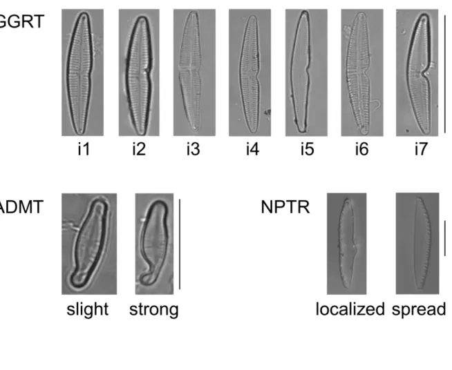
6.2±0.4 µm. Deformities noted on GGRT were consistently characterized as a marked invagination on the side opposite to the sigma, producing a “boomerang shape” (Figure 1).
Nitzschia palea specimens were collected from a monospecific culture used for an exposure experiment (INRS-ETE, Quebec), where cells were exposed to different concentrations of cadmium (Kim Tiam et al. in press). Although NPAL is regarded as tolerant to various environmental pressures (e.g. eutrophication, metal and organic contamination, salinization), an average of 3.6% deformed individuals (NPTR) were found under Cd stress (Kim Tiam et al. in press). N. palea specimens were
26.2±2.1 µm long and 4.5±0.5 µm wide. Several types of deformities were observed (shape, abnormal raphe canal, interruption in the fibulae), but only aberrations in the valve outline were considered for the purpose of the present study. Irregular outlines were characterized by a bump on one site of the valve. More information on the nature of the various types of deformities noted on NPTR exposed to Cd can be found in Kim Tiam et al. (in press), in which photomicrographs are also available. Finally, we used photomicrographs of Achnanthidium minutissimum from field samples collected on different sampling occasions (2009, 2012, 2013 and 2014), downstream of an industrial plant releasing toxic effluents (500 and 4500 m, respectively Down1 and Down2 in Lainé et al. 2014). ADMI is a pioneer species, generally indicative of good water quality (Coste et al. 2009) but also found in streams exposed to high toxic pressure (eg. Lainé et al. 2014; Leguay et al. 2016). ADMI and ADMT were of smaller sizes than the other two species considered in this study, with an average length of 10.1±1.8 µm. Up to 13% of ADMT were found at Down2 in 2014 (Morin et al. 2014). The deformity in ADMT was a typical invagination
at its apex (sometimes at both apices), referred to as a cymbelliclinum-like teratology in Cantonati et al. (2014).
2.2. Photomicrograph acquisition and visual classification
Diatom samples were cleaned with H2O2 to remove organic material and mounted
onto permanent slides using Naphrax (Brunel Microscopes Ltd) following the standard protocol EN 13946 (2014). Photomicrographs were obtained using 1000x magnification observations under optical microscopes equipped with image
acquisition systems.
Only the best resolution photomicrographs of valves resting flat on the microscope slide were selected for the analysis. The specimens illustrated on the
photomicrographs were visually (subjectively) classified into “normal” or “abnormal” categories, based on whether or not they presented the “expected” symmetrical outline. A total of 269 specimens of Gomphonema gracile (130 GGRA and 139 GGRT), 49 of Nitzschia palea (21 NPAL and 28 NPTR) and 335 of Achnanthidium minutissimum (189 ADMI and 146 ADMT) were analyzed. The GGRT population exhibited a wide range in the severity of the teratologies. Due to the large size of the specimens, they were easily a priori attributed a deformity index based on visual observations of shape variations (Figure 1). This classification was used to further examine the compliance between visual and landmark-based assessment of deformity gradients.
2.3. Geometric morphometry and statistical analyses
To apply the geometric morphometry approach to the photomicrographs, the position and number of landmarks on the valve contour was first optimized (more details in Supplemental material). Landmarks represent homologous loci that are present on all studied specimens. Here, we selected inflection points, and complementary
landmarks were placed at a fixed distance from these points. In this study, a fixed number of landmarks (6 for G. gracile; 7 for A. minutissimum; 16 for N. palea) were positioned as shown in Figure 2, and digitized using the freely distributed program tpsDig232 (Rohlf 2010). The generalized orthogonal least-square Procrustes method was applied (Rohlf and Slice 1990) to overcome differences in cell size, position on photomicrographs and orientation between individuals. The different individual
configurations were scaled using the “centroid size”, then superimposed and rotated. Using the final geometrical coordinates of the landmarks, a Thin-Plate Spline (TPS) was performed using tpsRelw32 (Rohlf 2010). The Relative warps (RW) scores on the TPS (i.e. axes coordinates) for individuals with different morphotypes or degree of deformity were then compared using ANOVAs, followed by Tukey tests, under the R environment (Ihaka and Gentleman 1996).
3. Results and Discussion
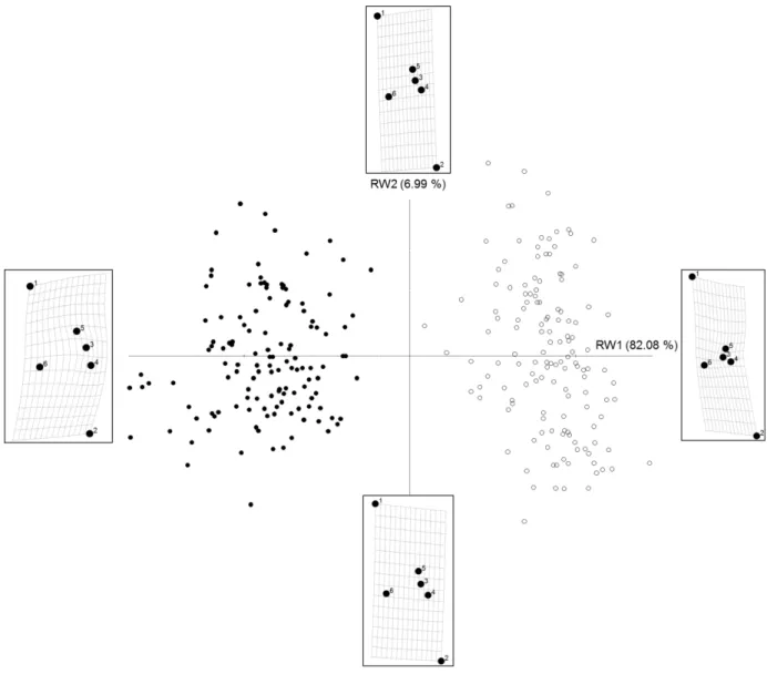
3.1. Quantifying the severity of outline deformities in Gomphonema gracile cultures Figure 3 highlights the ability of the geometric morphometry approach to efficiently discriminate normal from deformed G. gracile specimens, using a limited set of six landmarks. Indeed, RW1, which is the most discriminating axis (82 % of the variability explained), was directly linked to deformation presence or absence. All normal
individuals clustered on the left-hand side panel (negative values of RW1), well separated form deformed specimens, which clustered on the right-hand side panel (positive values of RW1). Moreover, the more positive the coordinates on RW1, the more severe or marked the deformities were. Interestingly, RW2 (explaining 7 % of the variability) was related to shape variations that were not considered as
deformities, but rather to different length-to-width ratios, where the most elongated forms were found at the top of the graph (positive values of RW2). The diatoms used for this study diverged morphologically from the normal form after being maintained in culture conditions for one year. The cell dimensions of GGRA individuals continued to decrease compared to the diatom that was originally isolated, while GGRT still
presented a larger initial size (Coquillé and Morin, unpublished data). Dimensions alone did not play a role in the discrimination between morphotypes, as the
Procrustes method includes a rescaling step. The dissymmetry in outline was found to be the major driver in the TPS analysis, highlighting the discrimination power of the method, even with a much lower number of landmarks than was originally used by Olenici et al. (2017).
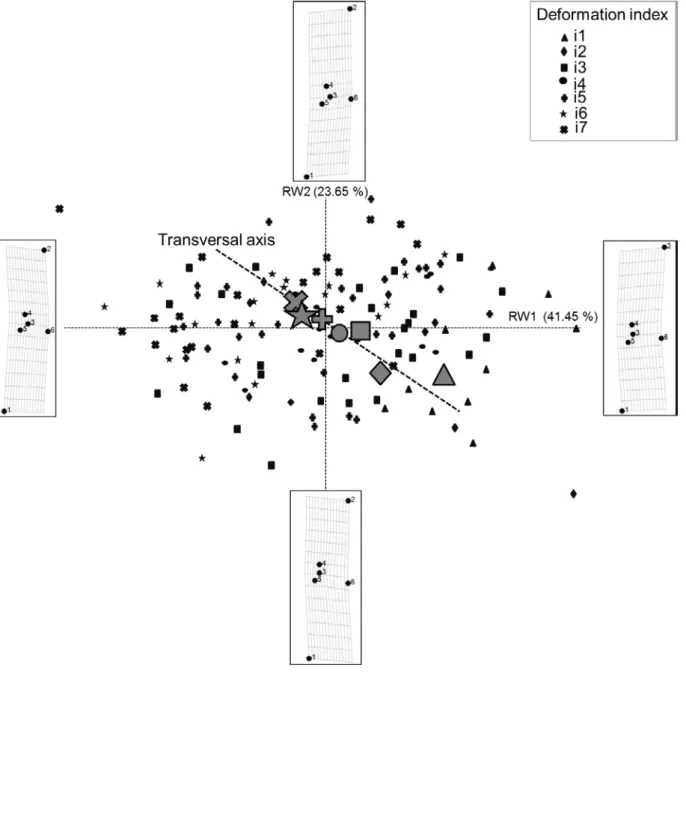
To refine the morphometry analysis of the teratological valves (GGRT), a new TPS was performed using only GGRT individuals (Figure 4), labelled according to the deformation index to which they were a priori visually (subjectively) assigned (Figure 1). The first axis (RW1, accounting for 41 % of the variability, Figure 4) mostly
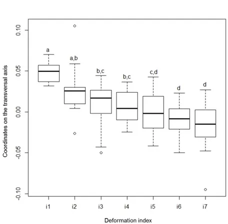
reflected the curvature of the valve, while RW2 (24 %) was more closely related to the depth of the invagination. As the severity of this “boomerang-shaped” teratology is a combination of both more pronounced curvature and stronger invagination, the gradient of teratology severity was best observed along a transverse axis, where less-deformed diatoms (indices 1 to 4) were located in the lower right panel, and the most deformed diatoms (indices 6 and 7) clustered in the top left panel (Figure 4). This result demonstrates the ability of the geometric morphometry method to detect a gradient in deformations, confirming the visually-performed a priori classification. The coordinates of the individuals along the transverse axis were calculated a posteriori from their coordinates on RW1 and RW2, using geometrical formulae. Figure 5 clearly shows that the position of each individual on the ordination, classified based on increasing “deformity classes” along this transversal axis, provides an objective quantification of deformation severity (with statistical differences showed by an ANOVA and a Tukey test). The overlap between neighboring indices shows continuity in the morphological variation gradient, but statistical differences were
found between the more distant indices, indicating that the TPS allowed for discrimination among certain levels of severity.
3.2. Outline deformities in Nitzschia palea cultures exposed to cadmium
The first two axes of the TPS analysis performed on Nitzschia palea specimens explained 39 % (RW1) and 26 % (RW2) of the variability, respectively (Figure 6). Both axes were related to valve asymmetry and differences in the length-to-width ratio, with larger diatoms positioned at positive values of RW1 and RW2. RW1
successfully discriminated between NPAL and NPTR individuals (ANOVA followed by Tukey test, p<0.05), with the normal and deformed N. palea specimens respectively clustered on the right and left-hand side of the graph, respectively. Adding specimens to this analysis would have been desirable to strengthen the results, but it should be noted that teratological specimens (in both monocultures and in assemblages) are rarely found in high abundance, even when exposed to toxic stress (e.g. Morin et al., 2012; Lavoie et al., 2017). Moreover, some species, such as G. gracile (e.g. Morin and Coste 2006) always exhibit similar outline aberrations, while others such as N. palea display a large array of potential deformities, not necessarily affecting valve outline. For this reason, only a limited number of photomicrographs were available to examine shape deformities on N. palea using the material from Kim Tiam et al. (in press), but the discrimination power we obtained based on about 50 N. palea specimens is nevertheless encouraging for further use in ecotoxicological assessment.
Considering only outline teratologies in NPTR individuals, the analysis failed to properly highlight any deformity gradient. This result may be the consequence of several limitations of the analysis performed on this species. First, the low number of individuals available allowed for the separation of the photomicrographs into no more than two categories. Second, the location and aspect of the bulge; it should be
mentioned that the bump on NPTR was not consistently positioned in the same area of the valve side, and was sometimes well-defined, while sometimes spread-out over the valve side. This rendered difficult the positioning of the landmarks to account for all different deformity scenarios.
3.3. Assessing deformity gradients in populations of Achnanthidium minutissimum from field samples
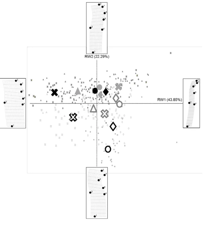
The first axis of the TPS conducted on Achnanthidium minutissimum individuals (RW1, accounting for 44 % of the variability) was related to the length to width ratio, with larger diatoms located in the left-hand side panel (Figure 7). The second axis (RW2, accounting for 22 % of the variability) reflected a deformity gradient where normal diatoms were found along the positive values of the axis, while the most
negative values were related to marked cymbelliclinum-like outlines. Interestingly, the normal and deformed diatoms from the same samples (site and year) were arranged similarly on the TPS, except for Down1 in 2013, probably because only 2 deformed individuals were considered. In fact, the coordinates of the deformed diatoms were systematically higher on RW1 and lower on RW2, highlighting the deformity
(invagination, on RW2) and its impact on the overall length to width ratio. This consistency in sample arrangement on the TPS suggests that the deformed
individuals were a sub-population of the normal ones. Moreover, the severity of the deformity was site dependent: diatoms from Down2 were generally more severely deformed than those collected immediately downstream of the industrial effluents (Down1).
The severity of the deformity was also variable depending on the year of sampling. In particular, deformity intensity observed on ADMT collected at Down2 was ranked as follows: 2014>2012>2013. At Down1, the deformities were ordered as follows: 2013>2009>2014>2012. It should be noted that a lower number of individuals per year (2 to 5) were considered at Down1 (except for 2009), compared with Down2 (34 to 36 individuals). This gradient in deformity intensity (RW2 sample coordinates) was partly explained by increasing dissolved metals, in particular zinc concentrations (R²=0.21, p-value<0.01). This is consistent with previously reported correlations between zinc exposure and increasing numbers and severity of deformities in A. minutissimum (Cantonati et al. 2014; Olenici et al. 2017). Olenici et al. (2017) also used the geometric morphometry approach to develop an indicator of deformity level based on partial TPS warps. The results from the present study converge with their observations and conclusions on the value of using this method as a way to
objectively assess and quantify diatom deformities.
3.4. Advantages and limitations of morphometric geometry to quantify the severity of diatom deformities
Morphometric geometry is proving to be a useful method to evaluate the severity of diatom deformities (Olenici et al. 2017; this study). For the first time here, we were able to correlate a gradient in deformity level based on geometrical coordinates of the samples on the TPS with an a priori established classification of the gradient based on visual observation (for G. gracile and A. minutissimum). Hypothesizing that the degree of deformity could be an indicator of the intensity of micropollutant pollution, characterizing the severity of shape-related deformities may improve diatom-based ecotoxicological assessments as suggested in Lavoie et al. (2017).
In this study, several advantages of morphometric geometry are highlighted. Firstly, the approach allows for the discrimination between normal and deformed specimens of the three species tested. This method had already proved its usefulness in
differentiating subtle shape variations (between species) that were hardly discernible by the human eye (Potapova and Hamilton 2007; Woodard et al. 2016). Secondly,
the results from this study reveal gradients in the severity of deformities. This aspect is of interest for ecotoxicological studies using diatom cultures (or field samples where deformities are mainly observed on a single species), as this could significantly improve the automatic detection of the percentage and severity of deformities. This method could thus provide a rapid method of assessment of water degradation (as demonstrated in 3.3), in particular for species prone to regularly showing the same pattern of deformity. Thirdly, the rapid implementation of this method, for which no particular training in taxonomy is needed, is another important advantage of morphometric geometry. With the development of diatom automated identification (Fischer and Bunke 2001), automation of a landmark placement procedure could be included in image processing (Hicks et al. 2002) and further analyzed for occurrence and severity of deformities(if deformed specimens are present).
Potapova & Hamilton (2007) used 16 landmarks to assess morphological variations within the A. minutissimum complex. Dealing with deformed A. minutissimum and A. macrocephalum field specimens, Olenici et al. (2017) used 40 landmarks to
characterize outlines of Achnanthidium species and to highlight deformity gradients. In this paper, we add to this pool of knowledge by showing that a limited number of six (GGRA/GGRT) or seven (ADMI/ADMT) landmarks is sufficient for the detection of teratologies and severity assessment on the tested species. In fact, decreasing the number of landmarks without loosing discriminating power in the TPS analysis
proved to be possible, if the landmarks are adequately and optimally positioned along the valve outline. It should be noted that Olenici et al. (2017) performed their analysis including two species (and their deformities) in a single TPS, which may explain the necessity of using higher numbers of landmarks to ensure good discrimination between deformed and normal specimens.
Some limitations of the geometric morphometry approach are also highlighted in the present study. For example, the number of specimens should be at least twice the number of landmarks chosen in order to reach an appropriate statistical power. As deformed individuals generally occur at low frequencies (Morin et al. 2012), this requirement can be restrictive. To overcome this constraint, a limited number of landmarks can be used, which makes their positioning along the valve outline challenging. The problem related to the number and position of landmarks is much less significant when the deformation is similar in nature and location between specimens, and where the variability is mainly attributed to aberration severity, as shown for G. gracile (section 3.1) and A. minutissimum (section 3.3). In contrast, 16 landmarks were necessary in the case of N. palea, which then only allowed for the discrimination between symmetric and asymmetric specimens. As such, for species exhibiting variable location and/or type of outline deformities, we suggest further investigation to better assess the severity of the deformities.
This work focused strictly on outline deformities, and is comparable to the studies of Olenici et al. (2017) and Woodard et al. (2016). However, diatom teratologies may
affect several structural features (other than overall shape), such as striation pattern and raphe structure, resulting in multiple types of teratologies commonly observed (Arini et al. 2013; Falasco et al. 2009b; Pandey et al. 2014). Geometric morphometry approaches accounting for other types of teratologies are used to characterize
deformities in higher organisms, for example, deformities in insect wing structures (Arambourou et al. 2014). Including this type of evaluation by incorporating additional landmarks in future investigations would complement our findings and could further improve the assessment of diatom teratologies. In particular, knowledge is lacking with respect to the “ecological information” provided by outline deformities versus aberrations observed on internal structures (eg., raphe or striae or mixed). Do all types of teratologies have the same potential as indicators of contamination for biological assessment purposes (Lavoie et al. 2017)? The quantitative geometric morphometry method is a promising tool for objectively characterizing the different types of deformities, which could then bring additional information about the
responses of diatoms to toxic exposure, and therefore increase the power of biomonitoring.
4. Acknowledgements
This study was carried out with financial support from the French National Research Agency (ANR) within the framework of the Investments for the Future Programme, within the Cluster of Excellence COTE (ANR-10-LABX-45).
Hélène Arambourou (Irstea, Lyon), is warmly acknowledged for advice and comments on the applicability of geometric morphometry to diatom deformities. We also thank Émilie Saulnier-Talbot for language revision and comments on the study.
5. References
Arambourou, H., J.-N. Beisel, P. Branchu and V. Debat. 2014. Exposure to sediments from polluted rivers has limited phenotypic effects on larvae and adults of Chironomus riparius. Science of the Total Environment 484, no Supplement C: 92-101. Arini, A., F. Durant, M. Coste, F. Delmas and A. Feurtet-Mazel. 2013. Cadmium
decontamination and reversal potential of teratological forms of the diatom
Planothidium frequentissimum (Bacillariophyceae) after experimental contamination. Journal of Phycology 49: 361-70.
Avigliano, E., A. Domanico, S. Sánchez and A.V. Volpedo. 2017. Otolith elemental fingerprint and scale and otolith morphometry in Prochilodus lineatus provide identification of natal nurseries. Fisheries Research 186, no Part 1: 1-10.
Cantonati, M., N. Angeli, L. Virtanen, A.Z. Wojtal, J. Gabrieli, E. Falasco, I. Lavoie, S. Morin, A. Marchetto, C. Fortin and S. Smirnova. 2014. Achnanthidium minutissimum
(Bacillariophyta) valve deformities as indicators of metal enrichment in diverse widely-distributed freshwater habitats. Science of the Total Environment 475, no 0: 201-15. Coquillé, N., G. Jan, A. Moreira and S. Morin. 2015. Use of diatom motility features as
Coste, M., S. Boutry, J. Tison-Rosebery and F. Delmas. 2009. Improvements of the Biological Diatom Index (BDI): Description and efficiency of the new version (BDI-2006). Ecological Indicators 9, no 4: 621-50.
Debat, V., M. Béagin, H. Legout and J.R. David. 2003. Allometric and nonallometric components of Drosophila wing shape respond differently to developmental temperature. Evolution 57, no 12: 2773-84.
EN 13946. 2014. Water quality — Guidance for the routine sampling and preparation of benthic diatoms from rivers and lakes.
Falasco, E., F. Bona, G. Badino, L. Hoffmann and L. Ector. 2009a. Diatom teratological forms and environmental alterations: a review. Hydrobiologia 623, no 1: 1-35. Falasco, E., F. Bona, M. Ginepro, D. Hlúbiková, L. Hoffmann and L. Ector. 2009b.
Morphological abnormalities of diatom silica walls in relation to heavy metal contamination and artificial growth conditions. Water SA 35, no 5: 595-606. Fernández, M.R., G. Martín, J. Corzo, A. de la Linde, E. García, M. López and M. Sousa.
2018. Design and Testing of a New Diatom-Based Index for Heavy Metal Pollution. Archives of Environmental Contamination and Toxicology 74, no 1: 170-92.
Fischer, S. and H. Bunke. 2001. Automatic Identification of Diatoms Using Decision Forests. In Machine Learning and Data Mining in Pattern Recognition: Second International Workshop, MLDM 2001 Leipzig, Germany, July 25–27, 2001 Proceedings, ed. Perner, P, 173-83. Berlin, Heidelberg: Springer Berlin Heidelberg.
Fránková, M., A. Poulíková, J. Neustupa, M. Pichrtová and P. Marvan. 2009. Geometric morphometrics - a sensitive method to distinguish diatom morphospecies: a case study on the sympatric populations of Reimeria sinuata and Gomphonema tergestinum (Bacillariophyceae) from the River Bečva, Czech Republic. Nova Hedwigia 88, no 1-2: 81-95.
Hicks, Y.A., A.D. Marshall, R.R. Martin, P.L. Rosin, M.M. Bayer and D.G. Mann. 2002. Automatic landmarking for building biological shape models. In International Conference on Image Processing (ICIP 2002), 801-04. Rochester, New York.
Ihaka, R. and R. Gentleman. 1996. R: A language for data analysis and graphics. Journal of Computational and Graphical Statistics 5: 299-314.
Kelly, M., C. Bennett, M. Coste, C. Delgado, F. Delmas, L. Denys, L. Ector, C. Fauville, M. Ferréol, M. Golub, A. Jarlman, M. Kahlert, J. Lucey, B. Ní Chatháin, I. Pardo, P. Pfister, J. Picinska-Faltynowicz, J. Rosebery, C. Schranz, J. Schaumburg, H. van Dam and S. Vilbaste. 2009. A comparison of national approaches to setting ecological status boundaries in phytobenthos assessment for the European Water Framework Directive: results of an intercalibration exercise. Hydrobiologia 621, no 1: 169-82.
Kelly, M.G., C. Gómez-Rodríguez, M. Kahlert, S.F.P. Almeida, C. Bennett, M. Bottin, F. Delmas, J.-P. Descy, G. Dörflinger, B. Kennedy, P. Marvan, L. Opatrilova, I. Pardo, P. Pfister, J. Rosebery, S. Schneider and S. Vilbaste. 2012. Establishing expectations for pan-European diatom based ecological status assessments. Ecological Indicators 20, no 0: 177-86.
Kim Tiam, S., I. Lavoie, C. Doose, P.B. Hamilton and C. Fortin. in press. Nitzschia palea under metallic stress; from silicon transporter genetic expression modification to frustule deformities. Ecotoxicology.
Lainé, M., S. Morin and J. Tison-Rosebery. 2014. A multicompartment approach - diatoms, macrophytes, benthic macroinvertebrates and fish - to assess the impact of toxic industrial releases on a small French river. PLoS ONE 9, no 7: e102358.
Lavoie, I., S. Campeau, N. Zugic-Drakulic, J.G. Winter and C. Fortin. 2014. Using diatoms to monitor stream biological integrity in Eastern Canada: An overview of 10years of index development and ongoing challenges. Science of the Total Environment 475, no Supplement C: 187-200.
Lavoie, I., P.B. Hamilton, S. Morin, S. Kim Tiam, M. Kahlert, S. Gonçalves, E. Falasco, C. Fortin, B. Gontero, D. Heudre, M. Kojadinovic-Sirinelli, K. Manoylov, L.K. Pandey and
J.C. Taylor. 2017. Diatom teratologies as biomarkers of contamination: Are all deformities ecologically meaningful? Ecological Indicators 82: 539-50.
Lecointe, C., M. Coste and J. Prygiel. 1993. Omnidia - Software for taxonomy, calculation of diatom indices and inventories management. Hydrobiologia 269/270: 509-13.
Leguay, S., I. Lavoie, J.L. Levy and C. Fortin. 2016. Using biofilms for monitoring metal contamination in lotic ecosystems: The protective effects of hardness and pH on metal bioaccumulation. Environmental Toxicology and Chemistry 35, no 6: 1489-501. Morin, S., A. Cordonier, I. Lavoie, A. Arini, S. Blanco, T.T. Duong, E. Tornés, B. Bonet, N.
Corcoll, L. Faggiano, M. Laviale, F. Pérès, E. Becares, M. Coste, A. Feurtet-Mazel, C. Fortin, H. Guasch and S. Sabater. 2012. Consistency in diatom response to metal-contaminated environments. In Handbook of Environmental Chemistry, eds Guasch, H, Ginebreda, A and Geiszinger, A, 117-46: Springer, Heidelberg.
Morin, S. and M. Coste. 2006. Metal-induced shifts in the morphology of diatoms from the Riou Mort and Riou Viou streams (South West France). In Use of algae for monitoring rivers VI, eds Ács, É, Kiss, KT, Padisák, J and Szabó, K, 91-106. Balatonfüred: Hungarian Algological Society, Göd, Hungary.
Morin, S., J. Vedrenne, J. Neury-Ormanni and J. Rosebery. 2014. Suivi hydrobiologique du Luzou, année 2014 - Communautés de diatomées benthiques, 18: Irstea, Bordeaux (France).
Olenici, A., S. Blanco, M. Borrego-Ramos, L. Momeu and C. Baciu. 2017. Exploring the effects of acid mine drainage on diatom teratology using geometric morphometry. Ecotoxicology 26, no 8: 1018-30.
Pandey, L.K., D. Kumar, A. Yadav, J. Rai and J.P. Gaur. 2014. Morphological abnormalities in periphytic diatoms as a tool for biomonitoring of heavy metal pollution in a river. Ecological Indicators 36, no 0: 272-79.
Pappas, J.L., J.P. Kociolek and E.F. Sotoermer. 2014. Quantitative morphometric methods in diatom research. Nova Hedwigia 143: 281-306.
Potapova, M. and P.B. Hamilton. 2007. Morphological and ecological variation within the Achnanthidium minutissimum (Bacillariophyceae) species complex. Journal of Phycology 43, no 3: 561-75.
Rohlf, F.J. 2010. TPS DIG, Suny Stony Brook, Available at: http://life.bio.sunysb.edu/morph. Rohlf, F.J. and D. Slice. 1990. Extensions of the Procrustes Method for the Optimal
Superimposition of Landmarks. Systematic Zoology 39, no 1: 40-59.
Woodard, K., J. Kulichová, T. Poláčková and J. Neustupa. 2016. Morphometric allometry of representatives of three naviculoid genera throughout their life cycle. Diatom
Figure 1. A priori (visual) classification of the deformity. The deformity index ranks from i1 (least deformed) to i7 (most deformed) for GGRT (scale bar=30 µm), from slight to strong in ADMT (scale bar=10µm). NPTR specimens show a localized or spread bulge (scale bar=10µm).
Figure 2: Final positioning of the 6 landmarks for Gomphonema gracile (scale bar = 20 µm), the 7 landmarks for Achnanthidium minutissimum, (scale bar = 10 µm) and the 16 landmarks for Nitzschia palea, (scale bar = 10 µm).
Figure 3. Ordination plot of the first (RW1) vs. second (RW2) relative warps representing shape differences between GGRA (full symbols) and GGRT (open symbols). Each dot corresponds to an individual on the TPS, based on landmark coordinates. TPS transformation grids at the minimal and maximal values of RW are shown, corresponding to virtual diatom morphology at both extremities of the RWs of interest.
Figure 4. Ordination plot of the first (RW1) vs. second (RW2) relative warps representing shape variations in GGRT. Each symbol represents a deformation index (see legend); small symbols
represent individuals, and larger symbols (grey) correspond to the median of the individual coordinates on RW1 and RW2 for each deformation index. TPS transformation grids at the minimal and maximal values of RW are shown, corresponding to virtual diatom morphology at both extremities of the RW of interest. The transversal axis was calculated to best fit the gradient in deformation indices and was added a posteriori to the TPS representation.
Figure 5. Coordinates of GGRT individuals, projected on the transversal axis shown in Figure 4, for each deformation index. Letters indicate significant differences (ANOVA followed by Tukey test, p-value<0.05).
Figure 6. Ordination plot of the first (RW1) vs. second (RW2) relative warps in Nitzschia palea, representing the shape differences between NPAL (full symbols) and NPTR (open symbols). Each dot corresponds to an individual on the TPS, based on landmark coordinates. TPS transformation grids at the minimal and maximal values of RW are shown, corresponding to virtual diatom morphology at both extremities of the RWs of interest.
Figure 7. Ordination plot of the first (RW1) vs. second (RW2) relative warps in Achnanthidium minutissimum representing the shape differences between ADMI (full symbols) and ADMT (open symbols). Sampling years are represented by different symbols: triangles for 2009, diamonds for 2012, crosses for 2013, circles for 2014. Down1 is represented in grey; Down2 in black. Each dot
corresponds to an individual on the TPS, based on landmarks coordinates. Larger symbols represent median coordinates for each year and each site. TPS transformation grids at the minimal and maximal values of RW are shown, corresponding to virtual diatom morphology at both extremities of the RWs of interest.
Supplementary material.
Optimization of the position and number of landmarks.
Position of standard landmarks (lm)
For all species, type-I landmarks were placed at either apex of the diatom valve (lm 1 and 2), and two additional landmarks were positioned on the cell outline along the transapical axis (lm 3 and 4).
To reach our objective of finely characterizing the degree of deformity of each valve, complementary landmarks were placed on the cell outline to specifically describe the intensity of the morphological malformation. As the location and type of deformity differed between the species studied, the positioning of landmarks was adapted for each.
Gomphonema gracile Position of specific landmarks
Gomphonema gracile always exhibited a “boomerang shaped” teratology, resulting from the combination of more or less pronounced curvature and marked invagination. Thus, the strategy for placing additional landmarks was to select stable inflexion points (type-II landmarks) on the most severely affected side. The invagination formed a bowl-shape indentation from lm 3 with ca. 2-µm long sides, and landmarks were placed on either side (lm 5 and 6). To describe the curvature, landmarks were evenly distributed between lm 1 and lm 5 (=lm 7), and lm 2 and lm 6 (=lm 8). Proportionality relationships were applied to symmetrically position the landmarks along the apical axis on the other side. On normal specimens, the landmarks were similarly distributed. Lm 9 and lm 10 were the reflection of lm 5 and lm 6, respectively, and lm 11 and lm 12 those of lm 7 and lm 8.
Establishing the optimal number of landmarks
The analysis performed with 12 landmarks allowed for a perfect description of overall specimen shape, with a very precise assessment of contours. The TPS successfully discriminated between normal and deformed individuals, with RW1 accounting for 76.7 % of the variability, and RW2 for 7.5 %. However, the average time to process 10 individuals was
Location of the highest number of landmarks tested for Gomphonema gracile (12 landmarks). Left: GGRA, right: GGRT. Note that lm 4 was always positioned on the side of the stigma (opposite the invagination).
49 min. Reducing landmarks by half, to 6 (lm 1 to 6), did not result in a loss of discrimination power; the TPS analysis also did well in separating morphotypes, with slightly higher variability explained (RWI=82.1 %, RW2=7.0 %) due to unchanging location and aspect of the deformity, and to a reduced number of coordinates computed in the analysis. With this simplified approach, 10 individuals were processed in ca. 12 min, using a lower number of landmarks and simpler positioning (no calculation of distance required, in contrast to lm 7-8 and 11-12).
Nitzschia palea
Position of specific landmarks
Contrary to G. gracile, the deformity in Nitzschia palea was characterized by a bump in the outline, located in the median area of the longitudinal axis, but variable in location and size (spreading up to 3 µm). To account for this variability, lm 5 and 6 were spaced at 2 µm from lm 3, and, symmetrically, lm 7 and 8 at 2 µm from lm 4. Lm 9 and 10 were positioned at equal distance between lm 3 and lm 1 and lm 2 (the apices), respectively. Similarly, lm 11 and 12 were placed at equal distance between lm 4 and lm 1 and lm 2, respectively. To increase precision (especially in cases where the bump shifted from the transapical axis), 4 other landmarks were added between lm 5 and lm 9 (lm 13), lm 6 and lm 10 (lm 14), lm 7 and lm 11 (lm 15) and lm 8 and lm 12 (lm 16).
Establishing the optimal number of landmarks
The number of landmarks influenced the percentage of variability explained by the TPS: RW1 and RW2 accounted for 97 % of the variability for 6 landmarks (lm 1 to 6), 58 % for 12 landmarks (lm 1 to 12), and 65 % for 16 landmarks (lm 1 to 16). However, only the TPS based on 16 landmarks was able to distinguish between normal and deformed specimens. The fact that the TPS did not allow for the discrimination between NPAL and NPTR with 12 landmarks may be due to the variability in location and spread of the bump.
Achnanthidium minutissimum Position of specific landmarks
Location of the highest number of landmarks tested for Nitzschia palea (16 landmarks). Left: NPAL, middle and right: NPTR.
Note that lm 4 was always positioned on the side of the fibulae.
As was the case with G. gracile, the deformity in Achnanthidium minutissimum was always located in the same area (curvature of the apex). This teratology (cymbelliclinum-like) was always curved on the opposite of the central area with lower striae density (lm 3). The strategy used to position the landmarks was thus similar to that applied for G. gracile. Lm 5 was placed between lm 2 and lm 4 in the invagination (for ADMT), which corresponds to the inner inflexion point of the rostrum in ADMI, while lm 6 and lm 7 were placed at the outer inflexion points circumscribing the invagination (ADMT) or the rostrum (ADMI).
In this study, 11 individuals (out of 335) presented a double teratology. As this number was too low to provide appropriate statistical power (it would have been possible by increasing the number of landmarks if more specimens had been available), only one of the two teratologies was accounted for in this circumstance.
Establishing the optimal number of landmarks
The TPS using 7 landmarks performed well in discriminating normal from deformed diatoms. The two first axes explained 66% and separated the morphotypes along RW 2. The presence and intensity of the deformity were well described using only three landmarks (lm 5 to 7) along the first axis of the TPS (explaining 81 % of the variability). However, with 7 landmarks, complementary information about the morphology of the populations (length-to-width ratio) was obtained, which was useful to better understand and assess changes between sites and years.
Location of the highest number of landmarks tested for Achnanthidium minutissimum (7 landmarks). Left: ADMI, middle and right: ADMT (single and double teratology, respectively).