Fracture by cavitation of model polyurethane elastomers

(1)

HAL Id: pastel-00578499

https://pastel.archives-ouvertes.fr/pastel-00578499

Submitted on 21 Mar 2011

HAL is a multi-disciplinary open access

archive for the deposit and dissemination of sci-entific research documents, whether they are pub-lished or not. The documents may come from teaching and research institutions in France or abroad, or from public or private research centers.

L’archive ouverte pluridisciplinaire HAL, est destinée au dépôt et à la diffusion de documents scientifiques de niveau recherche, publiés ou non, émanant des établissements d’enseignement et de recherche français ou étrangers, des laboratoires publics ou privés.

Fracture by cavitation of model polyurethane elastomers

Antonella Cristiano

To cite this version:

Antonella Cristiano. Fracture by cavitation of model polyurethane elastomers. Chemical Physics [physics.chem-ph]. Université Pierre et Marie Curie - Paris VI, 2009. English. �pastel-00578499�

(2)

THESE DE DOCTORAT DE

L’UNIVERSITÉ PIERRE ET MARIE CURIE

Spécialité

Chimie et Physico-Chimie des Polymères (ED 397)

Présentée par

Mme. Antonella CRISTIANO

Pour obtenir le grade de

DOCTEUR de l’UNIVERSITÉ PIERRE ET MARIE CURIE

Sujet de la thèse :

FRACTURE BY CAVITATION OF MODEL

POLYURETHANE ELASTOMERS

Soutenue le: 08 Juin 2009

Devant le jury composé de :

M. Alain Fradet, Professeur, Université Pierre et Marie Curie, Présidente du jury M. Lucian Laiarinandrasana, Maître de Recherche, ENSMP, Rapporteur M. Laurent Chazeau, Chargé de Recherche CNRS, INSA de Lyon, Rapporteur M. Bruno Fayolle, Maître de Conférences, Paris, ENSAM, Examinateur Mme. Alba Marcellan, Maître de Conférences, UPMC, Co-directrice de thèse M. Costantino Creton, Directeur de Recherche CNRS, ESPCI, Directeur de thèse

(3)

(4)

A mi amado esposo Pablo, Gracias por tu apoyo y tu comprensión A mis amados Padres, Santina y Antonio, Mi luz e inspiración en este camino llamado vida

(5)

(6)

Acknowledgments

I am convinced that no thesis project is ever the product of one person’s efforts. Now is my turn to express my sincere gratitude to all the people that in different ways contributed to the realization of this Thesis.

First of all, I would like to thank Costantino Creton, my thesis director. Since the very beginning I was sure that working with you was a guarantee of success, and I was right. You gave me the opportunity to come to work in your research group, and it was my pleasure. Your passion to teach and clarity to explain made my way clearer. I want to thank you for the moments of encouragement, for your words telling me go head you can make it!.

The financial support from DSM Research Center in Geelen (The Netherlands). I am particularly grateful to Markus Bulters, Paul Steeman, Bert Kerstra, and Jan Stolk, thank you for all the support and helpful discussions throughout the complete thesis.

I would like to thank to Alba Marcellan, my thesis co-director for the help and support in many different technical aspects.

I would like to thank to: Martine Tessier, for the help with 1H NMR, 13C NMR and Maldi-ToF techniques. Sandrine Mariot for help with DMA experiments. Agnès Pallier for GPC and

1_{H NMR, and Guylaine Ducouret}13_{C NMR experiments. Dominique Hourdet for the help}

with swelling experiments interpretation. Freddy Martin for the technical support and friendship.

A special thank goes to Kay Saalwächter for the kindly help with NMR solid experiments and for further explanations.

I also would like to thank Ludovic Olanier for the design and building of the samples’holder and the different molds. Lucien Laiarinandrasana (ENSMP) for helpful discussions. Fabrice Monti for the programme to calculate volume’s change.

Thanks to Professor C.Y. Hui in the department of Theoretical and Applied Mechanics at Cornell University in Ithaca, USA for interesting comments and suggestions, as well as his PhD student L. Rong for the penny-shaped crack FEM simulation.

My special thanks to my friends and colleagues at the lab, who stayed there in different ways supporting me and helping me: Clara Carelli, Harry Retsos, Fanny Deplace (thanks for your help with the cameras and MTS machine), Samy Mzabi (always willing to help), Nick Glassmaker (thanks for the macros in igor), Tetsuo Yamaguchi (for helpful discussions). To Astrid, Isabelle, Karine, Elise, Leila, Julia, Griffith, Sébastien and Cécile, for the good moments at the lab.

From the personal point of view, I would like to thank my family. Primero quisiera agradecer a mis Padres, Gracias a ustedes hoy estoy aqui culminando una etapa de mi vida a lo largo de la cual ustedes siempre me acompañaron y apoyaron; ustedes han sido el amor y apoyo

(7)

incondicional. A mi hermana Vally, quien siempre me ha ayudado y apoyado en todo. A mi hermana Lina y sobrino Claudio por estar alli. A mi familia en Argentina, a quienes tanto quiero. Por supuesto a mi querido Pablo, gracias por estar alli cada dia, por tu paciencia, apoyo, ayuda, perseverancia y amor; sin ti no hubiese sido posible llegar a este punto.

(8)

L'objectif principal de cette thèse a été de déterminer le rôle joué par l'architecture macromoléculaire du réseau sur les propriétés élastiques non linéaires, la résistance à la rupture et la résistance à la cavitation sous chargement hydrostatique. Nous avons synthétisé, dans des conditions contrôlées, trois réseaux élastomères dits « modèles » de Polyuréthanne (PU), à partir d’un triisocyanate et de polyether diols isomoléculaires (PPG). Une caractérisation physico-chimique fine des réactifs et des réseaux a été réalisée en utilisant des techniques telles que : RMN, FTIR et fractions solubles. Les propriétés élastiques non linéaires, viscoélastiques linéaires et la résistance à la rupture en mode I des trois réseaux modèles ont été caractérisées. Les essais de cavitation ont été effectués sur un dispositif expérimental développé pour cette étude, permettant de suivre les mécanismes de formation de cavités, à la résolution optique près, en temps réel. En menant une analyse systématique des conditions de cavitation, en fonction de la vitesse de déformation et de la température, il est apparu que, contrairement au modèle d’instabilité élastique communément utilisé, l’expansion critique de la cavité n’est pas uniquement pilotée par le module élastique; mais dépend fortement de l’énergie de rupture, GC et de

l’extensibilité limite du réseau.

Par ailleurs, nous avons observé l'apparition de cavités pré-critiques avant la fracture catastrophique ; ce qui met en évidence l'existence de deux critères : l'un, propre au processus de nucléation, principalement piloté par des mécanismes statistiques et activés thermiquement (distribution de défauts, temps, température, etc.) ; et l’autre, lié à la croissance de la cavité en milieu confiné contrôlé par GIC, et par le comportement aux grandes

déformations. Enfin, la présence d’enchevêtrements dans l’architecture du réseau macromoléculaire s’est avérée clairement bénéfique pour stabiliser la croissance de cavités et donc pour renforcer la résistance à la cavitation.

Mots clés : polyuréthanne, élastomères, réseaux modèle, fracture, cavitation.

The main objective of this thesis was to establish the role played by the composition and crosslinking structure of an elastomer on its resistance to cavitation under a predominantly hydrostatic pressure. We prepared three polyurethane model networks from triisocyanate and monodisperse polyether diols (PPGs) of various molecular weights, under well controlled conditions and carried out a complete characterization of the reagents and of the networks by using NMR, FTIR, analysis of the solfractions and DMA. We evaluated the nonlinear elastic and linear viscoelastic properties of the three model networks and determined their fracture toughness in mode I with notched samples. We performed cavitation experiments at different strain rates and temperatures on the transparent samples using an original setup developed specifically for the thesis combining a well controlled confining geometry and real-time optical visualization. Failure occurred in two steps: small and stable pre-critical cavities appeared during loading before catastrophic fracture occurred by the rapid growth of a single large cavity at or near the center of the sample. This implied the existence of two separate criteria: one for the nucleation and one for the growth. The critical cavitation stress was found to decrease significantly with decreasing strain rate and increasing temperature in clear disagreement with existing cavitation models by cavity expansion or by fracture. The analysis of the cavitation results strongly suggests a beneficial influence of a high mode I fracture toughness GIc and of a marked strain hardening of the network on the critical cavitation stress.

Moreover, the existence of time dependence of the nucleation rate of the cavities under stress has been pointed out. In terms of materials, we mainly demonstrate that the presence of entanglements toughen the material which stabilizes the crack growth even in confined conditions. We concluded that the cavitation strength depends not

only on the modulus but on the mode I fracture toughness and that the distribution of defects and subcritical crack growth is important for the nucleation rate.

Keywords: polyurethane, elastomers, model networks, fracture, cavitation.

UPMC Université Paris 06

Laboratoire PPMD UMR 7615 CNRS ESPCI

10 Rue Vauquelin F-75231 Paris Cedex 05

(9)

(10)

General Introduction

An elastomer is a polymer with the macroscopic property of elasticity at large strains. The molecular structure of elastomers can be imagined as a ‘spaghetti’ and ‘meatball’ structure, with spaghettis being the polymer chains and the meatballs the cross-links. Stress acting on the rubber network will stretch out and orient the chains between the crosslink joints (see Figure 1); this will decrease the entropy of the chains.

Figure 1: A is a schematic drawing of an unstressed elastomer. The dots represent cross-links.

B is the same elastomer under stress. When the stress is removed, it will return to the A

configuration.

The elasticity is a physical property of a material when it reversibly deforms under stress (e.g. external forces). In an elastomer the covalent cross-linkages ensure that the elastomer will return to its original configuration when the stress is removed. High extensibility and low shear modulus are the most remarkable properties of the elastomers; additionally, they present particular thermoelastic properties due to the entropic origin of the elasticity. The elastomers are used for coatings, seals, adhesives and molded flexible parts, among others.

However crosslinked elastomers are nearly incompressible materials with a low resistance to shear. This makes them prone to failure under tensile hydrostatic stress (see Figure 2).

Elastomer Failure by Cavitation Elastomer Failure by Cavitation

Figure 2: Confined elastomer under tensile hydrostatic stress (left) fail by the formation of cavities or cavitation (right)

In such elastomers, the application of a sufficiently large tensile load can cause the appearance of holes that were not previously evident in the material. Upon further loading, these cavities grow in size and may eventually coalesce. When loaded in tension, a critical state is reached when cavities suddenly grow in the body of the rubber, producing a drop in

(15)

the extending force. Experimental observations reveal the presence of internal cracks, which can initiate catastrophic failure if the load is increased further. This phenomenon is known as cavitation.

Although the failure by cavitation has been observed experimentally and analyzed decades ago, there have been no systematic investigations since, despite several further theoretical advances. A key aspect which was not investigated experimentally is the role of fracture toughness of the rubber on cavity growth. Initial analyses only focused on deformation and only in 1991, Gent proposed a model for rubber fracture under hydrostatic stress which was subsequently improved by Lin and coworkers in 2005.

The understanding of the resistance to cavitation is very important in applications such as optical fiber coatings where one cavity every kilometer is sufficient to disrupt transmission. It is essential for this application to obtain as high resistance to cavitation as possible while keeping the elastic modulus as low as possible.

The main objective of this thesis was to establish the role played by the composition and crosslinking structure of an elastomer (soft material) on its resistance to cavitation under a predominantly hydrostatic pressure. To accomplish this objective we decided to work with model networks with well defined molecular weight between crosslink points and very few loops, pendant chains and unreacted chains. We prepared polyurethane model networks from triisocyanate and diols (PPGs) of various molecular weights.

The first chapter of this thesis presents a brief selection of some basic concepts of chemistry, physico-chemistry, and mechanics of elastomers. Some well known fundamentals of fracture behaviour of polymers are presented and, the cavitation basics are introduced.

The different experimental procedures used and the results obtained in the Thesis are presented in Chapter 2, 3, 4, 5 and 6.

Chapter 2 focuses on the details of the preparation of the polyurethane model networks. Three different model networks were prepared: two homogeneous networks with two different molecular structures and crosslink densities, and a third bimodal network with the purpose of investigating the effect of adding short chains to long chains on the mechanical properties. The molecular characterization of the reagents and the thermoelastic properties and swelling properties of the networks are presented in order to determine their macromolecular architecture.

Chapter 3 contains the detailed characterization of the mechanical properties of the three networks when they are deformed homogeneously and when they are fractured in a simple mode I geometry. Here are presented the linear viscoelastic properties, the large strain

(16)

properties to characterize the effect of entanglements and finite extensibility of the network chains, and the fracture properties at different loading rate and temperatures.

Chapter 4 describes in detail the experimental methodology specifically developed to investigate the failure of the elastomers by cavitation in a reproducible and reliable way. We describe the design of a new original test set-up, the development of a specific methodology for the cavitation sample’s preparation, the experimental procedure, the raw experimental results and the data analysis method.

Chapter 5 describes the experimental mechanisms of the observed cavitation phenomena occurring in the three polyurethane model networks under stress. To the best of our knowledge, this thesis reports the first experimental results on cavitation resistance as a function of average strain rate or temperature. Additionally, none of the previous studies have really focused on the early events of cavitation. We designed and performed well controlled cavitation experiments at different strain rates and temperatures and an optical real time visualization of the damage events inside the elastomers during the experiment was designed specifically to capture the early stages of cavity growth.

Chapter 6 discusses how the resistance to cavitation can be predicted from simpler properties such as nonlinear elasticity and fracture resistance in mode I. Results are analyzed in light of the pre-existing theoretical cavitation models and a new picture of the effect of experimental conditions and material properties is constructed.

A final comment to the French speaking reader. This thesis was funded and realized in close collaboration with the DSM Research Center in Geelen (The Netherlands). Specifically we worked with Markus Bulters, Paul Steeman, Bert Kerstra, and Jan Stolk, and we are particularly grateful to them for the continuing support and helpful discussions throughout the thesis. The manuscript has been completely written in English to let them read it. We apologize in advance for the additional effort of having to read in English.

(17)

(18)

Chapter 1

(19)

Introduction ... 19

1.1.- The Networks... 19

1.1.1.- The Polyurethane (PU) Networks... 19

1.1.1.1.- Brief History ... 19

1.1.1.2.- Polyurethane components ... 20

1.1.1.2.1.- Polyols... 20

1.1.1.2.2.- Polyisocyanates... 20

1.1.1.3.- Polycondensation of isocyanate-polyol to produce Polyurethane ... 21

1.1.1.3.1.- Secondary reactions ... 23

1.1.1.4.- Additives for polyurethanes’ preparation ... 24

1.1.2.- Model Networks... 24

1.1.3.- Bimodal Networks ... 25

1.2.- Self-Assembled Monolayers (SAMs) ... 25

1.3.- Rubber elasticity ... 26

1.3.1.- Continuum Mechanics, Small and Large Strain Elasticity ... 27

1.3.2.- Elastic properties at small strains... 28

1.3.3.- The Strain Energy Function W ... 29

1.3.4.- Strain Invariants ... 30

1.3.5.- The statistical mechanical theory of rubber elasticity... 31

1.3.5.1.- Statistical theory of rubber elasticity ... 31

1.3.5.1.1- Affine network model ... 33

1.3.5.1.2- Phantom network model ... 34

1.3.6.- Thermodynamics of elastomers deformation... 35

1.3.7.- Deviations from rubber elasticity theory ... 36

1.3.7.1.- Chain entanglements... 37

1.3.7.2.- Finite extensibility ... 38

1.4.- Compression or Tension under confined conditions ... 40

1.4.1.- Cavitation... 41

1.4.1.1- Inflation of a Spherical Shell (Balloon) ... 41

1.5.- Viscoelasticity: Effects of Temperature and Frequency... 42

1.6.- Fracture behaviour ... 44

1.6.1.- The energy balance approach... 46

1.6.2.- The Threshold Energy: Molecular model ... 48

1.7.- Molecular rate processes with a constant activation energy: relevance for fracture processes... 49

(20)

Introduction

This thesis is inherently interdisciplinary combining synthetic chemistry with polymer physics and solid mechanics. In order to follow more easily the aspects of the thesis with which the reader may be less familiar with, we have summarized here the main basic scientific concepts that are used.

We start presenting some chemical reactions and components of Polyurethanes synthesis and the basic chemistry of surface modification by the preparation of Self-Assembled Monolayer (SAM). Then, we present the foundations of rubber elasticity: from its molecular origin to its continuum mechanics description at small (infinitesimal) and most importantly large (finite) strains. This section is then complemented by a brief reminder of the bases of viscoelasticity in polymers such as the time-temperature-superposition, and finally the continuum mechanics description of fracture and some basics of thermally activated processes are described.

1.1.- The Networks

1.1.1.- The Polyurethane (PU) Networks

In this thesis we prepared three polyurethane model networks (elastomers) starting from diols and a triisocyanate. In this section we present the general aspects of polyurethane synthesis, including the main and secondary reactions.

1.1.1.1.- Brief History

In 1849, Würtz was the first using a reaction of a glycol with an isocyanate, but it was Otto Bayer in 1937 who discovered how to transform the product into a useful plastic. The pioneering work on polyurethane polymers was conducted by Otto Bayer and his coworkers at the laboratories of I.G. Farben in Leverkusen, Germany [Farben 1937]. They recognized that using the polyaddition principle to produce polyurethanes from liquid diisocyanates and liquid polyether or polyester diols seemed to point to special opportunities. Their objective was to obtain synthetic fibers and elastomers to substitute natural rubber. The new monomer combination also circumvented existing patents obtained by Wallace Carothers on polyesters. Initially, work focused on the production of fibres and flexible foams. With development constrained by World War II (when PU's were applied on a limited scale as aircraft coating), it was not until 1952 that polyisocyanates became commercially available. Commercial production of flexible polyurethane foam began in 1954, based on toluene diisocyanate (TDI) and polyester polyols. The invention of these foams (initially called imitation swiss cheese by the inventors) was thanks to water accidentally introduced in the reaction mix. These materials were also used to produce rigid foams, gum rubber, and elastomers. The first commercially available polyether polyol, poly(tetramethylene ether) glycol), was introduced by DuPont in 1956 by polymerizing tetrahydrofuran. Between 1965 and 1980 were developed foams based on MDI (diphenylmethane diisocyanate). More recently, building on existing polyurethane spray coating technology and polyetheramine chemistry, extensive

(21)

development of two-component polyurea spray elastomers took place in the 1990s. Their fast reactivity and relative insensitivity to moisture make them useful coatings for large surface area projects, such as secondary containment, manhole and tunnel coatings, and tank liners.

1.1.1.2.- Polyurethane components

1.1.1.2.1.- Polyols

A polyol is a molecule with two or more hydroxyl functional groups R'-(OH)n ≥ 2. These

hydroxyl functional groups are available for organic reactions. A molecule with two hydroxyl groups is a diol (for linear chains), one with three is a triol (for network chains), one with four is a tetrol (for special foams) and so on. The main use of polymeric polyols is as reactants to make other polymers. They can be reacted with isocyanates to make polyurethanes, and this use consumes most polyether polyols.

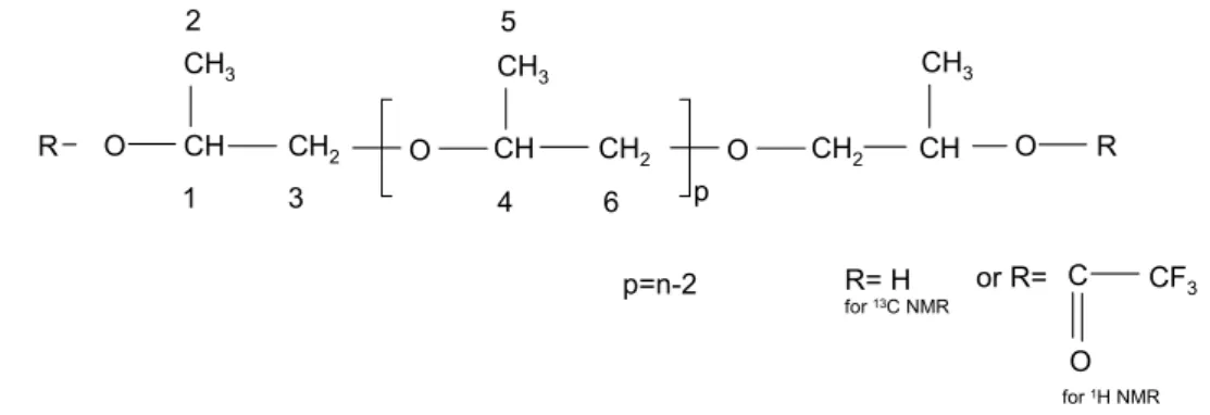
In practice, polyols are distinguished from short chain or low-molecular weight glycol chain extenders and crosslinkers such as ethylene glycol (EG), 1,4-butanediol (BDO), diethylene glycol (DEG), glycerine, and trimethylol propane (TMP). Polyols are polymers in their own. They are formed by base-catalyzed addition of propylene oxide (PO), ethylene oxide (EO) onto a hydroxyl or amine containing initiator, or by polyesterification of a di-acid, such as adipic acid, with glycols, such as ethylene glycol or dipropylene glycol (DPG). Polyols extended with PO or EO are polyether polyols (see Figure 1.1). Polyols formed by polyesterification are polyester polyols. The choice of initiator, extender, and molecular weight of the polyol greatly affect its physical state, and the physical properties of the polyurethane polymer. Important characteristics of polyols are their molecular backbone, initiator, molecular weight, percentage of primary hydroxyl groups, functionality, and viscosity.

Figure 1.1: Polyether Polyol.

1.1.1.2.2.- Polyisocyanates

A polyisocyanate is a molecule with two or more isocyanate functional groups R-(N=C=O)n ≥ 2. The isocyanates are very reactive components characterized by the presence

of the group –N=C=O. The rate of the reaction depends on the family of the isocyanate, the most important parameters being the amount of reactive groups and the functionality. The polyisocyanates are produced by the phosgenation of an amine. Molecules that contain two isocyanate groups are called diisocyanates, and molecules containing three isocyanate groups are called triisocyanates. There exist two main families of aromatic polyisocyanates: TDI

(22)

(toluene diisocyanate) and MDI (diphenylmethane diisocyanate) (see Figure 1.2). There exist also aliphatic polyisocyantaes, such as hexamethylene diisocyanate (HDI) or isophorone diisocyanate (IPDI).

(a) (b) Figure 1.2: Isomers of (a) TDI and (b) MDI.

The isocyanates present a double bond N=C which is quite polar and react with all the components having a mobile hydrogen. Depending on the kind of isocyanate, the charges can be presented in two mesomeric forms [Abder-Rahim 2001] (see Figure 1.3).

N N N R C O R C O R C O

..

⊕ ⊕

-..

N N N R C O R C O R C O

..

⊕ ⊕

-..

Figure 1.3: Mesomeric forms of isocyanate.

1.1.1.3.- Polycondensation of isocyanate-polyol to produce Polyurethane

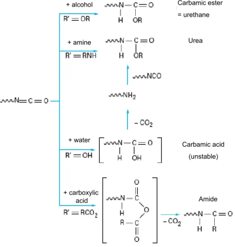
The polycondensation reaction is exothermic and consists of the chemical reaction of two molecules with different functional groups. For the polyurethane formation (polycondensate) it consists on the reaction of a hydroxyl group (-OH), the presence of a free “active” hydrogen and an isocyanate group (-NCO) (see Figure 1.4). The base of the chemistry of polyurethanes is the high reactivity of the isocyanates. Since the isocyanate group (-NCO) can react with alcohols, amines, carboxylic acids and water (see Figure 1.5), it can form bond of urethane, urea and amides. Reaction of an isocyanate with an alcohol yields a urethane, reaction of an isocyanate with an amine yields a urea, and reaction of an isocyanate with water results in intermediates which decompose to yield carbon dioxide and an amine, which further reacts to again form an urea. The reaction with water is used for the production of foams.

Polyurethanes are in the class of compounds called reaction polymer [Oertel 1985, Ulrich 1996, Woods 1990] and are formed by reacting a monomer containing at least two isocyanate functional groups with another monomer containing at least two alcohol groups, in the presence (or not) of a catalyst. To form a network a reaction either of a triol with a diisocyanate or of a triisocyanate with a diol is needed. The rate of the reaction varies as a function of the kind of alcohol used in the following order: primary alcohol > secondary alcohol > tertiary alcohol > phenol.

(23)

R N C O O

R' H

Figure 1.4: Polycondensation reaction: Polyurethane formation.

Carbamic ester = urethane Carbamic acid (unstable) Urea Amide + water + amine + alcohol + carboxylic acid Carbamic ester = urethane Carbamic acid (unstable) Urea Amide + water + amine + alcohol + carboxylic acid

Figure 1.5: Principal reactions with a polyisocyanate (taken from “techniques de l’ingenieur”). R’ represents each possible reactive functional group.

Though the properties of the polyurethane are determined mainly by the choice of the polyol, the isocyanate exerts some influence. The cure rate is influenced by the functional group reactivity and the number of functional isocyanate groups per reactive molecule. Polyurethanes are based upon a well-defined stoichiometry. The choice of isocyanate also

urethane function

(24)

aromatic isocyanates yellow with exposure to light, then the use of stabilizers may be included in the formulation; whereas those made with aliphatic isocyanates are stable [Randall 2002]. There are several kinds of polyurethanes: cellular, compacts, elastomers, coatings and adhesives. In this thesis we prepared polyurethane elastomers from polyether polyols and a trifunctional isocyanate.

1.1.1.3.1.- Secondary reactions

The urethane and urea groups already formed as presented in Figure 1.6, have other reactive hydrogen atoms that can react with another isocyanate giving as secondary products allophanates and biurets as presented in Figure 1.7.

Urea Urethane Allophanate Biuret Urea Urethane Allophanate Biuret

Figure 1.6: Secondary reactions of the isocyanate with urethane and urea groups (taken from “techniques de l’ingenieur”).

In the presence of certain “activators”, the isocyanates can react with each other and form by oligomerization, urediones (dimers), isocyanurates (trimers) or carbodiimides, as shown in Figure 1.7.

(25)

Isocyanurate Urediones Carbodiimide Isocyanurate Urediones Carbodiimide

Figure 1.7: Secondary reactions of oligomerization of the isocyanates (taken from “techniques de l’ingenieur”).

1.1.1.4.- Additives for polyurethanes’ preparation

The main additives used to produce polyurethanes are catalysts, chains extenders, surfactants, dyes, blowing agents, fillers, etc. The catalysts are accelerators of the reactions and for the polyurethane production they are used to reduce the curing times. There are two main catalysts used, the amines (i.e. Trietilendiamine or TEDA) and metallic salts (i.e. Dibutyldilaurate DBTL). In our case the catalyst was not used due to too fast reactions.

Polyurethanes made with aromatic isocyanates yellow with exposure to light, and the use of stabilizers may be included in the formulation (e.g. Irganox); whereas those made with aliphatic isocyanates are stable [Randall 2002].

1.1.2.- Model Networks

The rubbery networks prepared by random crosslinking of the precursor chains have inhomogeneous structures with a broad length distribution of the network strands; in addition, the characterization of the strand length distribution in elastomers is not possible by current analytical techniques. However end-linking end-reactive precursor chains of known molecular weight using multifunctional crosslinkers afford a tailor-made model network with a well characterized structure. In the case of complete reaction, the molecular mass of the network strands between neighboring crosslinks (Mc) is identical to that of the precursor chains, and

the junction functionality ( fe) is the same as the functionality of the crosslinker. To consider

the effect of the incomplete reaction on Mc and fe, the degree of the end-linking reaction (p) is

estimated from the amount of soluble species extracted after the reaction [Andrady et al. 1991, Urayama 2008].

An elastomer model network should have precursors with well known molecular weight and multifunctional crosslinker to be very close of the stoichimetric conditions, controlled lengths

(26)

of the network strands, reduced amount of trapped entanglements and inexistent or very few dangling chains [Urayama et al. 2009].

1.1.3.- Bimodal Networks

Experimentally, a bimodal network combines long- and short-polymer chains, presenting variable crosslinking density. Typically, bimodal networks result from blending difunctional long and short chains and crosslinking them together. They exhibit values of the modulus which increase very substantially at high elongations, thus giving unusually large values of the ultimate strength. This improvement in mechanical properties has been attributed to the limited extensibility of the short chains [Mark 1985, Mark and Erman 1988].

The theoretical analysis of bimodal networks, was first performed by Higgs and Ball [Higgs and Ball 1988]. These networks are composed of two types of chains, conveniently referred to as short and long chains, differing either in their molecular weight or in their chemical structure, thus obeying two distinct probability distribution functions for their end-to-end separations. The original theoretical approach, based on Gaussian phantom network chains for both components, was essentially developed for random bimodal networks with a random number of short or long chains connected at a given junction. Later, Kloczkowski et al. [Kloczkowski et al. 1991] considered the statistical mechanics of regular bimodal networks, which, by definition, have a fixed number Φs and ΦL of short and long chains, respectively, at

every junction and hence lend themselves to analytical solutions.

1.2.- Self-Assembled Monolayers (SAMs)

During several stages of sample preparation we prepared self-assembled monolayers (SAMs). The main goal of the SAMs preparation was to modify glass surfaces (glass lenses and glass plates) to bond the polyurethane to the glass in a covalent way (as presented in chapter 4). We also modified the surface of metallic molds with SAMs to make an easy release fluoro-terminated coating (also presented in chapter 4).

A self assembled monolayer (SAM) is an organized layer of amphiphilic molecules in which one end of the molecule, the “head group” shows a special affinity for a substrate (glass in our case); SAMs also consist of a tail with a functional group at the terminal end as seen in Figure 1.8 (b) and (c). The SAMs are created by the chemisorption of hydrophilic “head groups” onto a substrate from either the vapor or liquid phase [Schwartz 2001]followed by a slow two-dimensional organization of the “tail groups” (see Figure 1.8(a)) [Wnek and Bowlin 2004]. Initially, adsorbate molecules form either a disordered mass of molecules or form a “lying down phase” [Schwartz 2001], and over a period of hours, begin to form crystalline or semicrystalline structures on the substrate surface [Love et al. 2005, Vos et al. 2003]. The hydrophilic “head groups” assemble together on the substrate, while the tail groups (that can be hydrophilic or hydrophobic) assemble far from the substrate. Areas of close-packed molecules nucleate and grow until the surface of the substrate is covered in a single monolayer. Adsorbate molecules adsorb readily because they lower the surface energy of the

(27)

substrate [Love et al. 2005] and are stable due to the strong chemisorption of the “head groups.” These bonds create monolayers that are more stable than the physisorbed bonds of Langmuir-Blodgett films. The monolayer packs tightly due to van der Waals interactions, thereby reducing its own free energy [Love et al. 2005, Sullivan 2003, Oclin 2004]. Self-assembled monolayers (SAMs) offer a unique way to confine molecules in two dimensions. Figure 1.1 presents a schematic of self-assembled monolayers structures.

Anchoring group Head group Anchoring group Head group (a) (b) (c)

Figure 1.8: Schematic of SAM structure: (a) from solution to SAM; (b) schematic of head and functional group on the substrate, and (c) n-alkyl silane on glass.

1.3.- Rubber elasticity

In this section we present some fundamental concepts on the elasticity observed in elastomers also called rubber elasticity. These fundamentals are needed to better understand the physical and mechanical characterization of the polyurethane model networks presented in the next chapters.

Historically, the term rubber was used to refer to natural rubber only. The more modern term

elastomer is sometimes employed in relation to synthetic materials having rubber-like

properties, regardless of their chemical composition. The most important physical characteristic of the rubber-like state is a high degree of deformability exhibited under the action of relatively small stresses [Treloar 2005]. High extensibility and low Young’s modulus are the most remarkable properties of the rubber-like material; additionally, elastomers present particular thermal or thermoelastic properties. The thermoelastic effect

(28)

dates from Gough [Gough 1805] that made some experimental observations: 1) the elastomer in the stretched state, under a constant load, contracts (reversibly) on heating, and 2) the elastomer gives out heat (reversibly) when stretched. These observations were confirmed fifty years later by Joule [Joule 1859] who worked with perfectly reversible vulcanized rubber. The typical high elasticity of rubber arises from its molecular structure. Because the linear molecules are long and flexible, they take up random configurations under Brownian Thermal motions, like agitated snakes. When they are straightened out by an applied force, and released, they spring back to random shapes as fast as their thermal motion allows. In practice, the molecules are tied together by a few permanent chemical bonds, by a process known as “crosslinking”, to give the material a permanent shape. Thus, after crosslinking, rubber becomes a soft, highly elastic solid. Although rubber has a characteristic ability to undergo large elastic deformations, in practice many rubber springs are subjected only to relatively small strains, rarely exceeding 25% in extension or compression. A good approximation for the corresponding stresses is then given by conventional elastic analysis, assuming simple linear stress-strain relationships, because, like all solids, rubber behaves as a linearly elastic material at small strains. But some features of the behaviour of rubber can be understood only in terms of its response to large deformations. To treat large elastic deformations, we must consider how to characterize the elastic properties of highly extensible, nonlinearly elastic materials when a simple modulus of elasticity is not longer enough.

1.3.1.- Continuum Mechanics, Small and Large Strain Elasticity

Simple extension of an incompressible material such as rubber is defined by stretch ratios: λ1=λ, λ2=λ3=1/λ1/2 (Figure 1.9). This deformation satisfies the incompressibility condition

λ1λ2λ3=1.

x

z

Y

x

z

Y

Figure 1.9: Principal extension ratios in simple extension.

It is common to measure the stress in terms of the force f acting on a unit of undeformed cross-sectional area,

(29)

λ t

f = eq. 1.1

This equation is the large-deformation equivalent of a simple result: t=σ=Eε, applicable at small strains.

1.3.2.- Elastic properties at small strains

The elastic materials that are isotropic in their undeformed state can be described by two fundamental elastic constants. The first is related to the resistance to compression in volume under hydrostatic pressure called bulk modulus K, defined by:

⎟⎟ ⎠ ⎞ ⎜⎜ ⎝ ⎛ Δ = 0 V V K P eq.1.2

where P is the applied pressure and ΔV is the consequent shrinkage of the original volume V0.

The second constant describes the resistance to a simple shearing stress τ, called shear modulus G, defined by the relation:

γ τ =

G eq. 1.3

where γ is defined as the ratio of the lateral displacement d to the height h of the sheared material. The tensile modulus E (Young’s modulus of elasticity), defined by the ratio of a

simple tensile stress σ to the corresponding fractional tensile elongation ε, is given by:

G K KG E + = = 3 9 ε σ eq. 1.4 Figure 1.10 shows the schematic of the three main kinds of stress.

(30)

The Poisson’s ratio υ, defined as the ratio of lateral contraction strain ε2 to longitudinal

tension strain ε1 for a bar subjected to a simple tensile stress, is given by:

⎟⎟ ⎠ ⎞ ⎜⎜ ⎝ ⎛ + − = µ K µ K 3 2 3 2 1 υ eq. 1.5

For rubbers, Poisson’s ratio υ is close to one-half (typically, 0.4995) and the tensile Young’s modulus of elasticity is given almost by 3µ. If we consider rubber to be completely incompressible in bulk the υ=1/2 and the elastic behaviour at small strains can be described by a single elastic constant: µ [Gent 1992].

1.3.3.- The Strain Energy Function W

The finite strain deformation can be described by the deformation of a cube of unit dimensions in the undeformed state to the rectangular parallelepiped (see Figure 1.9), which has edges λ1, λ2, λ3 in the directions x, y, z, respectively In the deformed state the forces

acting on the faces are f1, f2, f3. The corresponding stress components as defined in the

deformed state are σxx, σyy, σzz where

1 1 3 2 1 _f f xx _λ _λ λ σ = = ₂ ₂ 1 3 2 _f f yy _λ _λ λ σ = = ₃ ₃ 2 1 3 _f f zz _λ_λ λ σ = = eq. 1.6 and these components of stress are different from those defined for small strain elasticity [Gent 1992]. The work done (per unit of initial undeformed volume) in an infinitesimal displacement from the deformation state where λ1, λ2, λ3 change to λ1+dλ1 , λ2 +dλ2, λ3+dλ3,

is 3 3 2 2 1 1dλ f dλ f dλ f dW = + + ₃ 3 2 2 1 1 λ λ σ λ λ σ λ λ σ d d d yy zz xx ₊ ₊ = eq. 1.7

For an elastic material the work done can be equated to a change in the stored elastic energy U=W. In the case of rubbers it is usual to consider a reversible isothermal change of state at constant volume, so that the work done can be equated to the change in the Helmholtz free energy A, i.e. ΔU=ΔA. Then W is called the strain energy function because it defines the energy stored as a result of the strain, i.e.

W=f(λ1, λ2, λ3) eq. 1.8

Because rubber is an isotropic material the form of this function f must be independent of the choice of the coordinates axes. For simplicity it should also become zero when denoted

(31)

λ1=λ2=λ3=1, i.e. for zero strain. A further requirement is that for small strain, we should

obtain Hooke’s law for simple tension. An equation which satisfies these requirements is

(

₁2 ₂2 ₃2 3

)

1 + + −

=C λ λ λ

W eq. 1.9

where C1 is half the shear modulus µ. To obtain a stress-strain relationship from this equation

it is invoked equation 1.10, together with the assumption that rubber is incompressible: λ1λ2λ3=1, and λ1=λ, λ2=λ3=1/λ1/2. Then equation 1.9 becomes

⎟ ⎠ ⎞ ⎜ ⎝ ⎛ ₊ ₋ = ₁ ₂ 2 3 λ λ C W eq. 1.10

and from 1.10 we have ⎟ ⎠ ⎞ ⎜ ⎝ ⎛ − = ∂ ∂ = 2 ₁ 1₂ λ λ λ C W f eq. 1.11

This equation is more usually represented as a consequence of the molecular theories of a rubber network. It follows from purely phenomenological considerations as a simple constitutive equation for the finite deformation of an isotropic, incompressible solid. Materials which obey this relationship are sometimes called neo-Hookean [Ward and Hadley 1998, Gent 1992].

1.3.4.- Strain Invariants

A general treatment of the stress-strain relations of rubber-like solids was developed by Rivlin [Rivlin in Eirich 1956], assuming only that the material is isotropic in elastic behaviour in the unstrained state, and incompressible in the bulk. Symmetry considerations suggest that appropriate measures of strain, independent of the choice of the axes, are given by three invariants, defined as:

2 3 2 2 2 1 3 2 1 2 3 2 3 2 2 2 2 2 1 2 2 3 2 2 2 1 1 λ λ λ λ λ λ λ λ λ λ λ λ = + + = + + = I I I eq. 1.12

Moreover, for an incompressible material I3 is identically unity; hence only two independent

measures of strain, namely I1 and I2, remain. It follows that the strain energy density W (i.e.,

the amount of energy stored elastically in unit volume of material under the state of strain specified by λ1, λ2, λ3 is a function of I1 and I2 only:

(32)

(

₁ −3, ₂ −3

)

=W I I

W eq. 1.13

(Since I1 and I2 take the value 3 when λ1 = λ2 = λ3 = 1, subtracting this amount gives strain

measures that go to zero in the undeformed state). Furthermore, because I₁− I3, ₂ −3 are of second order in the strains ε1, ε2, ε3, the strain energy function at sufficiently small strains

must take the form

(

₁ 3

)

₂

(

₂ 3

)

1 − + −

=C I C I

W eq. 1.14

where C1 and C2 are constants. This particular form of the strain energy function was

originally proposed by Mooney [Mooney 1940] and is often called Mooney-Rivlin equation.

1.3.5.- The statistical mechanical theory of rubber elasticity

1.3.5.1.- Statistical theory of rubber elasticity

Polymer networks are unique in their ability to reversibly deform several hundreds percent. This deformability arises from the entropic elasticity of the polymer chains. The early molecularly based statistical mechanical theory was developed by Wall [Wall 1942] and Flory and Rehner [Flory and Rehner 1943], with the simple assumption that chain segments of the network deform independently and on a microscopic scale in the same way as the whole sample (affine deformation). The simplest model that captures this idea is the affine network model originally proposed by Kuhn (see Figure 1.11). The main assumptions of the affine model are the following [Gedde 1999]: 1) the chain segments between crosslinking points can be represented by Gaussian chains; 2) the networks consist of N-chains per unit volume. The entropy of the system is the sum of the entropies of the individual chains; 3) the relative deformation of each network strand is the same as that on a macroscopic level i.e. the relative deformation imposed on the whole network is affine; then the crosslinks are assumed to be fixed in space at positions exactly defined by the specimen deformation ratio; 4) the unstressed network is isotropic; and 5) the volume remains constant during the deformation.

b l

Figure 1.11: Schematic representation of the equivalent chain of Kuhn. Assembly of ‘n’ rigid

rods with a fixed length ‘l’.

(33)

James and Guth [James and Guth 1943] avoiding the assumptions made in the affine model, treated a phantom network consisting of Gaussians chains having no material properties. In the phantom model, the ends of the network strands are joined at crosslinking functions that can fluctuate (are not fixed in the space as in the affine model). These two theories are in a sense ‘limiting cases’ with the affine network model giving an upper bound modulus and the phantom network model theory the lower bound. Figure 1.12 shows schematically the differences between the affine and phantom network model.

Figure 1.12: Schematic representation of the deformation of a network according to the affine

network model and the phantom network model. The unfilled circles indicate the position of the crosslinks assuming affine deformation (phantom network) [Taken from Gedde 1999]. The simplest way to describe a polymer chain is with the freely jointed chain model which assumes a polymer chain as a random walk and neglects interactions between monomers (see Figure 1.11). Because a long, flexible molecule can be represented to good approximation by a randomly arranged chain of ‘n’ freely joint links, each of length ‘l’, the distribution of the end-to-end lengths ‘r’ obeys a Gaussian probability function, at least for small end-to-end distances:

(

2 2

)

exp ) (r C r P = −β eq. 1.15

where the parameter β2_{is given by 3/2nl}2_{. The mean square distance between the ends for free}

chain (phantom chains) averaged over all configurations is denoted by < r2_>

0 and is given by

nl2 or 3/2β2_{. Then the distribution of end-to-end lengths ‘r’ is well represented by [Flory 1985,}

Gedde 1999]: ⎥ ⎥ ⎦ ⎤ ⎢ ⎢ ⎣ ⎡ ⎟ ⎟ ⎠ ⎞ ⎜ ⎜ ⎝ ⎛ − ⎟ ⎟ ⎠ ⎞ ⎜ ⎜ ⎝ ⎛ = 2 0 2 2 / 3 0 2 ₂ 3 exp 2 3 ) ( r r r r P π eq. 1.16

(34)

(

)

⎟⎟ ⎟ ⎠ ⎞ ⎜⎜ ⎜ ⎝ ⎛ ⎟ ⎟ ⎠ ⎞ ⎜ ⎜ ⎝ ⎛ − ⎟ ⎟ ⎠ ⎞ ⎜ ⎜ ⎝ ⎛ = = 0 2 2 0 2 ₂ 3 2 3 ln 2 3 ) ( ln r r r k r P k S

π

eq. 1.17

which after simplification becomes

⎟ ⎟ ⎠ ⎞ ⎜ ⎜ ⎝ ⎛ − = 0 2 2 2 3 r r k C S eq. 1.18 where C is a constant.

1.3.5.1.1- Affine network model

Figure 1.13 presents the sketch of a molecular strand in a network in the undeformed state (end-to-end vector r0=(x0,y0,z0)) and in the deformed state (end-to-end vector r=(x,y,z)). The

deformed and undeformed configurations are related through the stretch (λ1, λ2, λ3) by:

0

1x

x=λ y=λ₂y₀ z =λ₃z₀

Figure 1.13: Affine deformation of a single chain from the unstretched state r0=(x0,y0,z0) to

the stretched state r=( x0λ1, y0λ2, z0λ3).

Recalling the assumptions and definitions made above it is possible to compute the difference in entropy ΔS between n chains in the stretched and unstretched state. Each chain being composed of ‘N’ Kuhn monomers of length ‘l’ with end-to-end vector ‘r’, we have:

) 3 ( 2 1 2 3 2 2 2 1 + + − − = ΔS nk λ λ λ eq. 1.19

where k is the Boltzmann constant. Assuming that the main contribution to the free energy of the network comes from the changes in entropy the free energy required to deform a network is given by:

(35)

) 3 ( 2 2 3 2 2 2 1 + + − = Δ − =

ΔF_network T S_network nkT λ λ λ eq.1.20

If the number of chains n is now expressed per unit volume, the prefactor in equation 1.20 has the meaning of a shear modulus µ:

s M RT T k V nkT µ= =υ = ρ eq. 1.21

where, υ (=n/V=ρNav/ Ms) is the number of network strands per unit volume, ρ is the density,

Ms is the number-average molar mass of network strand, and R is the gas constant. The

network modulus increases linearly with the temperature because its origin is entropic, analogous to the pressure of an ideal gas. The modulus also increases linearly with the number density of network strands. The equation 1.24 states that the modulus of any network polymer is kT per strand. The affine predictions for the engineering stress in uniaxial deformation at constant network volume can be rewritten using the shear modulus [Rubinstein and Colby 2003]: ⎟ ⎠ ⎞ ⎜ ⎝ ⎛ ₋ = ₂ min 1 λ λ μ σ_no _al eq. 1.22

These classical stress-stretch equations are quite general, and the physics behind such classical models is the entropic elasticity of polymer chains.

1.3.5.1.2- Phantom network model

In this model, the ends of network strands are attached to other strands at crosslinks, which can fluctuate around their average position. These fluctuations lead to a net lowering of the free energy of the system by reducing the cumulative stretching of the network strands. The principal parameter of the phantom network is the functionality ‘f’ given by the number of segments between crosslinking points, which adds a corrective term to the shear modulus [Rubinstein and Colby 2003]:

⎟⎟ ⎠ ⎞ ⎜⎜ ⎝ ⎛ − = − = f M RT f f T k µ s 2 1 2 ρ υ eq.1.23

For any functionality f, the phantom network modulus is lower than the affine network modulus because allowing the crossslinks to fluctuate in space makes the network softer. The typical functionality of a network is 3 or 4. For f=3, the phantom prediction is one third of the affine network modulus. In the limit of high functionality f, the crosslinks in the phantom network do not fluctuate and are almost fixed in space as in the affine network model.

(36)

1.3.6.- Thermodynamics of elastomers deformation

To better understand the physics of the rubber elasticity it is important to separate the elastic force into entropic and energetic contributions. Stress acting on the rubber network will stretch out and orient the chains between the crosslink joints. This will decrease the entropy of the chains and hence give rise to an entropic force. The change in chain conformation is expected to change the intramolecular internal energy. The packing of the chains may also change affecting the intermolecular-related internal energy. Both the intra- and

intermolecular potentials contribute to the force. The following thermodynamic treatments yield expressions differentiating between the entropic and energetic contributions to the elastic force.

According to the first and second laws of thermodynamics, the internal energy change (dU) in a uniaxially stressed system exchanging heat (dQ) and deformation and pressure volume work (dW) reversibly is given by:

TdS dQ= eq. 1.24 fdL pdV dW =− + eq. 1.25 then, fdL pdV TdS dU = − + eq. 1.26

where dS is the differential change in entropy, p dV is the pressure volume work and f dL is the work done by deformation. The force is a vector (denoted f) but in this treatment is treated as a scalar (denoted f; being the absolute value of the vector). Because of the very small compressibility of elastomers P dV is much smaller than f dL under most circumstances, and we can approximate the work as f dL. The Helmholtz free energy F is defined as internal energy minus the product of the temperature and entropy:

TS U

F = − eq. 1.27

The change in the Helmontz free energy is a thermodynamics state function of variables T, V, and L: SdT TdS dU TS d dU dF = − ( )= − − = −SdT − pdV + fdL eq. 1.28 The change in Helmholtz free energy can be written as a complete differential:

(37)

dL L F dV V F dT T F dF V T L T L V, , , ⎟ ⎠ ⎞ ⎜ ⎝ ⎛ ∂ ∂ + ⎟ ⎠ ⎞ ⎜ ⎝ ⎛ ∂ ∂ + ⎟ ⎠ ⎞ ⎜ ⎝ ⎛ ∂ ∂ = eq.1.29

Combining equation 1.29 with 1.30, we identify the partial derivatives of the Helmholtz free energy: S T F L V − = ⎟ ⎠ ⎞ ⎜ ⎝ ⎛ ∂ ∂ , eq. 1.30 p V F L T − = ⎟ ⎠ ⎞ ⎜ ⎝ ⎛ ∂ ∂ , eq. 1.31 f L F V T = ⎟ ⎠ ⎞ ⎜ ⎝ ⎛ ∂ ∂ , eq. 1.32

The force applied to deform a network consists then of two contributions:

S E L V V T V T f f T f T L U f L F ₌ ₊ ⎟ ⎠ ⎞ ⎜ ⎝ ⎛ ∂ ∂ + ⎟ ⎠ ⎞ ⎜ ⎝ ⎛ ∂ ∂ = = ⎟ ⎠ ⎞ ⎜ ⎝ ⎛ ∂ ∂ , , , eq. 1.33

where fE is the energetic contribution to the force, related to the change in internal energy

with sample length, and fS is the entropic term, product of the temperature and the change in

entropy with sample length. In ‘ideal networks’ there is no energetic contribution to the elasticity, so fE =0 [Treloar 2005, Gedde 1999, Rubinstein and Colby 2003].

1.3.7.- Deviations from rubber elasticity theory

Both affine and phantom network models predict the same dependence of stress on deformation. However, a comparison of the classical forms with experiments indicates two major disagreements (see Figure 1.14). Experiments demonstrate softening at intermediate deformations and hardening at higher deformations. In unfilled rubbers the softening indicates the presence of entanglements in addition to crosslinks, while in filled rubbers it is typically due to the breakup of interactions between fillers. The strain hardening at high deformations can be explained by the non-Gaussian statistic of strongly deformed chains. The finite extensibility is the major reason for strain hardening at high elongations.

(38)

Figure 1.14: Engineering stress in tension for a crosslinked rubber. The solid line the classical nominal stress fit to small strain data [taken from Treloar 2005].

1.3.7.1.- Chain entanglements

In the affine network model strands are fixed in space, and in the phantom network model strands are allowed to fluctuate around some fixed position in space. In both models, chains are only aware that they are strands of a network because their ends are constrained by crosslinks. In real networks, the chains impose topological constraints on each other because they can not cross, and these topological constraints are called entanglements. The surrounding chains on a given strand is represented in the Edwards tube model by a quadratic constraining potential acting on every monomer of each network strand; in this model fluctuations driven by the thermal energy kT are allowed. The tube diameter a can be interpreted as the end-to-end distance of an entanglement strand of Ne monomers (a=bNe1/2)

where b is the Kuhn segment length. The strand between entanglement has an average molar mass Me= Ne M0. For a purely entangled system, Me substitutes the average molecular weight between network strands in the determination of the modulus [Rubinstein and Colby 2003]:

e e

M RT

µ = ρ eq. 1.34

The small strain modulus of an entangled and crosslinked polymer network can be approximated by: ⎟⎟ ⎠ ⎞ ⎜⎜ ⎝ ⎛ + ≈ + ≅ e x e x M M RT µ µ µ ρ 1 1 eq. 1.35

Then, the modulus is controlled by crosslinks for low molar mass strands between crosslinks (µ~µx for Mx<Me) and by entanglements for high molar mass (µ~µe for Mx>Me).

As the material is being stretched the entanglements (unlike the fixed chemical crosslinks) can slip and effectively reorient strands in the tensile direction resulting in a reduction of the

strain hardening

(39)

apparent modulus and hence a softening observed relatively to an unentangled network with an identical small strain modulus. Several molecularly based models have been proposed to account for the presence of entanglements in the network and a good review can be found in [Rubinstein and Panyukov 2002].

A detailed comparison between models and experimental data would go beyond the purpose of this thesis. Rubinstein and Panyukov proposed however a particularly simple expression for the engineering stress as a function of λ based on a so-called slip-link model which introduces a confining potential around the chains. Their prediction for uniaxial deformation is given by: ⎟ ⎠ ⎞ ⎜ ⎝ ⎛ − = − 2 1 * 1 ) ( λ λ σ λ f eq. 1.36

where )_f*(_λ−1 _{is the prediction of the Mooney ratio on the nonaffine tube model.}

Figure 1.15 shows a comparison of cross-linked PDMS with the Mooney-Rivlin expression, nonaffine tube model, and the sliptube model.

Figure 1.15: Comparison of cross-linked PDMS (open circles) with the Mooney-Rivlin

expression (dotted line), nonaffine tube model (dash-dotted line), and the sliptube model (solid line) (taken from Rubinstein and Panyukov 2002).

1.3.7.2.- Finite extensibility

The assumption of Gaussian chain statistics does not predict any finite extensibility of polymer chains. At high strains, polymer chains are not organized as random coils and orient

Fracture by cavitation of model polyurethane elastomers

HAL Id: pastel-00578499

https://pastel.archives-ouvertes.fr/pastel-00578499

Fracture by cavitation of model polyurethane elastomers

Antonella Cristiano

To cite this version:

THESE DE DOCTORAT DE

L’UNIVERSITÉ PIERRE ET MARIE CURIE

Mme. Antonella CRISTIANO

DOCTEUR de l’UNIVERSITÉ PIERRE ET MARIE CURIE

FRACTURE BY CAVITATION OF MODEL

POLYURETHANE ELASTOMERS

Acknowledgments

Table of Contents

General Introduction

Chapter 1

Introduction

1.1.- The Networks

..

..

..

..

..

..

..

..

..

..

-..

..

..

..

..

..

..

..

..

..

..

-..

1.2.- Self-Assembled Monolayers (SAMs)

1.3.- Rubber elasticity

x

z

Y

x

z

Y

(

)

(

)

(

)

(

)

(

)

(

)

π