Why are there so many long-term unemployed in Paris?

HAL Id: halshs-01102753

https://halshs.archives-ouvertes.fr/halshs-01102753

Preprint submitted on 13 Jan 2015

HAL is a multi-disciplinary open access archive for the deposit and dissemination of sci-entific research documents, whether they are pub-lished or not. The documents may come from teaching and research institutions in France or abroad, or from public or private research centers.

L’archive ouverte pluridisciplinaire HAL, est destinée au dépôt et à la diffusion de documents scientifiques de niveau recherche, publiés ou non, émanant des établissements d’enseignement et de recherche français ou étrangers, des laboratoires publics ou privés.

Why are there so many long-term unemployed in Paris?

Florent Sari, Yannick l’Horty

To cite this version:

Florent Sari, Yannick l’Horty. Why are there so many long-term unemployed in Paris?. 2015. �halshs-01102753�

WORKING PAPER

N° 2015 - 1

Why are there so many long-term unemployed

in Paris?

Y

ANNICK

L’H

ORTY AND

F

LORENT

S

ARI

www.tepp.eu

TEPP - Institute for Labor Studies and Public Policies

Why are there so many long-term

unemployed in Paris?

Y

L’H

*

F

S

**

*Université Paris-Est, ERUDITE, UPEC, UPEM and TEPP-CNRS, 5 bd Descartes, 77454 Marne-la-Vallée Cedex2. Email [email protected]

** Université de Nantes, LEMNA and TEPP-CNRS, Chemin de la Censive du Tertre, 44322 Nantes Cedex3. Email [email protected]

Parisian jobseekers present an abnormally high risk of long-term unemployment, all things being equal. It is a phenomenon specific to Paris and districts closest to the centre. This is a paradox in a job market particularly dense and active. In this article, we propose an explanation which combines the essentials of two mechanisms, Skill Mismatch and Spatial Mismatch. It is because Parisian jobseekers are geographically far from the jobs that suit their profiles that they present a high risk of long-term unemployment. This explanation is corroborated by a model of spatial regimes and correlated errors on the Ile-de-France data and local durations of unemployment.

Key words : Paris, unemployment, spatial econometrics, spatial regime models, Skill Mismatch, Spatial Mismatch.

I

The fact is surprising yet well-established: Parisians are amongst the French the most exposed to the risk of long-term unemployment. We count 90,000 jobsekers of more than a year, 47.6 % of the jobseekers compared to 42.3 % for Ile-de-France and 43.3 % for the whole of metropolitan France. These figures from mid-2014 make Paris the 7th highest French department in terms of duration of unemployment1. However, the relative situation of Paris has improved since the crisis. At the end of 2008, Paris was the department of metropolitan France with the highest percentage of jobseekers of more than a year. Figure 1 presents this statistic, calculated monthly by Pôle Emploi, for each department of Ile-de-France, for the entire region and for the whole of France during the period 1996-2014. The permanance of this Parisian particularity is clear. The percentage of jobseekers of more than a year is always higer in Paris during the period. The difference between the percentage of long-term jobseekers in Paris and in Ile-de-France peaks at the end of 2008 at 9 percentage points. It is only 5.4 points in mid-2014, which is nevertheless high.

Figure 1. Percentage of long-term jobseekers among total jobseekers

Field: Jobseekers registered at the end of the month with Pôle Emploi and registered for more than a year in

categories A, B, C, as a total of jobseekers, by region and by department.

Source : STMT - Pôle Emploi, DARES.

1 _{After Aisne, the Vosges, Allier, Pas-de-Calais, Eure, the Somme and the Nord are historically the industrial}

How can we explain this paradox? How can such an active, dense job market go hand-in-hand with such a feeble rate of return to employment? To answer these questions, we solicit the hypotheses from urban economics and labour economics, according to which the location of individuals and the spatial organisation of towns could complicate a return-to-work. We use two principal mechanisms. On one side, we have the disadvantageous effect of the physical disconnection between the place of residence and the centres of work (the hypothesis of Spatial Mismatch proposed by KAIN in 1968) and, on the other side, local skills mismatch in terms of jobs on offer and jobs sought (the hypothesis of Skill Mismatch), whose first proponents for the labour market were without doubt JACKMAN et al. (1990). Taken separately, these explanations do not appear necessarily convincing. A priori there is no problem of physical distance from employment for Parisians, given that its inner suburbs appear rich in jobs. The diversity of jobs on offer also seems to go against the idea of a skill mismatch at a local level. But considered together, these explanations become pertinent. Unemployed Parisians live close to a large source of jobs, but their characteristics do not correspond to jobs sought. This is the hypothesis that we want to verify in this work.

This study follows previous work using applied microeconomics to better analyse the geography of unemployment in France (BOUABDALLAH et al., 2002; GASCHET and GAUSSIER, 2004; DUGUET et al., 2009) and particularly follows studies specific to Ile-de-France (GOBILLON and SELOD, 2007; DUGUET et al., 2009; KORSU and WENGLENSKI, 2010; GOBILLON et al., 2011). Compared to all these works, the originality of ours is to focus on the question of the Paris singularity, which has not been explicitly investigated by any previous study, and to attempt to validate an explanation using a specific model.

Firstly, we offer a brief literature review – theoretical and empirical- in order to understand the potential links between spatial organization of a territory and unemployment-to-work

transitions. Secondly, we use an exhaustive administrative source, the Pôle Emploi files, to construct fairly precise spatiale flow indicators to describe the return-to-work and to give us an original overview of the Paris situation. Finally, we verify empirically our hypotheses with the help of a spatial econometrics model.

E

P

To interpret the overexposure of Parisians to long-term unemployment, we favour two hypotheses inspired by urban economics and labour economics. The first is Spatial Mismatch, proposed initially by KAIN (1968) which explains local unemployment by the physical distance of jobs. The second is Skill Mismatch, which focuses on the local imbalance between jobs on offer and jobs demanded. The first theoricians of the labour market were undoubtedly JACKMAN et al. (1990). We develop each hypothesis.

The Spatial Mismatch hypothesis

In a 1968 article, Kain advances the idea whereby living in locations far from jobs has important consequences on unemployment2. This intuition led to the emergence of a vast body of literature in the United States focused on the possible relationships between the urban organisation of towns and the local labour market. Together, this literature identifies two principal mechanisms that link this hypothesis to situations experienced in the labour market by certain residents (ARNOTT, 1998).

The first mechanism is the cost of travel. A physical disconnection between the place of residence and the place of work could lead to high travel costs because certain localities are not well-served by public transport. These costs might be aggravated by problems of traffic congestion or by poor public transport, a phenomenon encountered in the Paris region. In this

2 _{Initially, KAIN’s studies on this hypothesis aimed at explaining the differences in employment or}

unemployment rate between Blacks and Whites in the United States. More generally, this hypothesis concerns particular population categories considered disadvantaged in the labour market. In this study, we do not make distinctions by sub-populations. We suppose that this problem could concern all residents.

context, jobseekers residing in towns disconnected from employment centres are confronted by monetary and time costs often too high in relation to the wages offered (COULSON et al., 2001; BRUECKNER and ZENOU, 2003). The second mechanism comes from the differents characteristics of the job search process. Firstly, an individual living far from employment centres could encounter difficulties in obtaining information on available work (ROGERS, 1997). IHLANFELDT and SJOQUIST (1990, 1991) show that the physical distance from employment tends to reduce the available information on job vacancies. In these conditions, seeking work far from the domicile could prove too expensive. Individuals will look for a suitable job in a relatively restricted zone, close to home, and will do so even if these jobs are of poor quality (DAVIS and HUFF, 1972).

Some empirical studies have tested this hypothesis for France. BOUABDALLAH et al. (2002) were among the first to confirm this hypothesis by showing that the widening of the zone of jobseeking leads to a reduction in the duration of unemployment. The resulting increase in job offers compensates for the increased costs of prospection linked to the widening of area. In line with previous work, CAVACO and LESUEUR (2004) highlight the particularly discriminating effect of spatial contraints (such as the distancing of zones of concentration of employment or job agencies) during their research into episodes of unemployment. GASCHET and GAUSSIER (2004) also confirm the negative effects of poor accessibility to work on the duration of unemployment in the Bordeaux metropolitan area. DETANG-DESSENDRE and GAIGNÉ (2009) show that better accessibility increases the probability of finding work for the residents of urban and rural fringe zones. RUPERT et al. (2009) show that for a given wage, workers are less likely to accept job offers far from their places of residence.

For the Paris region, GOBILLON and SELOD (2007) are among the pioneers. They highlight the relationship between physical accessibility to employment and return-to-work. DUGUET

et al. (2009) also find that a poor access to employment can increase the duration of unemployment and decrease the rate of exit from unemployment. More recently, KORSU and WENGLENSKI (2010) and GOBILLON et al. (2011) also show that limited accessibility significantly increases the risk of unemployment (notably long-term unemployment) for the residents of the region.

The Skill Mismatch hypothesis

The other hypothesis that we employ is that of Skill Mismatch. It is based upon the theory by which, locally, some individuals do not have the skills and qualifications necessary to apply for available job vacancies. This results in difficulties finding a job and, where they do find work, it is generally of poor quality and low-paid (PASTOR and MARCELLI, 2000). We then talk about a mismatch between the skills expectations of employers and the qualifications of jobseekers (CARLSON and THEODORE, 1995; DANZIGER and HOLZER, 1997 ; GORDON,2002).

Numerous empirical studies seem to confirm this hypothesis. For the United States, BAUDER and PERLE (1999) confirm that Blacks are disadvantaged in a context where the labour market requires higher skills but they suffer from a low level of education. MANACORDA and PETRONGOLO (1999) particularly confirm this hypothesis. The authors find that the Skill Mismatch is not a serious problem in the labour markets of OECD countries, except for less qualified workers in Great Britain. However, their work does not permit a very precise analysis of the Skill Mismatch at town or neighbourhood level. We could also cite the theoretical model developed by THISSE and ZENOU (2000) in which the authors explore the interactions between heterogeneous workers and firms with differing demands for skill levels. In an imperfect market, they find that unemployment could be attributed to an imbalance between the offer and demand for skills. STOLL (2005) also verifies this hypothesis for the suburbs of Los Angeles and Atlanta. He finds a negative relation between poor matching of

measured skills and the local level of employment. This mismatch is at the origin of nearly a third of the differences in observed employment rates between Blacks and Whites. Finally, HOUSTON (2005) innovates by simultaneously considering the Skill Mismatch and Spatial Mismatch Problems. He shows with the help of a conceptual model that each cannot be considered separately. On the contrary, they can be mutually reinforcing and in fine explain differences in unemployment observed within metropolitan areas. By combining these two hypotheses we can find a plausible explanation that can be tested with the data. The intuition is simple: Parisian jobseekers live close to a large source of employment but the characteristics of the jobs on offer are not those of the jobs sought. In addition, the job offers that correspond to the characteristics of the jobseekers are, generally, physically far from the centre of Paris. Given the profile of Paris jobseekers, there are suitable job offers but they are situated in the middle suburbs of the Paris metropolitan area, far from the city centre. Physically distanced from job offers that suit them, Parisian jobseekers experience a longer jobsearch than jobseekers in other towns and departments.

M

Comparisons of the unemployment rate are based on stock indicators that are informative but inadequate for a complete diagnosis of the nature and causes of the problem. They need to be complemented by labour market flow indicators, such as the rate of unemployment entry and exit, and the duration of unemployment.These flow indicators pose a problem of definition and observation. To calculate them, the best source is the historical statistics records (FHS) of Pôle Emploi, a government source. This permits us to follow the individual paths of jobseekers by recording each successive step from their first registration with their Job center, but it does not follow jobseekers after they are hired if they are no longer registered.

We use the indicators calculated by DUGUET et al. (2009) in Ile-de-France and in 22 metropolitan regions3. To be able to follow jobseekers over a long enough period, we limit ourselves to the group of persons who registered between July 1, 2001 and June 30, 2002. July 1 is chosen because it coincides with the implementation of a new system of unemployment insurance. Therefore we study a homogeneous period in terms of benefits. The record used is a version of FHS updated on March 31, 2006. Therefore, we study this cohort of unemployed over a period of nearly five years.

To model the unemployment duration, we use a Weibull specification where the rate of exit from unemployment is a function of time spent in unemployment as well as local fixed effects and also depends on the characteristics of the individual, such as age, sex, or level of education. The use of administrative records poses the question of measuring the exit from unemployment. By crossing two definitions of exit from unemployment, removal from the lists and declared return-to-work, and two measures of the sustainability of the exits, from at least one month and six months and more, we obtain four definitions for exit from unemployment. The choice of one or another of these definitions influences the number of exits. By limiting the observation to declared return to work, the number of exits is far lower. In Ile-de-France, it is halved (308,619 rather than 629,046). By limiting ourselves to sustainable exits, we reduce the number of exits by about a quarter (we count 258,952 exits of six months and more with declared return to work). Annex A presents the results of estimations for the Ile-de-France region.

Our dependent variable is this local unemployment duration calculated from individual data. One might suspect an endogeneity problem with other socio-demographic indicators since it seems difficult to distinguish whether an individual is unemployed because he or she lives in a particular town or if he or she lives in a particular town because they are unemployed. This

3 _{The work of Duguet et al. (2009) also proposes a detailed explanation of the econometircs methodology used to}

problem is limited in our case because i) the residential mobility is rare in France, especially for job seekers; ii) we follow a cohort of new jobseekers who were previously employed and iii) we control for the characteristics of these job seekers. Most importantly, we want to explain excessive unemployment duration within Paris which is not a deprived location.

Stylised facts: the disadvantage of Paris

Table 1 shows the disadvantage of the Paris labor market regarding the exit rate of unemployment. If the comparison of unemployment rates in the first quarter 2014, between the Ile-de-France and metropolitan France, seems to be favorable to the first (the unemployment rate is 8.6% against 9.7%), it is no longer the case when one is interested in unemployment durations disparities. Indeed, the Ile-de-France has the highest unemployment durations comparatively to the rest of France. This is true for both the definitions used (removal from the lists and declared return-to-work). Unemployment durations before a removal from the lists and declared return-to-work are 11.4 months against 10.3 months and 51.4 months against 40.4 months, respectively. Paris is one of the French departments where job seekers have, on average, the least chance of leaving unemployment. The odds are much lower than the French average (10.5 months) and they are also relatively to any department of Ile-de-France. The average length enrollment to job center is more than 13 months in Paris, against 11 months in the departments of the region, and 9.3 months in Essonne.

Table 1. Unemployment in Ile-de-France

Rate of unemployment (2014) Duration of unemployment gross net Obs. Removal from lists Return to work Removal from lists Return to work Metropolitan France 36 566 9,7% 10,5 31,1 10,2 30

Metro France (outside

IdF) 35 266 9,8% 10,3 28,9 10,3 28,9

Ile-de-France 1 300 8,6% 11,4 40,4 10,1 34,5

Seine et Marne (77) 514 7,9% 10,8 30,6 9,9 27,3 Yvelines (78) 262 7,1% 11 32 9 29,2 Essonne (91) 196 7,4% 9,3 28,4 8,5 25,7 Hauts-de-Seine (92) 36 7,6% 11,3 37,5 10,2 34,9 Seine-Saint-Denis (93) 40 12,7% 10,9 46,8 10,2 39,2 Val-de-Marne (94) 47 8,6% 10,8 37 9,9 31,9 Val-d'Oise (95) 185 9,8% 11 38,1 10,1 33,6

Source :INSEE, from historical statistical records of Pôle Emploi.

Notes: The averages are the averages weighted by the number of unemployed in the towns.

We also want to check if the problem is general, or if it particularly affects certain categories of jobseekers. For example, with Paris, the over-representation of occasional workers in the entertainment industry is sometimes cited as a reason for the high rate of unemployment. To check, we estimate two total rates of local exit, without or with control by individual jobseekers’ characteristics.4 If Paris jobseekers had the same socio-demographic profile of those of Ile-de-France, they would exit unemployment less quickly. This is linked to the fact that Paris jobseekers are more highly qualified than others, which have a favourable effect of the chances of exiting unemployment.

We compute the rate of survival of unemployment with the help of Kaplan Meier non-parametric estimates. The indicators obtained allow us to show descriptively the importance of locality to the duration of unemployment (another way of rendering the rate of exit from unemployment).

Figure 2 shows the distribution functions calculated for three classes of distance of towns from the centre of the region. The 10% of towns the closest to the centre (within a radius of 13 kilometres) are those where the durations of unemployment are highest, when one considers the definition “Removal from lists”. The 50% of towns the furthest from the centre (more than 39 kilometres) also have serious difficulties in terms of exit from unemployment. Beyond a duration of unemployment of 10 months, the two lines cross. This signifies that long-term jobseekers are more strongly represented in both towns closest to the centre and

4 _{These variables are sex, age, nationality, marital situation, number of children, highest educational qualification}

obtained, disability, type of work contract sought, trade (ROME code), reason for entering unemployment, RMI situation.

further from the centre. The 40% of towns within a radius of 13 and 39 kilometres are those where the durations of unemployment observed are the lowest of the groups. We will use these three statiscal classes in order to define our spatial regimes in the estimations.

Note that these inequalities cannot be explained by possible disparities in the socio-economic composition of jobseekers because our analysis of the net durations neutralises these effects. Highlighting a possible problem of physical distance from employment opportunities is not necessarily satisfactory since the highest durations are observed for the towns closest to the centre. Other factors must be identified to permit us to explain this particular pattern.

Figure 2. Net durations of unemployment and distance from centre

Reading: The threshold “ < 13 km” includes all the towns within a radius of 13 kilometres from the

centre of Paris (10 % of the towns). The threshold “ > 39 km” includes all the towns beyond a radius of 39 kilometres from the centre (50 % of the towns). The threshold “> 13 km &< 39 km” includes all the towns between the two distances (40 % of the towns). The distances are Euclidean.

Source: Historical statistical records of Pôle Emploi.

The spatial auto-correlation issue

The local duration of unemployment constitutes our variable of interest and we are concerned with its spatial auto-correlation. We calculate the Moran auto-correlation coefficient I for the

durations of unemployment, which could be interpreted as the relation of the covariance between contiguous observations and the total variance observed in the sample (Jayet, 1993). It is given by:

= ∑ ∑ ∑ ∑ ∑ ( − ̅)²( − ̅)( − ̅)

Where is a weighting which permits us to take into account the geographical proximity of spatial units i and j.

When I > I = (n − 1) I (respectively I < E[I]), the values taken by the durations are not placed randomly but are close (respectively distanced) for two neighbouring spatial units. The geographically close spatial units are also statistically close (respectively distanced) and we conclude the presence of a positive spatial auto-correlation (respectively negative). When I is close to E[I], we conclude the absence of spatial auto-correlation. In this case, we can establish no link between the statistical proximity and the geographical proximity of spatial units.

In fact, the calculation of the Moran index I is sensitive to the definition of the matrix of spatial weighting W( ). There are effectively several criteria to determine the spatial units that will be considered as neighbours: contiguity5, closest neighbours, distance. Given the clusters of homogeneous towns, we choose to construct a contiguity matrix, where the towns have links with their immediate neighbours. We present in Table 2 the auto-correlation coefficients (Moran I) of the net durations of unemployment obtained for different types spatially weighted matrices.

Table 2. Global spatial auto-correlation of duration of unemployment

Matrix W Moran I Distance-type p-value Queen 1 0,5101 0,0193 0,001 Queen 2 0,3295 0,0133 0,001 Queen 3 0,1954 0,0111 0,001 5

Distance < 6 km 0,4908 0,016 0,001

Source : Historical statistical records of Pôle Emploi. Notes : E[I] = -0,0009.

Whatever the type of matrix used, we see that the duration of unemployment presents a significant positive spatial auto-correlation that is relatively high. Then, the geographically neighbouring towns are also neighbours in terms of duration of unemployment. To consider the spatial auto-correlation problem in our data, we must use an appropriate model. We use the matrix of congituity of the type Queen to the order 1 because this presents the highest value for spatial auto-correlation.

Skill and Spatial mismatch indicators

To construct the others variables, we use two different sources of data. Firstly, we use census data produced by INSEE dating from 1999, because it is before the period covered by our Pôle Emploi data. Secondly, we use the Déclarations Annuelles de Données Sociales- annual declaration of workplace data (DADS)6, an exhaustive source of information on companies and their employees. Our DADS database contains 346,545 firms in Ile-de-France between 2002 and 2005, including 86,342 questioned on the four dates of the survey. They are part of 1149 towns in the region.

To test the Spatial Mismatch hypothesis, we use two different indicators. On one hand, we compute the Euclidean distance between the town of the residence and the centre of Paris. Even if towns such as Roissy, Cergy or Saint-Quentin attract more and more workers, Paris remains the most important centre of employment in Ile-de-France and so we consider it as the sole reference. On the other hand, we use an indicator on the density of accessible employment within a radius of 20 km from the centroid of the towns:

6

=_∑∑

Where is the density of jobs calculated for the town i, E is total jobs, PA is the total workforce, j is the total towns within 20 kilometres of a given town i.

To measure the Skill mismatch, we adapt the indicator of Jackman et al. (1990) that measures the difference between the relative proportions of unemployed by qualification according to the town. This indicator is theoretically interpretted by these authors as the share of structural unemployment having problems of skill mismatch. It corresponds to the semi-variance of the ratio between the rate of unemployment by skills (manual workers, employees, intermediate professions, and managers) and the total rate of unemployment (u) within the town:

= 1_{2 ! " with 0)} ) 1

A high value for this indicator means that some populations encounter more problems of unemployment than others, which shows that locally the jobs do not necessarily meet the needs of local populations and that mismatch explains an important part of local unemployment.

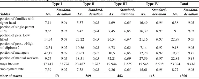
We include also control variables to account for differences in duration of unemployment observed between the towns of the region. Firstly, to control for potential differences in the socio-economic composition between towns, we construct a typology of towns from a principal component analysis then from an ascending hierarchical classification (Ward criteria). These methods are based upon the variables of the 1999 census which measures the proportion of each socio-professional category, the relative distribution of education degrees, as well as the proportion of single-parent families and foreigners residing in each town. The classification allows the creation of four groups of towns that are relatively homogeneous in

population: towns with a majority of the population highly qualified, populated essentially by managers (type I), towns with qualified populations with a proportion of single-parent families and foreigners above the average (type II), towns where the majority of residents are manual workers with low educational qualifications (type III), and towns where the proportion of manual workers, single-parent families and foreigners is high (type IV).

In addition to the location of existing jobs, those of jobs created or disappeared are equally important to explore the hypothesis of Spatial Mismatch. The towns that are dynamic in terms of creating or destroying jobs are those where the unemployed are more likely to experience short-term unemployment, because the turn-over is to the advantage of jobseekers. To measure the creation and destruction of jobs, we use annual employment flow indicators inspired by DAVIS and HALTIWANGER (1990), created from DADS. The gross creations of jobs correspond to the positive variations between employees N on two successive dates, and the gross destruction of jobs to negative variations. The volume of gross creation of employment *_+, in the town i between the dates t-1 and t is:

*+, = - ∆/0+, 0∈23

where *4 is the sub-total of companies e of the towns i for which the number of jobs at the end of the period is more than the number of jobs at the beginning of the period of observation, and ∆ operates the difference between t-1 et t. Similarly, the volume of gross destruction of jobs _+, is:

+, = - |∆/0+,| 0∈26

where * is the sub-total of companies e of the towns i that experience a negative variation in employment during the year.

In Table 3, we present some statistics on the indicators used for our analysis in taking into account the different spatial regimes used previously. Firstly, we come back to fact already highlighted by Figure 2: the net duration of unemployment varies strongly depending on locality and notably on the distance from the centre of Paris. The Parisian arrondissements (central city districts) as well as the closest suburbs are effectively those which record the longest net durations of unemployment, with an average duration of around 11.2 months. Conversely, the most favourable towns are those situated the furthest but not on the fringe of the region.

On average, the towns are located at 40 kilometres from the centre, but almost half of the sample is at more than 39 kilometres. We could suspect that these towns suffer from a particularly poor accessibility to jobs, according to the idea that jobs are mostly concentrated in the centre. Actually, the density of employment varies strongly according to the distance from the centre. The indicator is less than one in proximity to Paris because of the concentration of population and so its density is very high. For the year 2007, Paris and its inner ring counted more than 6,500,000 inhabitants (56% of the total population of the region), whereas the land area is 762 km² against more than 12,000 km² for the whole of the region (about 6%). On the other hand, the ratio is higher than one for the towns at a good distance from the centre, which is beyond 13 kilometres. This means that the competition within the labour force to find a job is possibly less strong. At the same time, the indicator does not allow us to know if it is high because of a large reservoir of jobs or a low level of workforce, which does not give us the same reality.

Table 3. Indicators according to locality

Distance to centre Variables Ile-de-France < 13 km 13 km >&< 39 km > 39 km

months)

1,285 0,788 1,292 1,215 Spatial Mismatch

Distance to centre (in km) 40,291 8,19 26,749 57,719

21,006 3,313 7,459 13,26

Job density (radius : 20 km) 1,406 0,951 1,265 1,588

0,298 0,079 0,259 0,212 Skill Mismatch

JLS Index 0,018 0,011 0,015 0,021

0,014 0,007 0,013 0,014

Skill Mismatch for NQ 0,134 0,139 0,118 0,145

0,054 0,063 0,05 0,052 Local dynamisme

Creation rate (standardised) 1,027 1,537 0,993 0,521

4,727 2,121 1,953 1,299

Destruction rate (standardised) 1,089 1,873 1,089 0,62

3,635 2,645 2,633 1,193

Observations 1 075 110 429 536

Sources Pôle emploi FHS, DADS 2002-2005, population census 1999 (INSEE).

Notes: The differences types are presented in italics. The statistics concern the 1075 towns for which the

duration of unemployment could be calculated.

The JLS indicator takes a higher value for the towns far from the centre. This may be a first indication of a mismatch of skills for some categories in these towns. The measure of the difference between the rate of people without degrees and local unqualified employment dynamism in the towns reveals a logic that is little different. The indicator is higher for the towns in the centre and those that are relatively far. The difference is lower for the towns at a middle distance, which tends to show that the situation there is more favourable for the unqualified.

Finally, we observe that the dynamism of the towns is strongly linked to their proximity to the centre of the region. The rates of creation and destruction (standardised) are the highest in the centre and the lowest in the furthest towns. The relatively high values for these two indicators show large movements of manpower and so a higher turn-over. Therefore, we can suppose that the weak dynamism for the towns most at the fringe could be a brake on a rapid exit from unemployment.

All these facts show the value of “cutting up” the country. It is highly probable that each of these indicators produces differentiated effects depending upon the zone. The following

section presents the results of different estimations from the three spatial regimes previously defined.

Model specification

As a starting point, we consider the following model to explain the duration of unemployment in towns where it can be calculated:

7 = 8 + :;<+ =>?<+ @>A<+ B< (1)

Where 7 is the duration of unemployment for a given town i. C is the vector of control variables. It includes certain information relative to local dynamism in terms of employment and relative to the socio-economic composition of the town. D is a vector of variables measuring the accessibility of jobs for each town in the region. DE is a vector of variables relative to the local mismatch between skills of individuals and those required for employment.

In presence of spatial auto-correlation, this model can not be estimated by the standard Ordinary Least Squares (OLS) method, because the covariance between the observations is no longer nil. According to the literature, two traditional models could be identified to take auto-correlation into account (LESAGE, 1998; LE GALLO, 2002): a SAR model in which the dependent variable follows a spatially autoregressive process or a SEM model in which spatial dependance relates to errors. A priori, both models are applicable. With the SAR model, the spatial auto-correlation of observations is captured by an endogenous variable that is spatially offset (Wy) and reflects the idea according to which the duration of unemployment in the town is influenced by those of neighbouring towns. With the SEM model, we consider the spatial dependance as a statistical nuisance that can be explained by problems of incorrect specifications (variables omitted, wrong geographic scale, etc.). In our case, spatial auto-correlation could result from two different sources. On one hand, it is probable that there is a problem of variables omitted, because we use only few explicative variables to concentrate on

the problems of Spatial and Skill Mismatch. On the other hand, there could be a problem due to the scale of the analyis retained. The way the spatial data is aggregated could have an effect on the measure of spatial auto-correlation7. We suppose that the scale used during the collection of data (the town scale) is aggregated, and could effectively not correspond to the scale of the process that we are studying. This gives rise to measurement errors. In this case, the model used must be the SEM. We use the following specification, where the parameters of the equation are estimated by the Maximum-Likelihood method (ML) or by the Generalised Method of Moments (GMM):

7 = 8 + :;<+ =>?<+ @>A<+ B< (2)

with F = GHF + et ∽ /(0, KL )

where λ is the parameter representing the intensity of the spatial dependance between the residuals of the regression. This dependance is referred to as spatial dependence nuisance. We start with the hypothesis that the problems of Spatial and Skill Mismatch do not have the same effect depending on the locality of jobseekers. We could imagine that the problems of accessibility of jobs affect more the inhabitants of towns further from centre or more on the fringe of the region, for example. Similarly, one of our working hypotheses is the idea that jobseekers located in Paris or its inner suburbs are confronted by problems of mismatch between job skills offered and demanded, rather than problems of distance from employment centres.

We consider that there is a discrete spatial heterogenity that takes the form of different spatial regimes relative to the distance from the centre of the region. This aspect could be considered under the form of group heteroscedasticity or/ and a structural instability between the

7 _{It is a “Modifiable Areal Unit Problem” (MAUP) (LE GALLO, 2002). This includes two potential problems:}

(i) the spatial auto-correlation by the level of aggregation used. We talk about the scale effect. (ii) The way of dividing a zone into several subdivisions creates numerous spatial configurations. The auto-correlation could be linked to this problem of the form of spatial units.

different regimes (LE GALLO, 2004). This heteroscedasticity is shown by the variability of variances in terms of errors according to locality. It could come from missing variables or an incorrect specification of the model. Then we expressly consider three following dichotomous variables:

= M1 NO the PQ i is at a distance < 13 km from the centre of Paris_{0 otherwise}

L = M1 if the town i is at a distance > 13 km et < 39 km from the centre of Paris_{0 otherwise} W = M1 if the town i is at a distance > 39 km from the centre of Paris_{0 otherwise}

We also estimate the following model with permits us to incorporate the three spatial regimes and a group heteroscedasticity:

X77L 7W Y = X88L 8W Y X0 0L 00 0 0 ZW Y + X[[L [W Y XC0 C0L 00 0 0 CW Y+X\\L \W Y XD0 D0L 00 0 0 D W Y+X]]L ]W Y XDE0 DE0L 00 0 0 DEW Y+XFFL FW Y

with F = GHF + et ∽ /(0, KL ), for i = 1,2,3. The classification of towns in the three regimes allows us to test the hypothese on the constancy of the parameters of the model between the different regimes with the help of statistical tests of structural instability (Chow asymptotic test). The parameters are estimated by the Maximum-Likelihood method (ML) and by the Generalised Moments Method (GMM).

Finally, recourse to aggregated regressions permits us to show up the spatial relations contributing to the formation of unemployment at a town level. Using net durations permits us to control for possible effects of composition of jobseekers (for example, a town with a high proportion of low-qualified jobseekers has a high unemployment rate because, all things being equal, there are more unemployed). We reason as if each town had the average composition for the region.

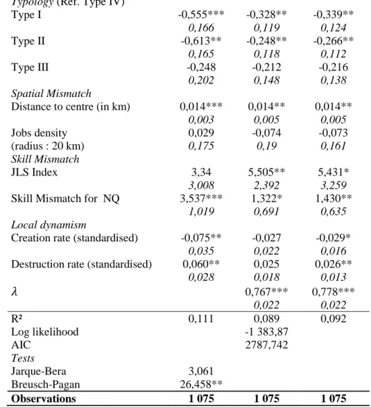
Firstly, we present the results of the estimations without distinguishing between the different spatial regimes (Table 4). The first column presents the results of an OLS model with the use of the matrix of variance-covariance corrected for heteroscedasticity by the White procedure. The Breusch-Pagan test (White test) effectively reveals the presence of heteroscedasticity in the model and requires us to take it into account8. The Jarque-Bera test shows, for its part, that the residuals of the model follow normal distribution9.

Firstly, we observe that the socio-economic composition determines the chances of exit from unemployment in the towns. Towns that are considered the most disadvantaged by their characteristics are the localities the most disadvantaged for a rapid exit from unemployment. Conversely, the most advantaged towns by composition (types I and II) are those where the observed durations of unemployment are lowest. However, concerning these indicators, two limitations must be kept in mind. Firstly, we cannot say which characteristics of this summary indicator contribute the most to explain unemployment duration. Secondly, it is difficult to say if it is the specific characteristics of each individual that have an effect (for example, the fact of being a manager) or more the external factors due to the composition of the neighbourhood (the fact of having managers as neighbours).

Concerning the Spatial Mismatch indicators, we see that the distance to the centre increases the average duration of unemployment. So the furthest towns from the principal centre of employment are equally those confronted with the longest durations. This fact suggests that poor accessibility to jobs is effectively a brake on the exit from unemployment because it impedes the process of finding a job. This result is in line with those already found by GOBILLON and SELOD (2007), DUGUET et al.(2009). The density of jobs (understood as

8 _{The null hypothesis is that of homoskedasticity. We reject the null 'hypothesis if the test statistic (nR²) is higher}

than the value obtained in the Khi-deux table. See chapter 8 in the book of WOOLDRIDGE (2002).

9 _{The null hypothesis is that the residuals of the model follow normal distribution. To know if we accept this}

hypothesis, we compare the Jarque-Bera statistic with that in the Khi-deux table at two degrees of freedom. If the estimated value of the Jarque-Bera statistic is lower, we accept the null hypothesis.

the ratio between jobs and labour force) in a radius of 20 kilometres shows no significant effect. The relative abundance of jobs locally and/or the potential competition in the workforce does not seem to have an impact on the average duration of unemployment. The indicators used to measure the Skill Mismatch problem show the same thrust. However, we observe an effect both positive and significant uniquely for our indicator of poor matching of skills for the unqualified (NQ). If there is a problem of matching between skills offered and demanded, it essentially concerns the unqualified.

Finally, we find that local dynamism has a significant impact on unemployment duration disparities. Living in a town where the rate of job creation is high tends to decrease the duration, while a high rate of destruction increases it. This can be explained by weak local dynamism that decreases the chances of finding a job. The two others columns in Table 4 present the results of the SEM model. The second and third columns present the results estimated by the Maximum-Likelihood method (ML) and by the generalised method of moments (GMM) respectively. Whatever the method, we see that G is positive and significant at the 1% level. This shows the importance of auto-correlation problem in what concerns error terms and so the necessity of taking it into account in our estimations. Globally, the results are the same as in the model estimated by OLS. We see that the indicator inspired by Jackman, Layard and Savouri to measure Skill Mismatch is now significant. The problem of mismatch does not only concern the unqualified, but all the levels of qualification. It is likely that its effect is partially absorbed by the effect of the unqualified’s own mismatch. Finally, let us note that the effect of local dynamism is sensitive to the method of estimation used because, if the signs and the sized observed do not change, their significativity varies from one estimation to another.

Table 4. Explaining the durations of unemployment

Variables OLS-White SEM-ML SEM-GMM

Constant 10,124*** 10,281*** 10,278***

Typology (Ref. Type IV) Type I -0,555*** -0,328** -0,339** 0,166 0,119 0,124 Type II -0,613** -0,248** -0,266** 0,165 0,118 0,112 Type III -0,248 -0,212 -0,216 0,202 0,148 0,138 Spatial Mismatch

Distance to centre (in km) 0,014*** 0,014** 0,014**

0,003 0,005 0,005 Jobs density 0,029 -0,074 -0,073 (radius : 20 km) 0,175 0,19 0,161 Skill Mismatch JLS Index 3,34 5,505** 5,431* 3,008 2,392 3,259

Skill Mismatch for NQ 3,537*** 1,322* 1,430**

1,019 0,691 0,635 Local dynamism

Creation rate (standardised) -0,075** -0,027 -0,029*

0,035 0,022 0,016

Destruction rate (standardised) 0,060** 0,025 0,026**

0,028 0,018 0,013 G 0,767*** 0,778*** 0,022 0,022 R² 0,111 0,089 0,092 Log likelihood -1 383,87 AIC 2787,742 Tests Jarque-Bera 3,061 Breusch-Pagan 26,458** Observations 1 075 1 075 1 075

Sources :Pôle emploi FHS, DADS 2002-2005, population census 1999 (INSEE).

Notes : ***, ** and * denote significance at the 1%, 5% and 10% levels respectively. Standard

deviations presented in italics.

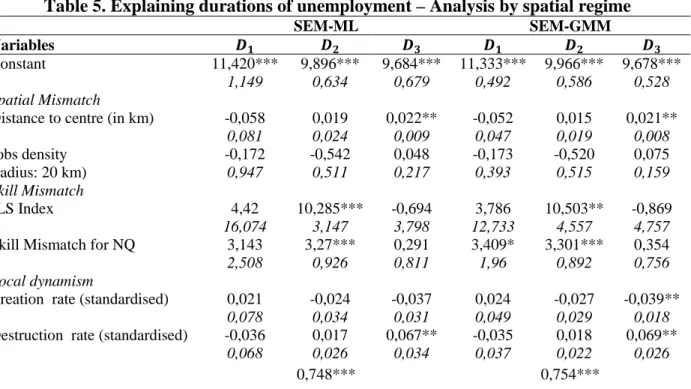
Table 5 presents the result of our estimations with a spatial regimes model. We recall that each regime is determined by its distance from the centre (see previous section for more details)10. The estimations are done by the Maximum-Likelihood Method and the Generalised Moments Method. The typology of the towns is not introduced here because the distribution within the different types of towns conflicts with the arrangement of spatial regimes. We show in Annex D that the results are not really affected by the introduction of our socio-economic composition indicator.

10 _{We have tested different spatial regimes to verify the robustness of our results. With only two regimes, we}

have on one side the towns whose distance is less than 39 kilometres from the centre (50% of our sample) and on the other the towns whose distance is more (also 50%). The results are globally close to those we find in distinguishing the three regimes.

Overall, although few of the variables show significant effects, we observe a certain number of differences between the regimes and so the localities of the towns. It would appear that the problems of Skill Mismatch (for the whole population or only the unqualified) exclusively concern the towns near the centre of Paris. These problems no longer arise when we look at the third regime, which includes the 50% of the towns furthest from the centre. Conversely, if the proximity to the principal employment centre does not seem to be an advantage for jobseekers living there, it does however represent a net disadvantage for the residents of the most distant towns. For the towns beyond a radius of 39 kilometres, we can note that going a little further increases the duration of unemployment. Finally, local employment dynamism also influences the average duration of unemployment, but exclusively for the furthest towns. We could suppose that the rates of creation and destruction have only minor importance for the residents of towns close to a considerable source of jobs. On the other hand, this is an important factor for those concerned by poor physical access to jobs and/or who have more limited job opportunities than others.

Table 5. Explaining durations of unemployment – Analysis by spatial regime

SEM-ML SEM-GMM

Variables ^_{_} ^_{`</sub> ^<sub>a</sub> ^<sub>_</sub> ^<sub>`} ^_a

Constant 11,420*** 9,896*** 9,684*** 11,333*** 9,966*** 9,678***

1,149 0,634 0,679 0,492 0,586 0,528

Spatial Mismatch

Distance to centre (in km) -0,058 0,019 0,022** -0,052 0,015 0,021**

0,081 0,024 0,009 0,047 0,019 0,008 Jobs density -0,172 -0,542 0,048 -0,173 -0,520 0,075 (radius: 20 km) 0,947 0,511 0,217 0,393 0,515 0,159 Skill Mismatch JLS Index 4,42 10,285*** -0,694 3,786 10,503** -0,869 16,074 3,147 3,798 12,733 4,557 4,757

Skill Mismatch for NQ 3,143 3,27*** 0,291 3,409* 3,301*** 0,354

2,508 0,926 0,811 1,96 0,892 0,756

Local dynamism

Creation rate (standardised) 0,021 -0,024 -0,037 0,024 -0,027 -0,039**

0,078 0,034 0,031 0,049 0,029 0,018

Destruction rate (standardised) -0,036 0,017 0,067** -0,035 0,018 0,069**

0,068 0,026 0,034 0,037 0,022 0,026

0,023 0,024 KL _{0,384 0,741 0,647} R² 0,169 0,172 Log likelihood -1 373,35 AIC 2 788,70 Tests Chow 29,930** 51,179*** Observations 110 429 536 110 429 536

Sources :Pôle Emploi FHS, DADS 2002-2005, population census 1999 (INSEE).

Notes: ***, ** and * denote significance at the 1%, 5% and 10% levels respectively. Standard

deviations in italics.

Using these estimations with spatial regimes permits to highlight the differentiated effects of the explanations of unemployment duration disparities. The problems of Skill Mismatch seem to affect more the towns close to the centre of Paris, whereas the problems of Spatial Mismatch are more evident for the towns the furthest from this centre. We must bear this distinction in mind when we suggest public policy solutions.

C

The residents of central Paris are confronted with an abnormally long duration of unemployment. In the middle of the 2000s, the duration of unemployment was 14 months in Paris compared to 11.5 months in the Paris region and 10.5 months for France. Paris was the French department where the proportion of jobseekers of more than a year among the total jobseekers was the highest before the crisis. Paris is not an optimal location from the point of view of return-to-employment, all things being equal. A fringe location, in the inner ring or on the edge of the metropolitan area, but without going too far, is preferrable for reducing the duration of unemployment of a jobseeker.

The objective of this work is to explain this overexposure of Parisians to long-term unemployment. It is to find a factor that affects all the categories of jobseeker, whatever their age, sex, nationality, level of educational qualifications, marital situation, number of children,

type of contract sought, trade sought, reason for entering unemployment, all the control variables we use to measure the durations of unemployment. We also seek a sufficiently important factor to have a significant effect on the individual durations of unemployment of 110,000 Parisian jobseekers, and sufficiently durable to exercise an effect over the last 30 years.

The explanation that we offer combines two theoretical mechanisms, Spatial Mismatch and Skill Mismatch. Parisian jobseekers live close to a high-volume source of jobs but the characteristics of the jobs offered do not correspond to those of jobs sought. However, the job offers that do effectively correspond to the characteristics of jobseekers are generally physically far from the centre of Paris, in the intermediate ring of the Paris metropolitan area. Then, Parisian jobseekers experience a longer jobsearch time than jobseekers of other towns and departments.

This explanation does not exclude other factors playing a role, without us being able to furnish empirical evidence. For example, the Paris stock of public housing could contribute to limiting the geographic mobility of jobseekers. According to the City of Paris, this stock includes 183,500 dwellings subsidised by the central government, the City and the region, to which we add 56,000 intermediate dwellings managed by providers of social housing, but the annual offer is limited to 13,000. Therefore it is very difficult to accede to public housing in Paris, which gives it a higher importance and promotes geographical immobility, which then reduces the perimetre of a jobsearch and increases its duration. The welfare policies of the City of Paris, informal work in the hotels-cafés-restaurants sector and in culture, or even the problems of employment policy in Paris, constitute other factors that could also contribute to lengthening the Parisian duration of unemployment.

References

ARNOTT R. (1998), «Economic theory and the Spatial Mismatch hypothesis», Urban Studies,

BAUDER H. et PERLE E. (1999), «Spatial and skills mismatch for labor market segments»,

Environment and Planning A, 31(6), pp. 959-979.

BOUABDALLAH K., CAVACO S. et LESUEUR J-Y. (2002), « Recherche d’emploi, contraintes

spatiales et durée du chômage : une analyse microéconométrique », Revue d’économie politique, n° 1, pp. 137-157.

BRUECKNER J. et ZENOU Y. (2003), «Space and Unemployment: The labour-Market effects of Spatial Mismatch», Journal of Labour Economics, 21(1), pp. 242-262.

CARLSON V. et THEODORE N. (1995), «Are There Enough Jobs? Welfare Reform and Labor Market Reality», Chicago: Illinois Job Gap Project.

CAVACO S. et LESUEUR J-Y. (2004), « Contraintes spatiales et durée de chômage », Revue Française d'Economie, 18(3), pp. 229-257.

COULSON E., LAING D. et WANG P. (2001), «Spatial mismatch in Search Equilibrium»,

Journal of Labour Economics, 19, pp. 949-972.

DANZIGER S. et HOLZER H., «Are Jobs Available for Disadvantages Groups in Urban

Areas?», Working paper, Michigan State University and University of Michigan, 97-406. DAVIS S. et HALTIWANGER J. (1990), «Gross Job Creation and Destruction: Microeconomic

Evidence and Macroeconomic Implications», NBER Macroeconomics Annual.

DAVIS S. et HUFF D. (1972), «Impact of Ghettoization on Black Employment», Economic

Geography, 48, pp. 421-447.

DÉTANG-DESSENDRE C. et GAIGNÉ C. (2009), «Unemployment Duration, City Size, and the

Tightness of the Labor Market», Regional Science and Urban Economics, 39(3), pp. 266-276. DUGUET E., GOUJARD A. ET L'HORTY Y. (2009), « Les inégalités territoriales d'accès à

l'emploi : une exploration à partir de sources administratives exhaustives », Economie et Statistique, 415-416, pp. 17-44.

DUGUET E.,L'HORTY Y. ET SARI F. (2009), « Sortir du chômage en Ile-de-France, Disparités territoriales, spatial mismatch et ségrégation résidentielle», Revue Economique, 60(4), pp. 979-1010.

GASCHET F. et GAUSSIER N. (2004), «Urban segregation and labour markets within the

Bordeaux metropolitan area: an investigation of the spatial friction», Working Papers of gres, Cahiers du gres, vol. 19.

GOBILLON L., MAGNAC T. et SELOD H. (2011), «The Effect of Location on Finding a Job in the Paris Region», Journal of Applied Econometrics, 26(7), pp. 1079-1112.

GOBILLON L. et SELOD H. (2007), « Ségrégation résidentielle, accès à l’emploi et chômage : le cas de l’Ile-de-France », Economie et Prévision, 180-181, pp. 19-38.

GOBILLON L., SELOD H. et ZENOU Y. (2007), «The Mechanisms of Spatial Mismatch», Urban Studies, 44(12), pp. 2401-2427.

GORDON I. (2002), «Unemployment and Spatial Labour Markets: Strong Adjustment and

Persistent Concentration», in Ron M. et Morrison P., (eds.), Geographies of Labour Market Inequality. Regional development and public policy, London: Taylor and Francis.

HOUSTON D. (2005), «Employability, Skills Mismatch and Spatial Mismatch in Metropolitan Labour Markets», Urban Studies, 42(2), pp. 221-243.

IHLANDFELT K. et SJOQUIST D. (1990), «Job Accessibility and Racial Differences in Youth Employment Rates», The American Economic Review, 80(1), pp. 267-276.

IHLANDFELT K. et SJOQUIST D. (1991), «The Effect of Job Access on Black and White Youth Employment: A Cross-Sectional Analysis», urban Studies, 28 (2), pp. 255-265.

JACKMAN R.,LAYARD R. ET SAVOURI S. (1990), «Labour Market Mismatch: a Framework of

Though», in Paoda-Schioppa F. (eds), Mismatch and Labor Mobility, Cambridge University Press.

JAYET H. (1993), Analyse Spatiale Quatitative, Une Introduction, Paris, Economica.

KAIN J. (1968), «Housing Segregation, Negro Employment, and Metropolitan

Decentralization», Quarterly Journal of Economics, 82, pp.175-197.

KORSU E. et WENGLENSKI S. (2010), «Job Accessibility, Residential Segregation and Risk of

Long-Term Unemployment in Paris Region», Urban Studies, 47(10), pp.2279-2324.

LE GALLO J. (2002), « Économétrie spatiale : l’auto-corrélation spatiale dans les modèles de régression linéaire », Économie et Prévision, 155, p. 139-157.

LE GALLO J. (2004), « Hétérogénéité spatiale, principes et méthodes », Economie et Prévision, 162, pp. 151–172.

LESAGE J.P. (1998), «Spatial Econometrics», Université de Tolède, Mimeo.

MANACORDA M. et PETRONGOLO B., «Skill Mismatch and Unemployment in OECD Countries», Economica, 66, pp. 181-207.

PASTOR J. et MARCELLI E. (2000), «Men in the hood: Skill, Spatial, and Social Mismatches among Male Workers in Los Angeles County», Urban Geography, 21(6), pp. 474-496.

ROGERS C. (1997), «Job Search and Unemployment Duration: Implications for the Spatial Mismatch Hypothesis», Journal of urban Economics, 42(1), pp. 109-132.

RUPERT P., STANCANELLI E. et WASMER E. (2009) «Commuting, Wages and Bargaining Power», Annales d'Économie et de Statistiques, 95-96, pp. 201-221.

STOLL M. (2005), «Geographical Skills Mismatch, Job Search and Race», Urban Studies,

42(4), pp. 695-717.

THISSE J-F. et ZENOU Y. (2000), « Skill Mismatch and Unemployment », Economics Letters,

69, pp. 415-420.

WOOLDRIDGE J. (2002), Introductory Economics: A Modern Approach, South-Western

Annexes

Annex A. Individual determinants of exits from unemployment

Removal from list Return to work Coefficient Student Coefficient Student

α 0,917 2252,53 0,843 1148,88 Age (years) -0,018 236,17 -0,036 234,27 Permanent contract réf réf Limited-term contract -0,382 125,96 -0,491 87,52 Seasonal -0,104 37,21 -0,168 31,29 Degree level VI réf réf Level I et II -0,001 0,40 0,364 59,17 Level III 0,032 11,30 0,361 66,17 Level IV -0,030 13,02 0,186 40,06 Level V -0,051 30,29 0,074 19,93 Without children réf réf One child -0,077 41,31 0,017 4,50 Two children -0,079 37,41 0,224 56,22 Three or more children -0,055 22,75 0,235 47,71

Man réf réf Woman -0,062 40,20 -0,223 77,02 Non disabled réf réf Disabled -0,274 98,01 -0,621 94,96 Single, widowed réf réf Divorced, separated 0,031 12,44 -0,009 1,83 Married, de facto married -0,003 1,51 -0,011 3,21

ROME : Serv persons and community réf réf

Administrative and sales 0,024 10,00 0,039 8,01 Hotels restaurants 0,313 105,82 0,499 84,00 Sales and distribution 0,124 52,34 0,151 30,27 Arts and entertainment -0,523 102,18 -1,013 86,48 Initial and continuing education -0,073 13,71 -0,072 7,56 Social work devt local employment 0,042 11,06 0,022 2,93 Paramedical 0,205 37,32 0,315 31,95 Medical 0,025 2,16 0,144 7,26 Managers admin/ communic. information -0,060 15,70 -0,090 12,47 Managers sales -0,028 6,21 -0,004 0,50 Agriculture and fisheries 0,102 24,17 0,229 27,35 Public works and extraction 0,190 55,82 0,323 45,34 Transport and logistics 0,010 3,66 0,096 16,82 Mechanical electrical electronic 0,049 14,74 0,094 14,20 Processing -0,088 20,16 -0,010 1,20 Other manufacturing 0,005 0,97 0,113 9,89 Personal artisanal 0,206 45,12 0,309 34,14 Industrial management 0,117 8,61 -1,873 153,72 Industrial technician 0,037 8,31 0,002 0,20 Management technical industries 0,069 12,28 0,080 8,25 Technical managers outside

manufacturing 0,146 27,45 0,195 20,66

Lay-offs for financial reasons réf réf

Other lay-offs 0,053 18,65 -0,042 8,27 Resignations 0,507 153,49 0,389 63,94 End of contracts 0,292 110,40 0,421 89,42 End of temp work 0,275 86,04 0,236 39,60 First entry 0,568 166,56 0,363 53,66 Return to work of more than 6 months 0,489 115,46 0,309 35,25 Other cases 0,367 137,21 0,153 30,34

Manual workers réf réf

Unskilled employees -0,008 3,34 -0,051 9,25 Skilled employees -0,025 10,17 0,144 27,55 Technician, supervisor -0,003 0,96 0,204 30,85 Manager -0,030 6,99 0,155 18,80 Non RMI réf réf RMI -0,212 105,27 -0,587 114,12 Full-time réf réf Part-time -0,226 120,70 -0,555 132,22 Nationality French réf réf EU 15 0,066 14,39 0,094 10,35 Rest of world -0,002 0,79 -0,197 35,26

Reading :Results of estimations of Weibull model by Maximum-Likelihood. The coefficients apply to rates of exit

from unemployment (i.e. hazard function) in relation to the modality of reference indicated in the table.

Annex B. Results of ACP and CAH

Table B-1. Coordinates, contributions et cosines squared of variables

Coordonates Contributions Cosines squared Variables Axis 1 Axis 2 Axis 1 Axis 2 Axis 1 Axis 2

Proportion of families with

foreigner head -0,12 -0,84 0,45 34,03 0,02 0,70 Proportion of single-parent families -0,08 -0,75 0,19 27,23 0,01 0,56 Proportion of pers. Low qualified -0,68 0,53 13,40 13,36 0,47 0,28 Proportion of pers.. >High school

diploma +2 years 0,81 0,05 19,01 0,11 0,66 0,00 Proportion of managers 0,90 -0,16 23,18 1,32 0,81 0,03 Proportion of manual workers -0,82 0,11 19,43 0,59 0,68 0,01 Average income 0,78 0,07 17,51 0,25 0,61 0,01 Unemployment rate -0,49 -0,69 6,83 23,12 0,24 0,48

Source : population census INSEE (1999).

Fields : Analysis in principal components effected on 1300 towns of Ile-de-France region.

Table B-2. Descriptive statistics of types of towns used for CAH.

Type I Type II Type III Type IV Total

Variables Av. Standard-deviation Av. Standard-deviation Av. Standard-deviation Av. Standard-deviation Av. Standard-deviation

Proportion of families with

foreigner head 7,14 0,04 5,37 0,03 4,69 0,03 16,49 0,06 6,38 0,05

Proportion of single-parent

families 9,85 0,05 8,42 0,04 7,45 0,05 16,39 0,03 9 0,05

Proportion of pers. Low

qualified 14,34 0,04 23,22 0,03 26,54 0,04 21,16 0,03 22,99 0,05

Proportion of pers.. >High

school diplom+2 12,31 0,02 10,56 0,02 6,73 0,02 7,14 0,02 9,18 0,03

Proportion of managers 42,12 0,09 20,63 0,07 10,5 0,05 12,28 0,07 19,25 0,12

Proportion of manual workers _{9,75 0,05 18,51 0,05 32,21 0,09 27,59 0,07 22,84 0,11} Average income 37 417 13 778 23 487 3 787 19 944 3 275 15 545 2 538 23 394 8 418

Unemployment rate _{7,39 0,02 7,38 0,02 9,26 0,03 15,61 0,03 8,77 0,03}

Number of towns 171 569 442 118 1300

Source : population census INSEE (1999).

TEPP Working Papers 2014

14_17. he impact of a disability on labour market status: A comparison of the public and private sectors

Thomas Barnay, Emmanuel Duguet, Christine Le Clainche, Mathieu Narcy, Yann Videau

14_16. Employer-provided health insurance and equilibrium wages with two-sided heterogeneity

Arnaud Chéron, Pierre-Jean Messe, Jérôme Ronchetti

14_15. Does subsidising young people to learn to drive promote social inclusion? Evidence from a large controlled experiment in France

Julie Le Gallo, Yannick L'Horty, Pascale Petit

14_14. Hiring discrimination based on national origin and the competition between employed and unemployed job seekers

Guillaume Pierné

14_13. Discrimination in Hiring: The curse of motorcycle women

Loïc Du Parquet, Emmanuel Duguet, Yannick L'Horty, Pascale Petit

14_12. Residential discrimination and the ethnic origin: An experimental assessment in the Paris suburbs

Emmanuel Duguet, Yannick L'Horty, Pascale Petit

14_11. Discrimination based on place of residence and access to employment

Mathieu Bunel, Yannick L'Horty, Pascale Petit

14_10. Rural Electrification and Household Labor Supply: Evidence from Nigeria

Claire Salmon, Jeremy Tanguy

14_9. Effects of immigration in frictional labor markets: theory and empirical evidence from EU countries

Eva Moreno-Galbis, Ahmed Tritah

14_8. Health, Work and Working Conditions: A Review of the European Economic Literature

Thomas Barnay

14_7. Labour mobility and the informal sector in Algeria: a cross-sectional comparison (2007-2012)

Philippe Adair, Youghourta Bellache

14_6. Does care to dependent elderly people living at home increase their mental health?

Thomas Barnay, Sandrine Juin

14_5. The Effect of Non-Work Related Health Events on Career Outcomes: An Evaluation in the French Labor Market

Emmanuel Duguet, Christine le Clainche

14_4. Retirement intentions in the presence of technological change: Theory and evidence from France

Pierre-Jean Messe, Eva Moreno – Galbis, Francois-Charles Wolff

14_3. Why is Old Workers’ Labor Market more Volatile? Unemployment Fluctuations over the Life-Cycle

Jean-Olivier Hairault, François Langot, Thepthida Sopraseuth

14_2. Participation, Recruitment Selection, and the Minimum Wage

Frédéric Gavrel

14_1. Disparities in taking sick leave between sectors of activity in France: a longitudinal analysis of administrative data