Imaging spectroscopy for soil mapping and monitoring

HAL Id: hal-02735880

https://hal.inrae.fr/hal-02735880

Submitted on 2 Jun 2020

HAL is a multi-disciplinary open access

archive for the deposit and dissemination of

sci-entific research documents, whether they are

pub-lished or not. The documents may come from

teaching and research institutions in France or

abroad, or from public or private research centers.

L’archive ouverte pluridisciplinaire HAL, est

destinée au dépôt et à la diffusion de documents

scientifiques de niveau recherche, publiés ou non,

émanant des établissements d’enseignement et de

recherche français ou étrangers, des laboratoires

publics ou privés.

S. Chabrillat, E. Ben-Dor, J. Cierniewski, Cécile Gomez, T. Schmid, B. van

Wesemael

To cite this version:

S. Chabrillat, E. Ben-Dor, J. Cierniewski, Cécile Gomez, T. Schmid, et al.. Imaging spectroscopy for

soil mapping and monitoring. Surveys in Geophysics, Springer Verlag (Germany), 2019, Proceedings

of the Workshop on Exploring the Earth’s Ecosystems on a Global Scale - Requirements, Capabilities

and Directions in Space borne Imaging Spectroscopy, 40, pp.361-399. �10.1007/s10712-019-09524-0�.

�hal-02735880�

Imaging Spectroscopy for Soil Mapping and Monitoring

B. van Wesemael6

Received: 16 February 2018 / Accepted: 28 February 2019 / Published online: 20 March 2019 © Springer Nature B.V. 2019

Abstract

There is a renewed awareness of the finite nature of the world’s soil resources, growing concern about soil security and significant uncertainties about the carrying capacity of the planet. Regular assessments of soil conditions from local through to global scales are requested, and there is a clear demand for accurate, up-to-date and spatially referenced soil information by the modelling scientific community, farmers and land users, and policy- and decision-makers. Soil and imaging spectroscopy, based on visible–near-infrared and short-wave infrared (400–2500 nm) spectral reflectance, has been shown to be a proven method for the quantitative prediction of key soil surface properties. With the upcoming launch of the next generation of hyperspectral satellite sensors in the next years, a high potential to meet the demand for global soil mapping and monitoring is appearing. In this paper, we briefly review the basic concepts of soil spectroscopy with a special attention to the effects of soil roughness on reflectance and then provide a review of state of the art, achievements and perspectives in soil mapping and monitoring based on imaging spectroscopy from air- and spaceborne sensors. Selected application cases are presented for the modelling of soil organic carbon, mineralogical composition, topsoil water content and characterization of soil crust, soil erosion and soil degradation stages based on airborne and simulated spa-ceborne imaging spectroscopy data. Further, current challenges, gaps and new directions toward enhanced soil properties modelling are presented. Overall, this paper highlights the potential and limitations of multiscale imaging spectroscopy nowadays for soil mapping and monitoring, and capabilities and requirements of upcoming spaceborne sensors as sup-port for a more informed and sustainable use of our world’s soil resources.

Keywords Soil mapping and monitoring · Imaging spectroscopy · Hyperspectral · Soil organic carbon · Soil mineralogical composition · Surface roughness · Soil moisture · Vegetation cover · Spaceborne instruments

* S. Chabrillat

sabine.chabrillat@gfz-potsdam.de

1 Introduction

“All natural resources… are soil or derivatives of soil. Farms, ranges, crops, and livestock, forests, irrigation water and even water power resolve themselves into questions of soil. Soil is therefore the basic natural resource” said Aldo Leopold in 1921 “Erosion and Pros-perity” (Meine and Knight 1999). Nearly all of the food, fuel and fibres used by humans are produced on soil. Soil is also essential for water and ecosystem health. It is second only to the oceans as a global carbon sink, with an important role in the potential slowing of cli-mate change. Several soil functions depend on a multitude of soil organisms, which makes soil an important part of our biodiversity. Nowadays, in the face of rapidly growing popula-tion, there is a renewed awareness of the finite nature of the world’s soil resources (Harte-mink and McBratney 2008), growing concern about soil security (FAO and ITPS 2015) and significant uncertainties about the carrying capacity of the planet (i.e. the number of people that the Earth can support (UNEP 2012)). Hartemink (2008) further acknowledged “Soils are back on the global agenda”. This growing concern has been answered with a growing number of soil policies and regulations around the world concerned with, e.g., increasing soil degradation and loss of organic carbon in topsoils and aiming at more soil management and soil protection such as the EU Soil Thematic Strategy and Soil Frame-work Directive. The European Commission recognized that soil resources in many parts of Europe are being over‐exploited, degraded and irreversibly lost due to inappropriate land management practices, industrial activities and land‐use changes that lead to soil sealing, contamination, erosion and loss of organic carbon (JRC 2012). Soil scientists are being challenged to provide assessments of soil conditions from local to global scales (Grunwald et al. 2011; Arrouays et al. 2017). However, only a few countries have the necessary survey and monitoring programs to meet these new needs and existing global data sets are out of date. For example, the state-of-the-art Harmonized World Soil Database (FAO 2012) providing up-to-date information on world soil resources at approximately 1 km scale (30 arc-second database) was last updated in 2013 and recognizes that the reliability of the information contained in the database is variable. A particular issue is the clear demand for a new regional to global coverage with accurate, up-to-date and spatially referenced soil information as expressed by the scientific community, farmers and land users, and policy- and decision-makers (EC 2006).

In this regard, optical remote sensing observations and in particular reflectance spectroscopy at the remote sensing scale, referred to as imaging spectroscopy (IS), or hyperspectral imaging, have been shown to be powerful techniques for the quantitative determination and modelling of a range of soil properties. These soil properties include topsoil mineralogical composition such as soil organic carbon (SOC) content, textural composition, iron or carbonate content, etc., and physical attributes (e.g., Ben-Dor et al. 2009). The attractiveness of imaging spectroscopy is that measurements are rapid and estimates of soil properties are inexpensive compared to conventional soil analyses, as it exploits the information carried out by the visible and near-infrared (Vis–NIR: 400–1100 nm) and shortwave infrared (SWIR: 1100–2500 nm) part of the electromag-netic spectrum (Goetz et al. 1985). IS has been used since more than 20 years in vari-ous soil applications such as evaluation and monitoring of soil quality and soil function (e.g., soil moisture and carbon storage), soil fertility and soil threats (e.g., acidification and erosion) and soil pedogenesis (i.e. soil formation and evolution). Further, soil deg-radation (salinity, erosion and deposition), soil mapping and classification, soil genesis and formation, soil contamination and soil hazards (swelling soils) are also important

soil science issues nowadays examined with IS, enlarging the soil spectroscopy into the spatial domain from mainly airborne platforms (e.g., see review of Ben-Dor et al. 2018). Research on quantitative soil spectroscopy for the prediction of soil properties has largely benefited from technological and methodological developments over the past decades. The availability of new high signal-to-noise ratio airborne hyperspectral sen-sors allowed the delivery, at remote sensing scale, of laboratory-like reflectance data. Simultaneously, developments in multivariate statistics and chemometrics opened sig-nificant new possibilities toward soil spectral modelling and quantitative analyses of the physical and biochemical composition of the Earth’s soil based on spectral reflectance.

In the upcoming future, a large availability of high signal-to-noise ratio satellite imaging spectrometers is expected. Several target missions having high spatial resolution and limited coverage per day are soon to be launched such as the Italian PRISMA (PRecursore IperS-pettrale della Missione Applicativa) (Loizzo et  al. 2018), launch 2019, 30  m; the German EnMAP (Environmental Mapping and Analysis Program) (Guanter et al. 2015), launch 2020, 30 m; the Japanese HISUI (Hyperspectral Imager Suite) (Matsunaga et al. 2018), to be put on the International Space Station in 2019, 30 m; and the Italy–Israeli SHALOM (Spaceborne Hyperspectral Applicative Land and Ocean Mission) (Ben-Dor et al. 2014), launch 2024, pos-sibly 10 m. Among these missions, the open data policy of the German EnMAP mission is worth noting. Furthermore, several global mapping missions are planned or under study for the upcoming future such as the NASA-SBG (Surface Biology and Geology), former HyspIRI mission (Lee et al. 2015; Green 2018), HySpex2 proposed as Earth Explorer Mission ESA (Briottet et al. 2017) and the Sentinel-10/CHIME satellite proposed as ESA candidate mission (Copernicus Hyperspectral Imaging Mission for the Environment) (Rast et al. 2019). These satellites with their variable spatial coverage and different ground sampling distances will rep-resent for soil scientists a major step toward global soil mapping and monitoring as a response to the need for accurate, up-to-date information on the world’s state of soils.

Nevertheless, to be able to answer that demand and to reach the full potential of imag-ing spectroscopy from orbital utilization for soil mappimag-ing, challenges have been identified and, for example, linked to limitations in reference data availability (e.g., global standard-ized soil spectral libraries databases) and in methodological approaches and tools adequate to process the spectral data into practical soil model solutions that are globally applicable (e.g., Ben-Dor et al. 2018). An area of active research nowadays is thus on the demonstra-tion of the potential and limitademonstra-tions of hyperspectral imagery for soil mapping and moni-toring from airborne to spaceborne scale and on the development of enhanced databases and methods to be ready for upcoming hyperspectral satellite launches with adapted strate-gies and tools for the computation and delivery of global soil maps.

In this frame, we present in this paper a timely review of state of the art, challenges and limitations of imaging spectroscopy for soil applications, for young and senior research schol-ars, undergraduate and graduate students in Earth sciences and remote sensing, soil scientists, institutional and industrial soil entities that are concerned with the future use of remote sens-ing data for soil mappsens-ing and monitorsens-ing. This paper is divided into three sections. First, a review of basic concepts of soil spectroscopy for soil properties’ determination is presented, including a thorough review of the effect of soil roughness on reflectance. Then, a review of the applications of imaging spectroscopy for the mapping of soil properties is presented, including selected application cases demonstrating the potential and limitations of imaging spectroscopy for the mapping of SOC, common soil properties, soil moisture, soil crust, soil erosion and degradation. Finally, a review of current challenges and gaps related to the use of air- to spaceborne imaging spectroscopy data is presented and discussed in view of future avenues of research, perspectives and user requirements for upcoming satellites.

2 Theory and Concepts

2.1 Principles of Soil Spectroscopy for Soil Properties Identification and Modelling

The soil reflectance spectrum (ρ) is a collection of values obtained at every spectral band (λ) from the ratio of radiance (E) and irradiance (L) fluxes across most of the spectral region of the solar emittance function. The reflectance values are traditionally described, from a practical standpoint, by a relative ratio against a perfect reflector spectrum meas-ured at the same geometry and position of the soils (Palmer 1982; Baumgardner et  al. 1985; Jackson et al. 1987). The reflectance information is used to identify material by the nature of the reflectance spectrum it provides. The more wavelengths involved in the meas-urement scheme, the more information can be obtained. The nature of the spectrum is com-posed of absorption features of chemical constituents (“peaks”) (e.g., absorption of OH of water molecules) and overall spectral shape of the physical properties (“albedo”) (e.g., particle size) (Ben-Dor and Banin 1995a, b).

In soils, the optical activity of chemical chromophores (i.e. those parts of a molecule responsible for its colour) is due to vibration overtones and combination modes of func-tional groups at the molecular level across the SWIR spectral region and to electronic transitions in atoms across the Vis–NIR spectral regions at specific wavelengths. A com-pressive description on the exact soil chromophore and its electromagnetic activity can be found in, e.g., Ben-Dor et al. (1999), Stenberg et al. (2015), Demattê et al. (2015). The physical chromophores are due to scattering effects based on particle size and shape dis-tribution in the material. The water molecule influences the absorption features at specific wavelengths that are the results of overtone and combination modes from the IR region as well as the results of the physical effects that scatter the light in a way that the spectrum shape and base line are changing. Figure 1 provides a typical soil spectrum with the direct known chromophores. It can be seen that there are physical (baseline height and spectral shape) and chemical (absorption) features. In the Vis–NIR region, electronic transitions are dominated mainly in iron oxides with also organic matter (OM) that refer to the slope of the spectrum part (probably related to soil OM structure). In the SWIR region, the water

Fig. 1 A soil spectrum (Haploxeralf) that represents the major chromophores in soils (after Ben-Dor et al. 2008)

molecules in hygroscopic water play a major role in 1.4 and 1.9 µm where clay minerals and calcite are at around 2.2 and 2.3 µm, respectively. The wavelengths may vary based on the structure of the minerals and their crystal shape and purity. All possible absorption fea-tures and their quantum mechanisms in the Earth’s crust minerals were summarized, e.g., in Ben-Dor et al. (1999).

Soil is a complex system that is extremely variable in physical structure and chemical composition both temporally and spatially. Soil spectroscopy, although being complex, can cluster several soil properties with a single measurement that can be extracted based on radi-ative transfer models (e.g., Hapke 1981) or empirical data-mining (chemometric) approach (Ben-Dor and Banin 1995b). The prediction of a soil spectrum from physical bases is quite difficult (Liang and Townshend 1996). Each soil property Si has to respect the following

rules to be successfully predicted by soil spectroscopy: Rule (1.1) the soil property Si has

a specific spectral signature due to a chemical or physical structure (Ben-Dor et al. 2002) or Rule (1.2) the soil property Si is correlated with a soil property Sj having a specific

spec-tral signature due to an associated chemical or physical structure (Ben-Dor et  al. 2002); and additionally Rule (2) the soil property Si has to have a quite high amount of variability

(Gomez et al. 2012a, b). Until now, and from our knowledge, the limits of the quantification of a soil property that has got a low variability within the scene have not been explored in detail as this minimum of variability may depend on (1) the studied soil property and (2) the link with other soil properties on the soil samples. This last rule implies that the predictabil-ity of a primary soil property depends on the soil diverspredictabil-ity of the study site. For example, Ben-Dor et al. (2002) had already stressed that the soil is a complex matrix and that the spectral features of one component (e.g., OM) can be hidden or slightly shifted by another component [e.g., iron (hydr)oxides]. Nevertheless, separating the spectral information from the different soil attributes is possible as already shown in previous studies. Laboratory soil spectroscopy, linked with statistical analyses, has, for example, been used since, e.g., the earlier works of Demattê et al. (2004) over soils from São Paulo State, Brazil, for the deriva-tion of soil survey maps and soil classes. It was the first paper applying soil spectroscopy for pedological mapping. The authors developed a spectral reflectance-based methodology that was able to evaluate soil types and soil tillage systems.

Although there is a strong relationship between the soil chromophores as observed in the spectral domain and the chemical/physical characteristics of the material, the correlation is not straightforward. This is because the spectral data are multivariate, with many reciprocal effects (Schwartz et al. 2011). Accordingly, the extraction of quantitative information on a given soil attribute using spectral information is not a simple task, especially if it is not a chromophore attribute. Malley et al. (2004) provided a summary to what soil attributes can be spectrally modelled in soils. In 2006, Rossel et al. extended the application and provided a long list of authors and soil attributes, most of which use chemometric approaches. The chemometric approach is an empirical (statically driven) method, and although no physi-cal, chemical or other assumptions are made, the method has a strong spectroscopic basis, in which the selected bands in the model must have specific assignments. This method provides quantitative information about its chromophore that can be further used. It can be either an index, equation or a model that is extracted from the spectral information, usu-ally combined with the reference information from traditional chemical analyses to “train” the system. Chemometrics also refers to proximate analysis of soil attributes related to the spectral analysis of soil. A sophisticated method of finding this relationship, also known as “data mining”, has to be applied. As the final goal is to use the spectral model for practical remote sensing practices, it is crucial to extract the best model in a given population, rather than just finding a correlation.

Many methods for applying data-mining approach to soil spectral information have been used and developed, from multiple linear regression (MLR) analysis (of the spectra against the chemical/physical data) through principal component analysis regression (Chang et al. 2001), partial least squares regression (PLSR) (Zhao et al. 2015), artificial neural networks (ANN) (Carmon and Ben-Dor 2017) and random forest among others. The standard proce-dure for developing such models will be to divide the samples into calibration and valida-tion sets. The model is then developed on the spectral and chemical data of the calibravalida-tion group and is applied on the spectral data of the validation group to predict its chemical values. The quality of the model is determined by its prediction accuracy using various sta-tistical parameters. When a prediction model with good quality is found, it can be used to predict the chemical values of new samples with just a spectral measurement, either from point or from imaging spectrometers.

As already mentioned, spectral data are affected by various components in the soil, some of which are connected to the chemical property in question, and some not. Thus, applying preprocessing algorithms on the spectra prior to developing the model can amplify relevant spectral features and is traditionally taking place. Manipulation of spectra using derivatives and transformations to log space enables the enhancement of weak spectral features as well as minimizes physical effects (Demetriades-Shah et al. 1990). As a given dataset can be executed using several manipulation stages in a process chain, it is impossible to check many preprocessing combinations manually. Ben-Dor and Banin (1995a) suggested devel-oping a “whole-process” possibility chain in an automated environment to enable optimal data mining, such that the best preprocessing combination could be selected. This concept is termed all possibilities approach (APA), in which all possible combinations are evalu-ated. Moreover, they concluded that aside from good statistical parameters and a selected processing chain, a reliable model must have solid spectral assignments for the spectral region/channels selected by the analysis. This is done by finding the important spectral ranges used by the model and examining whether the selected wavelengths have a mean-ingful explanation based on the physical processes described earlier.

To cope with these challenges, Schwartz et al. (2011) developed a data-mining machine termed “PARACUDA®_{” which runs several preprocessing spectral data manipulations.}

Their concept was based on a smart and single selection of calibration and validation groups from the population in question, using a cubic Latin hypercube sampling algo-rithm for semi-randomized grouping (Minasny and McBratney 2006). Remarkable results were obtained using the PARACUDA machine, mainly due to its automated capability to parallel-check 120 preprocessing combinations. The continued development of the system resulted in the notion that the model quality is sensitive also to the grouping stage and not only to the preprocessing combination. Moreover, the system did not have a viable spectral assignment output, which could significantly amplify the models’ robustness and improve our understanding of the spectral correlations to various soil properties. As the main goal was to develop an accurate (reliable) prediction model, based on finding the best preproc-essing combination and spectral assignments, a new system was recently developed to fully exploit the APA idea of the PARACUDA engine (Carmon and Ben-Dor 2017).

As the quantitative approach of spectral data mining of soils developed, many users are getting into this field and the usage is growing consistently. In this direction, the new machine learning software (such as the PARACUDA-II®_{, Carmon and Ben-Dor 2017) or}

computing approach (such as random forest, Gholizadeh et al. 2015) fosters the use of soil spectroscopy for the quantitative domain. In this case, we examined how many papers have been published during the past 10 years using some keywords of soil spectroscopy (point and image) using Google. An exponential growth in both technologies was found, whereas

the imaging is still lagging behind with respect to point spectroscopy. This is because the soil imaging spectroscopy started later than the point spectroscopy, and only recently has the image technology became more available to more users and the number of papers started to grow. The exponential pattern is not surprising and provides a promising future for the practical use of soil spectroscopy.

It should be pointed out that recently not only the optical domain (Vis–NIR–SWIR) is used for soils but also the thermal infrared part, also termed mid-infrared (mid-IR: 3–12 µm), which shows promising capabilities. From the first paper based on Janik et al. (1998) who raised the question “Can mid-IR diffuse reflectance analysis replace soil extractions?”, it is clear today that this region is important, especially for detecting silicate-bearing minerals (Weksler et al. 2017). Chang et al. (2001) used a principal components regression method to determine the soil attributes from the thermal region in the labora-tory. They had success with some attributes such as calcium, but not with micronutrients such as zinc or sodium. Chang and Islam (2000) constructed an ANN model based on the physical linkages among the space–time distribution of brightness temperature, soil mois-ture and the soil media properties. They showed that it is possible to infer soil texmois-ture from spectral reflectance properties, based on the current activities and knowledge about soil spectroscopy and analysis. Eisele et al. (2012, 2015) demonstrated the advantages of the 8–12 µm domain for the quantification of several soil properties such as soil texture and in particular for sand content that is hardly retrievable based on the optical domain. Simi-larly, Kopacková et al. (2017) were able to show that the mid-IR between 3 and 12 µm is capable of providing quantitative information of selected samples of organic soil using the PARACUDA-II algorithm and demonstrated the added value of this region to the optical region. Most studies until now in IS for soils in the mid-IR were based on laboratory spec-troscopy due to the lack of availability of airborne data and adapted softwares. Neverthe-less, nowadays airborne thermal IS is getting more and more attention based on the release of new technology. New airborne imaging thermal spectrometers are becoming available commercially (e.g., the TASI-600 from ITRES, recently the pushbroom AisaOWL and FTIR HyperCam from Specim and Telops), and new orbital initiatives including thermal bands are now started or planned (e.g., ECOSTRESS the ECOsystem Spaceborne Thermal Radiometer Experiment on Space Station, launched in June 2018, and the planned NASA-SBG) (Hook et al. 2017). Thus, the thermal region of the electromagnetic spectrum aimed to be adopted for soils in addition to the optical region in future.

2.2 Effect of Surface Roughness on Soil Reflectance

The roughness of soils, regarded here as irregularities of their surfaces resulting from the existence of soil particles, aggregates, rock fragments and micro-relief configuration, sig-nificantly affects soil spectral reflectance. Although this impact was noticed and examined many years ago (Bowers and Hanks 1965; Brennan and Bandeen 1970; Stoner and Baum-gardner 1981; Cierniewski 1987; Cierniewski and Courault 1993), it is still underappreci-ated (Cierniewski et al. 2015).

The spectral reflectance of soil surfaces as with many other Earth objects is anisotropic. Irregularities in soil surfaces produce shadow areas, where solar beams in field conditions or beams from an artificial light source in laboratory conditions do not directly reach the surfaces. Wave energy leaving the areas is many orders of magnitude smaller than energy reflected from directly illuminated soil fragments. Cierniewski et al. (2010) showed spectra of a ploughed soil obtained by a hyperspectral camera. The overall reflectance level of the

shaded soil fragments was clearly lower than that related to sunlit fragments, although the shape of the two categories of these spectra was quite similar to each other.

Cultivated bare soils with dominant diffuse features usually appear brightest from the direction which gives the lowest proportion of shaded fragments. Those soil surfaces usu-ally display a clear backscattering character with a reflectance peak toward the Sun posi-tion (‘hot spot’ direcposi-tion) and decreasing reflectance in the direcposi-tion away from the peak (Brennan and Bandeen 1970; Kriebel 1976; Milton and Webb 1987). Desert surfaces show that soil reflectance can clearly have both a backscattering and a forward-scattering char-acter (Deering et al. 1990). The surfaces display maximum reflectance in the extreme for-ward-scattering direction near horizon if they are relatively smooth with a strong specular behaviour. Shoshany (1993) found that different types of desert stony pavements and rocky surfaces under varied illumination conditions exhibited an anisotropic reflection with a clear backscattering component.

Non-Lambertian behaviour is presented in Fig. 2 for two soil surfaces, one unculti-vated and smooth and another cultiunculti-vated and moderately rough, both with non-directional spreading of their height irregularities. Their reflectance distributions normalized to the nadir viewing in all possible directions for the chosen wavelength of 850 nm under clear-sky conditions at various solar zenith (θs) and azimuth (ϕs) angles were predicted by a

hemispherical-directional reflectance model (Cierniewski et al. 2004). The larger the soil surface irregularities and the higher the θs, the higher the variation of the soil directional

reflectance. The variation is the most visible along the solar principal plane. Croft et al. (2012) and Wang et al. (2012) also reported this non-Lambertian behaviour of soil surfaces under laboratory conditions. How a directional furrow micro-relief can additionally com-plicate the reflectance of soils is shown by the results of a laboratory measuring experiment simulating the reflectance behaviour of sandy soils with furrows treated by a harrow or a seeder (Cierniewski and Guliński 2010). They found that the spectrum level (between 400 and 2300 nm) for the mostly deeply furrowed surface viewed at the nadir and illuminated by sunbeams coming along the furrows was 5–10% higher than for the same surface but illuminated by sunbeams coming perpendicular to them. Under the same illumination and viewing conditions of the furrows, the level of the spectra for the surface with the deepest furrows was about 2% lower than for the three times shallower furrows.

Fig. 2 Normalized directional reflectance distributions of soils for chosen wavelength of 850  nm under clear-sky conditions at various solar zenith (θs) and azimuth (ϕs) angles predicted by a

Soil roughness also clearly affects albedo. Analysing broadband soil albedo variation during the day, it was found that soil roughness affected not only the overall level of that variation (Cierniewski et al. 2015), but also the intensity of the albedo, which increased from θs at the local noon to about 75°–80°. Rough, deeply ploughed soil surfaces showed

almost no rise in albedo values for θs lower than 75°, while the same soil, but smoothed,

exhibited a gradual albedo increase at these angles. Clearly, spectral reflectance of soils covered with a crust formed by the sequential wetting and drying of their surfaces is higher than that of soils without a crust (Cipra et al. 1971; Goldshlager et al. 2010). The reflec-tance of disturbed soil samples increases as soil particle size decreases (Piech and Walker 1974). The smaller aggregates are more spherical in shape, but the larger ones are irregular in shape with a higher number of inter-aggregate spaces and cracks where the incident light is trapped (Coulson and Reynolds 1971). Especially after tillage treatments, the impact of soil roughness on spectral reflectance can be very variable. Matthias et al. (2000) found that, when the relatively smooth surface of a fine sandy soil was ploughed, its reflectance decreased by about 25%. Potter et al. (1987) reported that, conversely, the reflectance of ploughed sandy soils increased by about 25% after rain and subsequent drying of their surface.

With the intention to as precisely as possible model processes associated with the flow of radiation between the Earth’s surface and the atmosphere in longer periods of several days, a month, a season or a year, average diurnal albedo values (αd) appear to be more

useful than instantaneous values. Cierniewski et  al. (2013) considered the optimal time (To) to obtain spectral data of bare soils for approximating their αd values using satellite

technology. They supposed that raw satellite data for the Earth’s surfaces obtained in that time do not need be corrected due to the Sun position expressed by θs. It was anticipated

that the correctness of soil αd estimation could be increased by eliminating at least one of

the factors having a significant impact on the approximation of soil’s αd (the effects of the

atmosphere, the direction of the soil observation by satellite, which together with the direc-tion of the Sun posidirec-tion determine the bidirecdirec-tional reflectance of studied surfaces) and extrapolating the narrowband albedo to its broadband value, and the correctness of soil αd

estimation would be higher. Struggling to minimize errors of this approximation becomes especially important in the context of the statement by Sellers et  al. (1995) that global climate change models required albedo values with errors of less than ± 2%. Cierniewski et al. (2013) analysed how strongly the roughness of soils (smooth, moderately rough and very rough) and their location in the world affect To, taking into account their latitudinal position and assuming that they were observed by a satellite in Sun-synchronous orbit at chosen dates with errors ± 2%. It was found that morning To was expected for very rough soil earliest and for the smooth soil latest. In the afternoon, this trend was reversed. The usefulness of the orbit during the analysed dates was expressed by its length, from which observation of the soils was available with the acceptable error ± 2%. The longest parts of the orbits, estimated as larger than 90°, were predicted for the morning in mid-April, while the shortest length of them, reaching only about 20°, was expected for the afternoon in the beginning of the astronomical summer. An attempt was also made to compare the useful-ness of satellite orbits crossing the equator at local solar time 7:30 and 10:30 such as for the NOAA-15 and the MODIS (Cierniewski 2012). The earlier orbit proved to be the much more useful for observing bare soils than the later one.

A few decades ago, variation of the soil surface height was only measured along a direc-tion using a profile meter with needles or a chain set (Gilley and Kottwitz 1995). Many years later, Moreno et al. (2008) drew attention to the fact that the use of these simple tools can be successfully replaced or supplemented by analysing the shading of soil surface

irregularities with their directional and non-directional spreading. Now, the soil surface height is automatically recorded using laser scanners along a single or multiple straight lines (Thomsen et al. 2015). This allows for analysis of soil irregularities in the two-dimen-sional or three-dimentwo-dimen-sional space, respectively. Currently, the soil surface roughness is most often investigated in a three-dimensional space using methods of close range digital photogrammetry (Heng et al. 2010; Rieke-Zapp and Nearing 2005). Recently, Gilliot et al. (2017) have presented the use of photographs of a studied soil surface taken from over a dozen directions by a hand-held digital camera that moved around the area of interest. These photographs, taken together with horizontal slats, allow for the creation of digital elevation models (DEMs) of the studied surfaces, which are the basis for calculating the roughness indices of soil surfaces.

The standard deviation computed of the surface height data collected along a direction or within DEM units is the most common index for describing the soil surface roughness (Ulaby et al. 1982; Marzahn et al. 2012). Boiffin (1986) proposed the use of the description of the turtle’s index, which represents the ratio between the actual length of the soil sur-face profile and the projected horizontal length of this profile. Later, Taconet and Ciarletti (2007) modified the reference of the index to the two-dimensional space, defining it (T3D) as the ratio of the real surface area within its basic DEM unit to its flat horizontal area. Other indices used mainly to quantify the temporal evolution of the soil surface roughness due to rainfall events are based on a semivariogram analysis (Croft et al. 2013; Rosa et al. 2012; Vermang et al. 2013).

3 Applications of Imaging Spectroscopy for Soil Mapping

3.1 Common Soil Properties Mapping

3.1.1 Examples of Soil Properties that have been Predicted with Airborne Spectroscopy

The mapping of soil surface properties from imaging spectroscopy in the Vis–NIR–SWIR region has emerged in the early 2000s. Since then, it has been further demonstrated and extended in many environments and for many soil properties based on different sensors and different methods. Nowadays, this technique is commonly used over bare soils on culti-vated areas where: (1) soil is regularly ploughed inducing topsoil homogenization (usually 20–30 cm), (2) large proportion of bare soil and no soil crust formation are exposed, which may be ensured with a flight window during seeding of summer crops (such as maize, sugar beet or potato) or winter crops (such as winter cereals), (3) top-surface water content is low.

One of the first examples of soil property mapping was obtained using the DAIS 7915 airborne sensor in Israel (Ben-Dor et al. 2002). These authors used a two-step approach. First, they acquired field spectra using an ASD spectrometer and analysed the samples from the corresponding surfaces by means of conventional wet chemistry techniques for soil properties such as OM, soil moisture content in field conditions, saturated soil mois-ture content, salinity and pH. They constructed a spectral model using MLR of the 38 wavelengths that showed both the highest correlation between reflectance and measured soil properties and were known for their physical interaction with the soil property con-cerned. Then, they applied these models using the reflectance of the airborne sensor. The

authors demonstrated that the organic content, hygroscopic moisture and electric conduc-tivity (EC) (all “surface” properties) can be predicted. Applying their models on a pixel-by-pixel basis revealed the spatial distribution for each property. Some years after, Selige et al. (2006) were also able to predict the organic carbon (Corg), total nitrogen (Ntot), sand

and clay content for 12 bare cropland fields covering 7000 ha within a Hymap (128 wave bands from 420 to 2480 nm) flight line of 200 km2_{. Although it is generally assumed that}

there is a strong correlation between C and N, the spectral models based on a multiple linear regression used distinctly different wavelengths for the two soil properties. This dif-ference in spectral features is not in agreement with Rule 1.2, but fits within Rule 1.1 and 2 as referred to in chapter 2.1. Moreover, Selige et al. (2006) demonstrated that the maps of Ntot showed patterns caused by historical differences in land management dating from the

period before land consolidation that were not visible in the Corg map.

Later, Stevens et al. (2010, 2012) predicted the SOC content in croplands of a N–S light strip (420 km2_{) in Luxembourg, as this soil property obeys Rule 1.1 and Rule 2 as referred}

to in Sect. 2.1. Data from the hyperspectral airborne AHS 160 sensor were used with 20 bands between 430 and 1030 nm and 42 bands between 1994 and 2540 nm. The PLSR and PSR methods showed highest correlations between SOC content and reflectance in the visible ranges (600–750 nm), while the correlations in the SWIR were noisy for the PLSR and more consistent around 2100 nm for the PSR. The correlations around 700 nm and 2100 nm were also found by Ben-Dor et al. (2002) and confirm that the prediction models are based on spectral features.

Further, Gomez et al. (2012b) used the hyperspectral airborne Aisa-Dual sensor (260 hyperspectral bands from 450 to 2500 nm) to map eight soil properties in a 300 km2 _area

in Northern Tunisia. They obtained good results for four properties (iron, cation exchange capacity (CEC), clay and sand) which followed Rules 1.1 or 1.2, and Rule 2 and incorrect estimations for four other properties (CaCO3, pH, SOC and Silt) which did not follow at

least two out of the three rules. Given the large proportion of bare soil in this semiarid cropland environment, they were able to show a complex regional soil pattern reflecting the variations in lithology.

3.1.2 Quality of the Predicted Soil Property Maps

In this section, we are looking at the figures of merit of the predicted soil properties maps in terms of error measures (R2_{, RMSE, …), the analysis of the spatial patterns in the}

pre-dicted soil maps and the uncertainties analysis which could be associated with a quality analysis of predicted soil properties maps. Most papers on soil property mapping using imaging spectroscopy (cross)-validate the spectra of pixels registered by the airborne sen-sor against the conventional chemical analysis of soil samples collected in the same pixel. Table 1 shows examples of model performances including errors of prediction based on ground truth validation for the prediction of common soil properties maps using imag-ing spectroscopy. Different validation techniques are derived similar to chemometric approaches in the laboratory. Stevens et al. (2012), for example, examine different validation techniques and their impact on prediction accuracy. They further compare cross-validation with real cross-validation. This study shows that prediction accuracy of a soil property map derived from IS is also a question of the applied validation strategy.

However, in contrast to the laboratory where the mean error of prediction on each sam-ple is the most important metric for the evaluation of the quality of the model, for soil maps there are more sources of uncertainty such as GPS position, atmospheric disturbance,

Table 1 Ex am ples of pr ediction per for mances obt ained fr om h yperspectr al imaging sensors f or common soil pr oper ties (e xtr acted fr om t he liter atur e) Pr oper ty Ref er ences Me thod Number of sam ples Dat a r ang e Imaging per for mances per me thod (Sensor name) Iron Bar tholomeus e t al. ( 2007 ) Spectr al inde x 35 7–20% R 2 = 0.22 (R OSIS) Te xtur al cla y Gomez e t al. ( 2008b ) PL SR/spectr al inde x 52 6.5–45.2% R 2 =cv 0.64/0.58 RMSE CV = 49.6/82 g/k g (HyMap) N t ot al Selig e e t al. ( 2006 ) PL SR/MLR 72 0.07–0.37% R 2 = 0.92/0.87 RMSE CV = 0.03/0.02% CaC O3 Gomez e t al. ( 2008b ) PL SR/spectr al inde x 52 2.6–47.3% R 2 =cv 0.77/0.47 RMSE CV = 76.6/132 g/k g (HyMap) Sand Selig e e t al. ( 2006 ) PL SR/MLR 72 16–84% R 2 = 0.95/0.87 RMSE CV = 9.7/12.9% pH Ben-Dor e t al. ( 2002 ) MLR 62 7.5–8.2 R 2 =cv 0.53 (D AIS-7915) Salinity Dehaan and T ay lor ( 2003 ) Salinity inde x No t specified No t specified Cor respondence wit h imag e-der iv ed indicat ors f or haloph ytic v eg et a-tion _(Hymap) SOC Sc hw anghar t and Jar mer ( 2011 ) PL SR 61 0.24–1.13% R 2 = 0.767 RMSE v = 0.129% (Hymap) Ste vens e t al. ( 2012 ) PL SR/PSR/S VMR 400 7–46.5 g/k g R 2 =cv 0.7–0.81 RMSE CV = 3.8–4.8 g/k g (AHS 160)

variation in soil surface conditions (e.g., moisture residue or roughness) and within-pixel variation of the soil property (see Sect. 4.2). Thus, spatial patterns of the soil property and uncertainty of the soil property maps are in addition to the model metrics important crite-ria to evaluate the quality of produced maps.

Imaging spectroscopy produces high-resolution (2–8 m pixels) maps of soil surface prop-erties covering large areas that were hitherto not available. The clay maps of, e.g., Gomez et al. (2012b) cover an area of ca. 300 km2 _{in Northern Tunisia. Due to the low vegetation}

cover in these Mediterranean croplands, a large area could be mapped producing a clay map showing strong similarities to the geological map. Although extensive areas of bare crop-land soil are rarer in temperate regions, Selige et al. (2006) and Stevens et al. (2010) also pointed to the spatial patterns that could be identified within or between fields. They related these patterns to historical differences in manure application reflected in the total Nitrogen (Ntot) maps or to rotations with temporary grassland reflected in the SOC maps that cannot

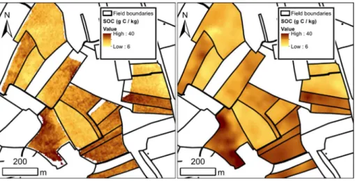
be observed anymore after land consolidation. SOC patterns in fields covering the hill slope from the crest to the foot slope showed patterns related to erosion of C associated with the topsoil. Stevens et al. (2015) further demonstrated the importance of land management on SOC content. Their residual maximum likelihood model (REML) applied to the SOC map produced from the AHS160 flight over Luxembourg predicted that a field effect accounted for 48 ± 8% of the variance in SOC content in a cluster of fields (Fig. 3).

The performance of the estimations obtained from regression models (MLR, PLSR, PSR, SVM…) is usually assessed with figures of merit such as the standard error of cali-bration, the standard error of prediction or the ratio of performance deviation, and these figures of merit evaluate the global model performance, as they are calculated during the model building and validation stages. A first evaluation of uncertainty that affects each prediction obtained by a hyperspectral airborne sensor has been realized by Gomez et al. (2015a). An evaluation of different types of uncertainties (i.e. variance of predictions) has been done: (1) prediction variance due to the regression model, (2) prediction variance due to the spectra and (3) prediction variance due to the interaction between these two effects, prediction variance due to differences between spectral predictors and spectral calibration samples. This paper showed that these prediction uncertainty maps may be used to better

Fig. 3 Predicted SOC maps (left) from the AHS 160 campaign in Luxembourg (Stevens et al. 2010) and (right) using a residual maximum likelihood model (Stevens et al. 2015)

characterize the quality of the soil properties mapping results, mask no-soil pixels and define the soil sampling and the calibration dataset.

3.2 Soil Moisture

Water is considered to be one of the most significant chromophores in the soil system (Idso et al. 1975; Stoner and Baumgardner 1981; Baumgardner et al. 1985; Hummel et al. 2001; Lobell and Asner 2002). Bowers and Hanks (1965) described the effect of soil moisture content on reflectance for the first time. The main effect is the decrease in reflectance with increasing soil moisture, and some spectral features are more affected than others. Dalal and Henry (1986) isolated the main differences in absorbance (log 1/reflectance) and found them to be related to the variation in the moisture contents used across the 1100–2500-nm SWIR spectral region. Bishop et al. (1994) show the features directly associated with the OH group in the water molecule (at 1400 and 1900 nm), and some are indirectly associ-ated with the strong OH group in the thermal infrared region (around 2750–3000 nm) that affect the lattice OH in clay (at 2200 nm) and CO3 in carbonates (at 2330 nm). Ben-Dor

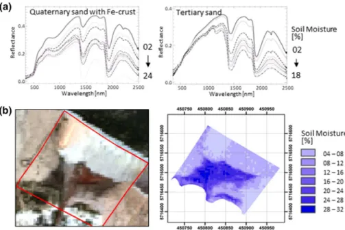
et al. (1999) have noted the diminishing of the 2200-nm absorption feature in Ca-mont-morillonite mineral at various relative humidity conditions. The highly sensitive 1900-nm region, a water OH combination band, showed an excellent nonlinear fit to the increase in water content. Muller and Decamps (2000) determined that the impact of soil moisture on reflectance could be greater than the differences in reflectance due to the soil categories, as it affects the baseline height (albedo) as well as several spectral features across the entire spectral range, as can be seen in Fig. 4a.

Fig. 4 a Influence of soil moisture on soil spectra from quaternary and tertiary sand; b determination of

gravimetric water content based on HyMap imagery: HyMap RGB image (left) and modelled gravimetric soil water content (in %) (right). Modified from Haubrock et al. (2008a, b)

Several studies focused on the modelling of soil spectral reflectance and soil water content. Bach and Mauser (1994) were able to simulate the reflectance change of the soil spectra from dry to moist through the use of various water film depths related to moisture content. They combined the model of Lekner and Dorf (1988) for internal reflectance with the absorption coefficients from Palmer and Williams (1974) into Lambert’s law (or Beer’s law) to simulate the moist reflectance R from the dry reflectance Ro by the exponential of the absorption coefficient and an empirically determined active thickness. They applied this process for predicting the water contents within an AVIRIS image of a partially irri-gated field and a dark organic soil field in the Freiburg test site in Germany from the image pixel spectra of dry and moist soils. The active thickness and water absorption coefficients predicted the amount of the soil’s water content to a high R2 _{of 0.88. Most recently, Bablet}

et al. (2018) have developed MARMIT, a multilayer radiative transfer model of soil reflec-tance to estimate soil water content that could be applied on imaging spectroscopy data in the laboratory, but not yet from remote sensing data.

Nowadays, robust spectral techniques to quantify and/or correct soil moisture content from surface reflectance exist that have been developed by several authors at the labora-tory level and tested successfully on hyperspectral imagery (e.g., Bryant et al. 2003; Whit-ing et al. 2004a, b; Haubrock et al. 2008a, b; Fabre et al. 2015; Diek et al. 2019). The approaches range from spectral indices, exponential or Gaussian models, to geostatistical models. Whiting et al. (2004a) fitted an inverted Gaussian function centred on the assigned fundamental water absorption region at 2800  nm, beyond the limit of commonly used instruments, over the logarithmic soil spectra continuum found with convex hull boundary points. The area of the inverted function, soil moisture Gaussian model (SMGM), accu-rately estimated the water content with coefficients of determinations (R2_{) of 0.94–0.98}

when samples were separated according to landform position (Spain) and salinity (USA). Using AVIRIS hyperspectral images of these soil regions in an air-dried status, they improved the abundance estimates of clay and carbonate abundance by 10% of the regres-sion mean by including the SMGM area as a parameter in the empirical determination (Whiting et al. 2005).

Haubrock et al. (2008a, b) developed a successful simple approach termed the Normal-ized Soil Moisture Index (NSMI) based on the edges of the water band centred at 1900 nm. It was developed in the laboratory and tested in the field for the best spectral prediction of soil moisture content taking into account the influence of different environmental factors, such as variable soil types, soil water profiles and the presence of soil crust and vegeta-tion cover; and in remote sensing data based on hyperspectral imagery. The NSMI allowed the production of surface soil moisture maps, generated from HyMap airborne images (Fig. 4b), which were found to be highly correlated with the field moisture content meas-ured at the time of the overflight (Haubrock et al. 2008b).

The NSMI and SMGM methods were successfully implemented in the soil mapping software tools HYSOMA and EnSoMAP (Chabrillat et al. 2011, 2016). Chabrillat et al. (2012) demonstrated that the two independent methods provide similar performances based on hyperspectral images for a same field, validated with ground data. Fabre et al. (2015) recognized that the water index soil (WISOIL) (Bryant et al. 2003) and the NSMI per-formed as good as the best soil moisture indices based on laboratory data. However, these indices are based on wavelengths located in or near the water absorption bands, which make them very sensitive to the quality of the atmospheric correction, and adapted indices were used by many authors (Fabre et al. 2015; Liu et al. 2003; Nocita et al. 2014). For that reason, Fabre et al. (2015), working on simulated spectral radiances at the sensor level, developed two additional soil moisture indices based on the wavelengths 2000–2200 nm

that are less sensitive to atmospheric correction, but more sensitive to variations in soil texture. The two indices are the normalized index of the NIR and SWIR domain for soil moisture content estimation from linear regression (NINSON) and the normalized index of the NIR and SWIR domain for soil moisture content estimation from nonlinear regression (NINSOL). Diek et al. (2019) present a first attempt to reduce the effect of soil moisture (SM) variation on reflectance data of soils, independent of new laboratory measurements. SM was determined by a newly developed SM index, similar to the existing NINSOL index, and was successfully applied to both field and airborne spectroscopy data, with R2 _of

0.75 and 0.59, respectively.

Nowadays, surface water content in soils can be cautiously estimated based on spectral reflectance, providing topsoil information that is not available at this scale through other systems and that could complement in bare areas the global estimates of near-surface soil moisture provided by microwave satellites. However, completely correcting the effect of soil water content on the reflectance mineral and organic band depths for an improved retrieval of other soil covariate continues to elude us. Further work in reconstructing the spectra will combine the spectral relationship of water content and soil components based on the physical nature of the materials and photon absorptions.

3.3 Soil Crust

Soil crust refers to a thin layer on top of the soil surface that is exposed to solar radiation and hence to the remote sensing sensors (Agassi et al. 1981). The arrangement of the upper thin layer of the soils, which actually formed the crust, is controlled by biogenic/organic process as well as by mechanical forces. Depending on the processes dominating the crust formation, soil crusts are termed biological/organic or physical. Biological/organic crusts are formed by communities of microorganisms that live on the soil surface, whereas physi-cal crusts are formed by physiphysi-cal impact such as that of raindrops.

Biological soil crusts, or biocrusts, are generated from live materials, such as complex communities of cyanobacteria, algae, lichen and mosses. Biocrusts modify the surface spectral response and can mask soil spectral properties (Weber et  al. 2008). For recent reviews on the effect of biocrusts on soil spectral signal and the biocrust mapping methods based on optical remote sensing, we refer to Escribano et al. (2017) and Weber and Hill (2016). In particular, it was shown that many studies referred to biocrust spectral traits at the laboratory and field scale, and approaches based on hyperspectral indices or spec-tral mixing analyses were developed to specspec-trally identify biocrusts or for biocrust surface cover quantification. For example, Weber et al. (2008) and Chamizo et al. (2012) developed two biocrust mapping hyperspectral indices that were used to map cyanobacteria-domi-nated biocrust in Soebatsfontein (South Africa) and in southern Spain, respectively, based on hyperspectral imagery. With this, the subtle spectral differences between sparse vegeta-tion, bare soil and biocrust could be identified. Nevertheless, important classification errors were observed in heterogeneous areas where each pixel is covered by a mixture of semiarid vegetation, bare soil and biocrusts (Alonso et al., 2014). Similarly, Hill et al. (1999) and Rodríguez-Caballero et al. (2014) used spectral unmixing methods to successfully quan-tify the amount of biocrust coverage within a pixel based on hyperspectral imagery in the Nitzana region (Israel), and in El Cautivo area (Spain). Some issues were observed in dis-criminating biocrusts in the areas dominated by vegetation, and an improved discrimina-tion could be obtained by the prior definidiscrimina-tion of areas into different land units.

Karnieli et  al. (1999) demonstrated that cyanobacteria provide unique spectral features on sand dune at the Negev area in Israel just as decomposed OM, whereas Ben-Dor et al. (1997) demonstrated that the same fresh OM may hold different spec-tral fingerprints based on the decomposition stage at the laboratory level. One of the important organic crusts that affect hydraulic conductivity of the thin surface layer is the OM with hydrophobic characteristics. This crust dramatically diminishes the infil-tration rate of water to the soil profile and hence increases erosion and soil degrada-tion and loss. Recently Ben-Dor et  al. (2017) demonstrated a significant correladegrada-tion between reflectance properties of the soil crust measured in the field by using the Soil-PRO apparatus and hydrophobicity field values as measured by the water droplet pen-etration time (WDPT) method over orchards trees soils, by thus demonstrating a pos-sible application based on future IS data.

The soil physical crust mostly refers to the rearrangement of soil particles as a result of the raindrop energy which disintegrates soil aggregates into a microstructure where fine particles are exposed at the top surface facing the Sun, and coarser parti-cles are found in the soil profile. In general, the factors leading to the formation of the structural crust (raindrop energy driven) are a combination of the kinetic energy impact of raindrops and the level of stability of the soil aggregates (Agassi et al. 1981, 1985). The structural crust is generated within minutes and significantly reduces the soil infiltration rate (IR). The crust hydraulic conductivity (HC) is lowered by a few orders of magnitude compared to the underlying soil (McIntyre 1958; Benyamini and Unger 1984). As the structural crust affects physical properties of the soil and can be observed by significant colour changes on the soil’s surface, spectral information, and especially on the surface, may be an excellent tool to monitor its status. To that end, spectral differences observed in the structural crust demonstrated that the upper micro-structure is composed of fine texture with some significant increase of the clay frac-tion (Ben-Dor et  al. 2004). Whenever the HC of the crust is lower than the rainfall intensity, ponding, runoff and soil erosion will follow crust (Agassi et al. 1981, 1985). These processes may further change the upper soil surface properties as seen by hyper-spectral sensor pointing on erosion, deposition and sedimentation effect over the soil in question.

Monitoring the soil crust condition is essential for the proper management of soils, from both an agricultural and land degradation perspective, and much work toward this end was done using reflectance spectroscopy at the laboratory level. Several studies demonstrated that reflectance spectroscopy can provide a valuable method for assess-ing the condition of the soil crust and estimatassess-ing the related problem (Demattê et al. 2004; Goldshleger et al. 2001; De Jong 1992; Eshel and Levey 2004; Ben-Dor et al. 2004). More studies toward this direction by Goldshleger et al. (2002, 2004) and Ben-Dor et al. (2003) demonstrated that the reflectance properties of soils can be an indi-cator for temporal processes that evolve on the soil surface due to runoff and erosion that were driven by the physical crust formation, based on laboratory experiments. An ambitious and very interesting study to upscale the physical soil crust spectral proper-ties from the laboratory (rain simulator) to the field and to remote sensing was done by Ben-Dor et al. (2004). In this study, loess (agricultural) soils from Israel were exam-ined for the soil crust at the laboratory which was then applied to the AisaEAGLE sensor to generate a soil infiltration map on a pixel-by-pixel basis (Fig. 5). Validation in the field confirmed the results and suggested that this idea could be extrapolated to other areas in order to prevent soil degradation processes by water erosion.

3.4 Soil Erosion and Degradation

Soils are considered non-renewable resources which have a limited extent, are unequally distributed geographically, are affected by degradation due to inappropriate land man-agement and use, but are essential to terrestrial life and human well-being (Lal 2015). Adverse climatic conditions and inappropriate human activities on land use can lead to a loss of soil quality and as a consequence to degradation of soil properties (Stolte et al. 2016). Soil degradation is a change in the soil health status resulting in a diminished capacity of the ecosystem to provide goods and services for its beneficiaries (FAO and ITPS 2015). Degraded soils do not provide services according to their original poten-tial in an ecosystem. Soil erosion, salinization, desertification and pollution are some of the main processes affecting soil degradation, which occur over space and time. Soil erosion is a land degradation process which is often found in cultivated environ-ments due to natural processes (e.g., climate events) and accelerated by human activi-ties (e.g., extensive tillage). Tillage-induced soil erosion brings about the progressive removal of soil horizons and the corresponding accumulation of soil materials at the slope (Previtali 2014). Furthermore, soil erosion may reduce crop production potential, lower surface water quality and damage tile drainage systems (Toy et al. 2002). Ero-sion is associated with about 85% of land degradation in the world, causing up to a 17% reduction in crop productivity (Oldeman et al. 1990). In Europe, soil loss is estimated at 2.46 t ha−1 _year−1 _{with a total loss of 970 Mt annually within agricultural, forests and}

semi-natural areas that are most affected by erosion (Panagos et al. 2015). To counteract land degradation, improvements are needed in methods of managing and monitoring of

Fig. 5 Mapping of soil infiltration on a pixel-by-pixel basis derived from AisaEAGLE hyperspectral imagery (after Ben-Dor et al. 2004)

soil resources (Eswaran et al. 2001). Mapping the extent of degraded lands and monitor-ing the situation in erosion-threatened soils are important in order to achieve the sus-tainable development goals set out by the United Nations. This implies sussus-tainable man-agement practices, soil conservation, restoration of degraded soils and improved land management practices (Ussiri and Lal 2018).

Remote sensing technologies can provide the necessary information for carrying out the assessment and monitoring of soil degradation processes such as soil erosion (Shoshany et al. 2013). Within the Vis–NIR and SWIR spectral regions, inorganic and organic components such as clay minerals, soil organic matter (SOM), iron oxides or calcium carbonate (CaCO3)

interact with the electromagnetic radiation and produce characteristic absorption features in soil reflectance spectra that can be used to identify soil properties when soils are exposed at the surface and vegetation cover is low (Chabrillat et al. 2002; Nanni and Demattê 2006; Ste-vens et al. 2013). Hyperspectral Vis–NIR–SWIR imaging has proven to be a promising tool to characterize and map topsoil properties (Chabrillat et al. 2002; Stevens et al. 2013; Schmid et al. 2016). This is especially relevant within Mediterranean regions where the exposure of bare-soil surfaces is common due to sparse vegetation cover and management practices such as leaving fields fallow (Bartholomeus et al. 2007; Gómez et al. 2012). Nowadays, it is well established that the quality of hyperspectral data is very important for quantitative assessment of key soil properties (Ben-Dor et al. 2009), and the soil properties determined by IS can be related to soil degradation processes. At present, there are a number of hyperspectral airborne sensors available worldwide such as HyMap (www.hyvis ta.com), HySpex (www.hyspe x.no) or Aisa (www.speci m.fi) that are suitable for soil studies. Furthermore, data from satellite-borne hyperspectral sensors such as Hyperion and CHRIS-PROBA exist and could be imple-mented to determine common soil properties such as clay minerals, iron oxide and calcium carbonate content. These two sensors were operating since 2000 and 2001, respectively, but the Hyperion sensor was decommissioned at the beginning of 2017. Then, as summarized in Sect. 1, there are a series of upcoming hyperspectral satellite-borne sensors that will be ideal for the monitoring of surface soil properties and related soil degradation.

Studies on soil properties and conditions have been carried out using data from field spec-troradiometer, hyperspectral and multispectral airborne and satellite-borne sensors to deter-mine the spatial distribution of surface soil properties and soil erosion on a local to regional scale (Ben-Dor et  al. 2006; Chabrillat 2006; Corbane et  al. 2008; Hill and Schütt 2000; Schmid et al. 2008; Vrieling et al. 2008). This approach is of interest when studying soil ero-sion as given in the example from Schmid et al. (2016). Here, hyperspectral data supported by morphological and physicochemical ground data were able to identify, define and map soil properties that could be used as indicators to assess soil erosion and accumulation stages (SEAS) in a Mediterranean rainfed cultivated region (Camarena, near Madrid, Spain). These properties were characterized by different soil horizons that emerge at the surface as a con-sequence of the intensity of the erosion processes, or the result of accumulation conditions. Therefore, selected sites representing different soil properties for the SEAS were used to train the SVM classifier to obtain their spatial distribution (Fig. 6).

4 Challenges and Gaps

There is a known decrease of soil properties’ prediction performances from laboratory to airborne imaging spectroscopy that has been demonstrated by several authors. This performance decrease is due to the combination of several effects such as differences in

the measurement conditions (sensors performances, different acquisition altitudes, opti-cal angles and lighting conditions), target structure and composition differences (labora-tory soil samples are dried, crushed and sieved while hyperspectral airborne targets are natural surfaces with heterogeneous surface temperatures and mixture in the field of view, moisture levels and roughness). The three main factors affecting the soil reflec-tance and so the model prediction accuracy have been assigned to (e.g., Stevens et al. 2008; Ben-Dor et al. 2009; Lagacherie et al. 2008): (1) the atmosphere; (2) a low signal-to-noise ratio of the imaging sensor data and (3) disruptive factors affecting the soil sur-face (partial vegetation cover, moisture, crust). Additionally, the availability of soil data, linked to the ad hoc need for calibration data, is a global challenge for the modelling of soil properties. Below, we present a summary of the main challenges and avenues of future research for global soil mapping and monitoring applications based on imaging spectroscopy data. They are grouped into three categories of challenges associated with different sensors, platforms, and reflectance data preprocessing, different surface condi-tions and different methodologies used for soil properties extraction.

Fig. 6 Mapping of soil erosion and degradation stages derived from AisaEAGLE and AisaHAWK hyper-spectral imagery. Modified from Schmid et al. (2016)

4.1 Sensors, Platforms and Reflectance Data Preprocessing

Imaging spectroscopy data in the Vis–NIR–SWIR may be acquired by three types of plat-forms: unmanned aerial vehicles (UAV), satellite, and airborne which is the most common. Hyperspectral cameras that can be mounted on UAV are of recent manufacture and cover only the VNIR spectral domain. Although SWIR cameras for UAVs still need to be opti-mized in terms of size and weight, and the auxiliary devices needed during flight have to be miniaturized, first models are just becoming available (e.g., HySpex Mjolnir S-620 from Norsk Elektro Optikk, NEO). The UAV low altitude allows a high spatial (< 50 cm) and temporal resolution which bears a very high potential for applications in precision agri-culture at the field scale, with cost-effective and flexible deployment capability regarding meteorological conditions. The performance of soil properties estimation by hyperspectral UAV sensors has still to be evaluated. A first initiative of soil mapping by a UAV platform focused on a VNIR multispectral UAV sensor for organic carbon content estimation and gave encouraging results (Aldana-Jague et al. 2016).

Only one hyperspectral satellite sensor covering the full Vis–NIR–SWIR has been in orbit from 2000 to early 2017, the Hyperion sensor aboard EO-1 satellite, which provided a spatial resolution of 30 m, a spectral resolution of 10 nm, a medium–low signal-to-noise ratio and a swath of 7.5 km (Folkman et al. 2001). Few studies were carried out on soil properties mapping by Hyperion data. Gomez et al. (2008a) and Lu et al. (2013) mapped SOC content with moderate performances using Hyperion data. Lu et al. (2013) mapped total phosphorus and pH with moderate performances, whereas the cation exchange capac-ity prediction exhibited low efficiency. More hyperspectral Vis–NIR–SWIR satellite sen-sors are planned to be launched within the next years, as already noted earlier in this paper, with high radiometric quality (higher signal-to-noise ratio). Below, we review the impact of several issues related to sensors and data preprocessing on soil properties mapping.

4.1.1 Impact of Spatial Resolution

Gomez et  al. (2015b) studied the sensitivity of the clay content prediction with respect to the degradation of the spatial resolution on hyperspectral Vis–NIR–SWIR airborne data. Their results showed that the spatial resolution impact on clay content mapping may depend on both the spatial structure of the studied soil property and the size of the studied fields in cultivated areas. In their study area characterized by small fields (around 0.56 ha) and strong spatial structure of clay due to short-scale successions of the parent material, clay mapping performances using hyperspectral data were accurate with an R2 _{of 0.74 at}

5 m resolution and 0.66 at 30 m resolution (Fig. 7). Therefore, even over small-scale agri-culture fields, the spatial resolution planned for future PRISMA, EnMAP, SHALOM and HypXIM (Lefèvre-Fonollosa et al. 2016) satellite sensors seems to be promising for clay content mapping.

4.1.2 Impact of Spectral Resolution

Using laboratory spectroscopic Vis–NIR–SWIR data, Castaldi et al. (2016) obtained accu-rate clay prediction performances using spectra with bandwidths from 10 to 160 nm. In addition, Adeline et al. (2017) obtained accurate clay prediction performances using labo-ratory spectra with bandwidths of up to 200 nm. Adeline et al. (2017) observed that (1)

soil properties with large and pronounced spectral features (e.g., iron) are only slightly impacted by a decrease in spectral resolution and (2) soil properties with no spectral fea-tures (e.g., pH) may be strongly impacted by a decrease in spectral resolution, and this impact may be reduced if these soil properties rely on the beneficial effects of correlations with soil properties and with spectral features (e.g., correlation between pH and iron).

4.1.3 Impact of Atmospheric Attenuation

Rectification of atmospheric attenuation is critical in the IS domain, since if it is not prop-erly done, it may influence the spectral signals that mistakenly can be assumed as part of the soil chromophores and increase noise in the signal. The issue of precise atmospheric correction has been studied by many researchers, and a combination of radiative transfer modelling and empirical methods is found to solve most of the past problems. In recent publications, the sensor radiometric instability problems as well as new and simple indica-tors to judge and correct systematic effects in airborne IS sensors have been developed by Brook and Ben-Dor (2014, 2015). Also, Gomez et al. (2015b) studied the sensitivity of the clay content prediction due to atmospheric effects on hyperspectral Vis–NIR–SWIR airborne data and simulated satellite data. They observed that when a correct compensation of atmosphere effects was performed using an inverse radiative transfer model, only slight differences were observed between clay content maps obtained using airborne imagery and simulated satellite imagery.

4.2 Soil Surface Conditions: Soil Moisture and Soil Roughness, Partial Vegetation Cover

Short-term variations in soil surface conditions due to meteorological conditions or land management practices such as ploughing and greening of the crop fields to prevent soil erosion have all an effect on soil reflectance. Soil reflectance decreases with increasing soil moisture and with increasing soil roughness, and nonlinear effects on soil spectral features are also observed. The increase in partial vegetation cover changes completely the shape of soil spectral reflectance. In turn, variations such as in soil moisture, soil surface roughness and vegetation cover have a strong impact on the quality and accuracy of the prediction

Fig. 7 Sensitivity of clay content prediction with respect to degradation of the spatial resolution on hyper-spectral Vis–NIR–SWIR airborne data. Extracted from Gomez et al. (2015b)