This is an author-deposited version published in:
http://oatao.univ-toulouse.fr/
Eprints ID: 9293
To link to this article: DOI: 10.1109/TSP.2013.2269048
URL:
http://dx.doi.org/10.1109/TSP.2013.2269048
To cite this version:
Besson, Olivier and Bidon, Stéphanie Adaptive processing
with signal contaminated training samples. (2013) IEEE Transactions on Signal
Processing, vol. 61 (n° 17). pp. 4318-4329. ISSN 1053-587X
O
pen
A
rchive
T
oulouse
A
rchive
O
uverte (
OATAO
)
OATAO is an open access repository that collects the work of Toulouse researchers and
makes it freely available over the web where possible.
Any correspondence concerning this service should be sent to the repository
administrator:
[email protected]
Adaptive Processing With Signal Contaminated
Training Samples
Olivier Besson, Senior Member, IEEE, and Stéphanie Bidon, Member, IEEE
Abstract—We consider the adaptive beamforming or adaptive detection problem in the case of signal contaminated training samples, i.e., when the latter may contain a signal-like component. Since this results in a significant degradation of the signal to interference and noise ratio at the output of the adaptive filter, we investigate a scheme to jointly detect the contaminated samples and subsequently take this information into account for estima-tion of the disturbance covariance matrix. Towards this end, a Bayesian model is proposed, parameterized by binary variables indicating the presence/absence of signal-like components in the training samples. These variables, together with the signal ampli-tudes and the disturbance covariance matrix are jointly estimated using a minimum mean-square error (MMSE) approach. Two strategies are proposed to implement the MMSE estimator. First, a stochastic Markov Chain Monte Carlo method is presented based on Gibbs sampling. Then a computationally more efficient scheme based on variational Bayesian analysis is proposed. Numerical simulations attest to the improvement achieved by this method compared to conventional methods such as diagonal loading. A successful application to real radar data is also presented.
Index Terms—Bayesian estimation, outliers, radar detection, ro-bust adaptive filtering.
I. PROBLEMSTATEMENT
O
PTIMAL multi-channel processing, either for beam-forming or detection purposes, requires the knowledge of the disturbance covariance matrix , so as to cancel out this disturbance and retrieve the signal of interest (SOI) with maximum signal to interference and noise (SINR) ratio [1]. In practical situations however, this covariance matrix is unknown and needs to be estimated from a set of training samples , . In an ideal situation, i.e., with independent and identically distributed samples sharing the same covariance matrix , Reed Mallet and Brennan in [2] showed that samples, where stands for the number of channels, are necessary for the average SINR of the adaptive processor to be within of the optimal SINR. This rate of convergence is a crucial parameter since, in manyThe authors are with the Department of Electronics, Optronics and Signal of Institut Supérieur de l’Aéronautique et de l’Espace (ISAE), University of Toulouse, ISAE, Toulouse, 31055 France (e-mail: [email protected]; [email protected]).
cases, the disturbance characteristics might vary, and hence it is highly desirable to converge with minimal . However the rate of convergence is sensitive to non-homogeneity among the training samples and the assumption that the training samples share a common covariance matrix is questionable in many situations [3]. Numerous factors can contribute to non-homo-geneity of the training samples, including clutter heteronon-homo-geneity (e.g., dense scattering environments, land-sea clutter interfaces, power level fluctuations among the various patches of clutter) or contamination of the training samples by signal-like com-ponents (e.g., in the case of multiple closely-spaced targets with approximately the same velocity) [4]. In this paper, we focus on the latter problem, i.e., the presence in the training samples of outliers with a signature close to that of the SOI. This phenomenon has a detrimental effect on the performance of the adaptive processor, even when a limited number of samples are contaminated [4]. In the latter reference, the probability of detection and probability of ghosting of Kelly’s generalized likelihood ratio test and the mean level adaptive detector are studied, in the case where only one sample out of is contaminated. Even with this small proportion of outliers, some degradation is observed. Note that if all training samples contain a signal component, the number of samples required for convergence of the adaptive processor is highly increased and is typically of the order [5], [6]. In fact, since the adaptive weight vector lies in a space orthogonal to that of the interferences, if a signal with the same signature as the SOI is present in the training samples, the adaptive filter is likely to place nulls towards the SOI, resulting in a significant SINR loss. The usual approach to cope with this problem is to select the most homogeneous set among the training sam-ples and to censor the other samsam-ples in the covariance matrix estimation procedure, see e.g., [7] for derivation of outliers resistant adaptive schemes. Very often, a test statistic is formed for each sample and compared to a threshold: only the samples whose test statistics do not exceed the threshold are retained. Several test statistics for detecting non-homogeneous samples have been proposed in the literature, e.g., power selection criteria [8], the generalized inner-product [9], the adaptive power residue [10] or the non-homogeneity detector [11]. Re-finements of these methods include a re-iterative censoring of the samples, see e.g., [10], [12], [13]. These methods perform well but may need a fairly large amount of initial data. In [14] an outlier-resistant adaptive beamforming scheme is proposed, which does not censor any sample. The author considers a compound-Gaussian model for the noise and the usual iterative scheme [15] which is known to converge to the maximum like-lihood estimate of the noise covariance matrix [16]. The idea
is to introduce diagonal loading within the iterations in order to obtain an improved robustness in the case where signal-like components contaminate the training samples.
In this paper, we also investigate an approach where all sam-ples are used but, at the same time, we try to detect whether a sample contains a signal-like component: if this is the case, the contribution of the latter to the training sample is somehow re-moved, but the concerned snapshot is not censored. Therefore, our approach consists of a joint signal detection-covariance ma-trix estimation scheme. Its principle relies on introducing bi-nary variables which indicate the presence or the absence of a signal-like component. These variables are assumed random and therefore a Bayesian framework is favored here, where both the presence indicators, the corresponding amplitudes and the covariance matrix are jointly estimated. All variables are as-signed some (non-informative) priors and the main contribution of the paper lies in deriving the minimum mean-square error (MMSE) estimator of under this framework. A Markov Chain Monte Carlo (MCMC) simulation method, based on Gibbs sam-pling, is first proposed. Then a computationally more efficient scheme, based on variational Bayesian (VB) analysis, is pre-sented.
II. MODELASSUMPTIONS
Let us assume that we have training samples which consist of noise and possibly a signal-like component, so that they can be modeled as
(1) where stands for the signature of the signal of interest and the following hypotheses are made.
The noise vectors are assumed to be independent, com-plex-valued Gaussian distributed, with zero-mean and covari-ance matrix , i.e.,
(2) As said previously, we adhere to a Bayesian framework and hence, we consider that is a random variable, with a conju-gate prior distribution relative to (2), namely an inverse Wishart distribution with mean and degrees of freedom, viz
(3) where means proportional to and stands for the ex-ponential of the trace of the matrix between braces.We con-sider a situation where no accurate information about is avail-able that would help to choose a specific . In fact, since it will amount to diagonal loading (see below), a method which is known to be robust against various mismatches, we will mostly consider the case in the sequel.
The complex amplitudes of the signal-like components in are assumed to be independent, and distributed according to a Bernouilli-Gaussian distribution:
(4)
As it will be more convenient, especially in the variational Bayesian analysis, we will use a statistically equivalent model for , namely where and are independent random variables. The binary variables indicate the presence or the absence of a signal-like component in the training samples. They follow a Bernoulli distribution, denoted
as , which is given by . The
amplitudes are independent complex-valued Gaussian dis-tributed random variables with zero mean and (known) variance
, i.e., . The distribution of
vector is denoted as .
In the sequel, we assume that the probability of contaminated samples is known. Extension to the case where is itself an unknown random variable with non informative uniform prior will be dealt with in the Appendix where we proceed to the generalization of the estimators derived below. Also, a sensi-tivity analysis will be conducted in Section V in order to assess the robustness of the estimators to a non perfect knowledge of . Accordingly, the extension to the case where is a random variable with non-informative prior will be investigated in the Appendix.
As stated in the introduction, our main objective is to obtain an estimate of –or directly an estimate of – so as to compute a filter . Towards this end, a systematic approach consists in deriving the minimum mean-square error (MMSE) estimator of , which entails computing the posterior mean of . Therefore, as a preliminary step, one needs to obtain
an expression for where . Under
the hypotheses made, the likelihood function is given by
(5)
where and if is
contami-nated and 0 otherwise. In the previous equation stands for the Hadamard (element-wise) product. Note that
where . In order to obtain ,
we use Bayes rule, viz and hence
first derive . Towards this end, we need to marginalize with respect to (w.r.t.) and . From (5) and using the fact that , it follows that
(6) Next, observing that
(7) we can write
(8) where we used the fact that
. The posterior distribution of only is finally obtained as
(9) The MMSE estimator is given by the posterior mean, i.e., . From inspection of (9), it does not seem possible to obtain a closed-form expression for the posterior mean. Moreover, generating samples drawn from and approximating the integral by an arithmetic mean is not feasible as the posterior distribution in (9) does not belong to any known class of distributions. Therefore, we investigate two different approaches namely Gibbs sampling and variational Bayesian analysis which work on the joint posterior distributions of , and . In addition to leading to tractable distributions, these approaches enable one to obtain estimates of and and hence to detect the contaminated samples together with their ampli-tudes. Thus they provide additional information compared to estimating only.
III. GIBBSSAMPLER
As evidenced in (9), does not lead to a closed-form expression for and it does not seem to be trivial to generate samples according to this distribution. Therefore, re-sorting to a Gibbs sampler appears to be a judicious way to pro-ceed [17], [18]. The principle of the Gibbs sampler is to succes-sively generate samples distributed according to the posterior distribution of one variable, conditioned on all other variables, as usually the conditional posterior distributions of each vari-able are easier to simulate. Doing so, it is known that the samples so generated will be asymptotically distributed according to the posterior distribution of each variable, so that, for instance, the MMSE estimator can be approximated by the arithmetic mean
of the set of samples drawn. In our case, this amounts to derive
, and . The starting point
of the derivation is the joint posterior distribution which, under the stated assumptions, is given by
(10) It is straightforward to infer that
(11) where we used the fact that . It follows that
(12) with
(13) Accordingly, (10) implies that
(14) and hence is Gaussian distributed
(15) with mean and covariance matrix
given by
(16a) (16b) Finally, let us consider the conditional posterior distribution of
:
(17) which is recognized as an inverse Wishart distribution [19] with
degrees of freedom and parameter matrix
TABLE I
GIBBSSAMPLER FORESTIMATION OF , AND
At this stage, it should be noted that both and depend on through its inverse . Note also that the optimal filter depends directly on . Therefore, it is more natural (and convenient) to work with the precision ma-trix rather than with the covariance mama-trix. Towards this end we need to derive the posterior distribution of , conditioned on
, and : from (17), this posterior distribution is given by (19) It is important to note that all three distributions in (12), (15) and (19) are well-known distributions and hence it will be rather straightforward to draw samples from them. Our Gibbs sampling scheme is summarized in Table I. Once the matrices are computed, the MMSE estimator of can be approximated as
(20) where stands for the number of burn-in iterations and is the effective number of iterations. The Gibbs sampler also allows to obtain an approximate maximum a poste-riori (MAP) estimator of , and by selecting the triplet which results in the maximum value of the joint posterior distribution.
IV. VARIATIONALBAYESIANANALYSIS
Despite its usually good performance, the Gibbs sampler may suffer from slow convergence, i.e., a large number of samples may be required for the Markov chain to converge and the sam-pler to provide accurate estimates. This results in an increased computational cost, a non desirable feature. In order to improve convergence speed, variational Bayesian methods have recently emerged [20]–[22]. Briefly stated, the essence of variational Bayesian analysis is to approximate the posterior distribution by a product of distributions, each one of the latter involving only some variables. More precisely, in our case the goal is to
approximate as
(21) One then seeks the individual distributions , and of (virtually) independent random variables , and such that the resulting joint distribution of , and is as close as possible to . Observe, that if this approximation is accurate, the MMSE estimator of say parameter vector is given
by . The approximation is obtained by
minimizing the Kullback-Leibler divergence between the two distributions, and it can be shown that the solution satisfies the following set of equations [20]
(22a) (22b) (22c) where the expectations should be understood w.r.t.
, e.g.,
However, the set of equations in (22) do not provide an ex-plicit solution since, for instance, depends on expecta-tions computed from and . A natural way to compute the distributions which satisfy (22) is thus to iterate between (22a), (22b), and (22c): each factor is updated with the current value of the other factors. More precisely, as will be-come clear shortly, the procedure amounts to update a few mo-ments of each distribution. To be specific, let us start with the joint posterior distribution of , and in (10). Using(22a), we have that (dropping the subscript in the expectation when only one variable is concerned and hence there is no ambiguity.)
(23) Therefore, it appears that the variables are independent Bernouilli distributed variables with
(24) Note that depends on the expected values of , and which are not known but will be updated in the
iter-ative procedure. We next proceed to the derivation of from (22b)
(25) The distribution in (25) is recognized as a Gaussian distribution with mean and covariance matrix given by
(26a) (26b) Again the parameters of this distribution depend on the expectations of and . Note also, that
, i.e., the are independent since the covari-ance matrix of is diagonal. In order to complete the analysis, we now derive the distribution of :
(27) The above distribution is recognized as an inverse Wishart dis-tribution with degrees of freedom. The average value of
is thus, provided that ,
(28) The overall procedure using this variational approach is de-scribed in Table II.
V. NUMERICALILLUSTRATIONS
Performance of the Bayesian estimators is assessed first on synthetic data (application to real radar data will be presented in next section). We consider a radar scenario where
pulses, generated according to (1) and (2), are coherently
TABLE II
VARIATIONALBAYESIANMETHOD FORESTIMATION OF , AND
processed. The vector encompasses both thermal noise and clutter components. These two components are assumed to be mutually uncorrelated so that the covariance matrix is
where the subscript identifies the particular component. The thermal noise is assumed to be temporally white with power so that while the clutter signal is correlated from pulse to pulse. Its spectrum is assumed located around the zero-Doppler with a Gaussian shape such that the
th element of the covariance matrix is given by (29) where is the spectrum variance. The factor of pro-portionality in (29) is chosen to obtain a desired value for the clutter-to-noise ratio (CNR) defined as
In all simulations we set . We would
like to emphasize the fact that the covariance matrix
is not drawn from its prior distribution in (3). range gates are used to estimate the covariance matrix while of them are contaminated in the direction under test where is the Doppler frequency of the contamination. For each contaminated cell , the contamination level is monitored by the signal-to-noise-ratio defined as
Unless otherwise stated, in the simulations. As stated earlier in Section II, the prior matrix is chosen so as to regularize the covariance matrix estimation problem, i.e., . The numerical value of the factor is chosen as for conventional diagonal loading [23], i.e., . Note that this choice may not be optimal in the present case but, since the optimal loading level is scenario dependent and hard to find, we will resort to this usual rule of thumb. On the other hand, to choose the degree of a priori , observe from (17) that the mean
of when is
(30) The degree of a priori is then fixed to to ensure that the weight given respectively to the observations and to
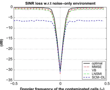
Fig. 1. SINR-loss versus Doppler frequency of the contaminated cells.
, , , .
in (30) is tantamount to a conventional diagonal loading. Inten-sive numerical simulations have demonstrated that many itera-tions are necessary to obtain an appropriate MMSE-estimation ( and ) whereas only a few iterations
are required for the VB algorithm to converge. The performance of the beamformers based on the Bayesian estimators (20) and(28) is assessed through the SINR-loss with respect to the noise-only-environment defined by [24]
where and denotes one of the estimates de-rived above. In addition to the MMSE- and VB-based formers, performance are also shown for the optimal beam-former , the conventional DL beamformer [23], [25] and the LNSMI beamformer [14]. For the latter the number of iterations used was and the loading level was chosen as in [14], i.e., times the largest eigenvalue of the sample covariance matrix of the normalized snapshots. Observe that, unlike conventional methods, the Bayesian algorithms of Table I and Table II also bring important information about the level of contamination for each range cell of the training in-terval.
We first consider an ideal situation where both the assumed level of contamination and the target power match perfectly the values used to generate the data. Fig. 1
displays the result in the case , and
. The influence of the number of secondary data is assessed in Fig. 2 where is increased to while the number of contaminated cells is kept to . In con-trast, we study in Fig. 3 the influence of which is increased to while . Finally, Fig. 4 investigates the influence of the power of the signal in the contaminated cells. Inspection of these 4 figures enables one to draw the following prominent properties of the various beamformers:
• The MMSE beamformer clearly outperforms the VB as well as the LNSMI, especially in low number of samples
Fig. 2. SINR-loss versus Doppler frequency of the contaminated cells.
, , , .
Fig. 3. SINR-loss versus Doppler frequency of the contaminated cells.
, , , .
or high number of contaminated cells. For example, the improvement compared to VB is, in the thermal noise
do-main, about for and about
for . Only in the case
(Fig. 2) do the VB and LNSMI approximately perform as well as the MMSE: in this case the three methods are really close to optimal.
• The MMSE beamformer is nearly insensitive to variations in the number of contaminated cells in terms of SINR loss: it incurs a loss from in Fig. 1 to
in Fig. 3. Additionally, a variation of the signal power in the contaminated cells induces negligible differences for the SINR loss.
• VB and LNSMI yield close SINR losses at least when . When the number of contaminated cells in-creases (see Fig. 3), VB is seen to incur a less severe loss, about for VB against for LNSMI. In contrast, VB and LNSMI behave similarly when the signal power in the contaminated cells increases: however, they are less
Fig. 4. SINR-loss versus Doppler frequency of the contaminated cells.
, , , .
robust than MMSE as a loss is observed when
goes from to .
• All methods clearly outperform diagonal loading: the latter undergoes severe performance degradation when the number or the signal level of contaminated cells increases. This poor performance is due to the nature of the data itself, i.e., the presence of outliers, and not to the choice of the loading level. Indeed, through many simulations (not reported in this paper) with different loading levels we experimented that diagonal loading is not effective in the clutter region whatever the diagonal loading level. Hence, looking for an optimal loading level for the particular model considered herein is questionable and, moreover, a delicate issue.
Our second series of simulations deals with robustness
anal-ysis of the beamformers. In the previous simulations,
perfor-mance of our Bayesian estimators has been studied when the processing parameters have exactly the same values as those used for signal generation. We now introduce mismatches be-tween the parameters used for generation and processing. The analysis will show that, to a certain extent, our estimators are quite robust so that a non-perfect knowledge of the scenario pa-rameters does not appear to be critical for a practical implemen-tation.
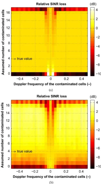
Figs. 5–6 study the influence of a mismatch in the assumed contamination level and in the assumed target power , respectively. In these figures, , , and we plot the SINR-loss resulting from this error with respect to the SINR-loss obtained without mismatch. The following observations can be made:
• Clearly the MMSE beamformer is almost not affected by a wrong assumption on or on .
• The VB appears to be more sensitive to both parameters. Interestingly enough, overestimating the number of con-taminated cells results in an improved SINR of the VB-es-timator, which then comes close to the MMSE estimator based on Gibbs sampling.
Fig. 5. Robustness towards a wrong assumption about the density of contami-nation . SINR-loss with respect to the Doppler frequency of the contaminated cells and the assumed number of contaminated cells. (a) MMSE estimation. (b) VB estimation.
Finally, to complete our robustness analysis, the effect of mismatch between the true direction of contamination and the direction under test is investigated. To do so, data are generated with a single direction of contamination and all the directions are tested. The SINR-loss so obtained is depicted in Fig. 7(a) when the contamination is near the clutter edge for and in Fig. 7(b) when the contamination oc-curs in the thermal noise domain for . For each beamformer presented, performance is affected only locally around the direction of contamination. The MMSE-beam-former endures only small losses in this region. Losses are more pronounced for both the VB- and LNSMI beamformer as they have naturally a lower SINR-loss than that of the MMSE in the true direction of contamination. Finally, the SCM-DL beamformer undergoes important losses in this region which may create a blind zone especially for a contamination near the clutter edge.
Fig. 6. Robustness towards a wrong assumption about the contaminating signal power. SINR-loss with respect to the Doppler frequency of the contaminated cells and the assumed contaminating signal power. (a) MMSE estimation. (b) VB estimation.
VI. EXPERIMENTALPARSAX RADARDATA
A. Experimental Setup
Performance of the Bayesian methods are now assessed on experimental data collected at the Delft University of Tech-nology on November 2010. Indeed, the International Research Centre for Telecommunications and Radar (IRCTR) has been developing these last years the polarimetric agile radar in S- and X-band (PARSAX) [27]. The system is situated on the rooftop of a 100m-high building and entails two reflector antennas, one to to transmit and one to receive. These two antennas can be con-sidered as colocated. The radar system has a flexible architecture with respect to the generated waveform and the pre-processing algorithms. For the experiment, a frequency modulated contin-uous waveform has been chosen as well as a deramping tech-nique for range compression. To assess the performance of our
Fig. 7. Robustness to steering vector mismatch. SINR-loss with respect to the desired Doppler frequency. (a) Doppler frequency of contaminated cells . (b) Doppler frequency of contaminated cells
.
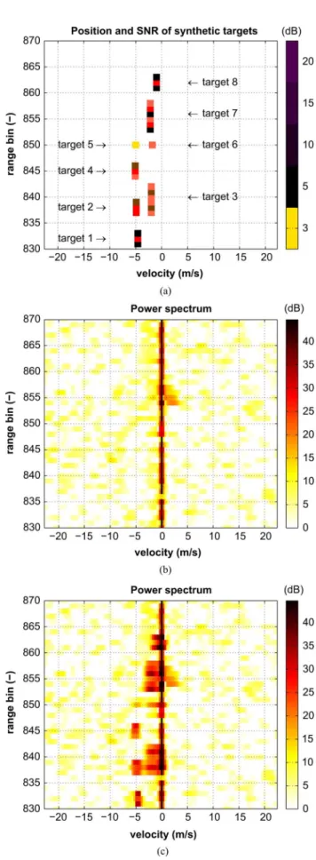
detectors, synthetic targets have been injected in a scene con-sisting mostly of a background noise and ground clutter. Loca-tion and SNR1of these targets are depicted on Fig. 6; they have
been chosen to reproduce a possible slow and heavy traffic. Note that given the range resolution, i.e., , a target may be extended in range. Other parameters describing the scenario are given in Table III. Note that we had at our dis-posal a data set containing only thermal noise (the antenna was pointed in the upward direction during a sunny day) so that the data are scaled to set the noise floor to 0 dB.
To give more insight into the scenario, the estimated power spectrum of the data to be processed is depicted in Fig. 8 before and after injecting the targets. As can be already observed, there is likely to be a true target around the range bin 855.
1To interpret more conveniently the next results, target amplitudes have not
been drawn randomly here but have been taken deterministically as .
TABLE III
PARSAX SCENARIOPARAMETERS
Given our robustness analysis we choose a high probability of contamination equal to and a contamination power equal to dB which is a compromise between the dif-ferent target powers. As the true covariance matrix is un-known, the SINR-loss can only be estimated, thus we prefer study hereafter the detection map obtained via the ACE [28] test statistic, i.e.,
(31) where is the cell under test. For each technique, the covariance matrix is estimated via a symmetric range-gate interval around the CUT with two guard cells. The ACE test statistic represents the angle between the target under test and the pri-mary data in the quasi-whitened space. It seems here to be a pertinent detector as it emerges as the solution to different de-tection problems [28]–[30], especially in non-homogeneous en-vironment.
B. Results
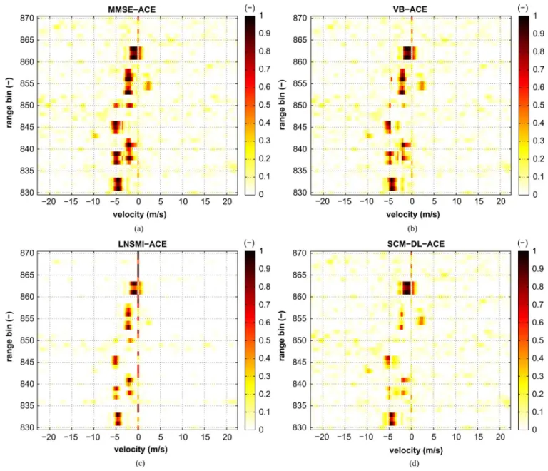
Detection maps obtained with the ACE detector (31) are de-picted in Fig. 9. The following comments can be made in accor-dance.
• Each target scatterer can be easily identified with the MMSE-ACE test statistic; even when the scatterer is near the clutter edge (targets 6 and 8) or when its power is low (targets 5 and 6). A few sidelobes are seen especially for target 8 near the clutter edge. Also, one can observe a slight clutter undernulling for a few range gates (e.g., around range bin 834 and 866).
• Same remarks can be made for the VB-ACE test statistic though a few more sidelobes can be seen (e.g., at range bins 831 and 833) and the scatterer peaks are somehow less pronounced. However, one has to keep in mind that the computational load of the VB algorithm is dramatically less than that of the MMSE-algorithm.
• The LSNMI-ACE misses some scatterers (e.g., within tar-gets 2 and 3 and target 5). However, these misses are com-pensated in a way by the absence of sidelobes (except for target 8 near the clutter edge) and a lower floor in the thermal noise domain. Note that the LNSMI-ACE is in-clined to a great clutter undernulling.
• The SCM-DL-ACE test statistic has the poorest perfor-mance which is in accordance with the prior study based on synthetic data. A lot of scatterers are missed (e.g., within targets 2, 3, 7 and the two low power targets 5 and 6). Before concluding our study, a last remark can be made about the possible targets that might be naturally in the data. Indeed,
Fig. 8. Range-velocity maps describing the data. (a) Location and SNR of the injected synthetic targets. Power spectrum via a 1D-APES filter [26] (b) prior to target injection (c) after target injection.
the previously mentioned true target at range bin 855 has been clearly identified by both the MMSE-, VB- and SCM-DL-ACE
Fig. 9. Range-velocity map. ACE-like detectors.
detectors. Also, the same detectors identify a target at range 843 which could not clearly be seen on the power spectrum map of Fig. 8. Note that the LNSMI-ACE detector misses both of them.
VII. CONCLUSIONS
In this paper, we considered the adaptive filtering problem in the case where some training samples are possibly contam-inated by signal-like components. This practically relevant situation, which is very detrimental to conventional adaptive filters, was addressed using a Bayesian approach where the variables indicating the presence of contaminated cells were assumed to follow a Bernoulli-Gaussian distribution. A non-in-formative prior was assumed for the noise covariance matrix, which helped regularize the covariance matrix estimation problem. Within this framework, the MMSE estimator was derived and implemented using a Gibbs sampler. A computa-tionally simpler scheme, based on variational Bayesian (VB) analysis was also proposed. The MMSE estimator was shown to come very close to the optimal adaptive filter, whatever the
proportion of contaminated samples or the power of the signal component in the training samples. Moreover, its robustness to non-perfect knowledge of these parameters was evidenced. The VB results in slightly increased SNR losses compared to the MMSE, yet at a much lower computational cost. Its implementation, as well as its performances, are comparable to those of the LNSMI. These algorithms were assessed against real radar data: in particular, the MMSE showed its ability to detect small targets close to the clutter ridge.
APPENDIX
EXTENSION TORANDOMHYPER-PARAMETERS In the main body of this paper, we assumed that and were known quantities and we carried out a sensitivity anal-ysis to assess the robustness of the various estimators to a non precise knowledge of these variables. An alternative option is to treat them as random variables with non-informative priors. In this appendix, we briefly indicate how the Gibbs sampling scheme and the variational Bayesian method can be extended to
the case of random hyper-parameters. More precisely, we now assume that is a random variable with uniform distribution on . Doing so we do not make any hypothesis about the probability of signal contamination and we estimate it jointly with the other parameters. Regarding we choose a conjugate inverse-Gamma prior distribution, denoted as , whose expression is
(32) Depending on the choice of and this prior can be made rather non informative. We now derive all necessary distributions to extend the estimators of the previous sections. For the sake of conciseness, we just provide the main steps since derivations are similar to those in the past sections. To begin with, the joint posterior distribution of all variables is now given by
(33)
A. Gibbs Sampler
It is straightforward to show that is still given by (11) and hence , conditioned on , , , and , is still Bernoulli distributed with the probability that it equals one still given by (13). Accordingly, the posterior distributions
and are the same as in
(14) and(17). The difference lies in the posterior distributions of and . As for , we have from (33) that
(34) which is a Beta distribution, i.e.,
(35) Finally, the conditional posterior of can be written as
(36)
and hence . The Gibbs
sampling scheme of Table I needs to be modified in order to account for the new variables which need to be generated.
B. Variational Bayesian Method
We now seek an approximation of the form
(37)
Using (33) along with derivations that led to(23), one can easily show that
(38) which implies that the variables are still independent Bernoulli distributed variables with mean value
(39) The derivation of leads to
(40) Hence is Gaussian distributed with mean and covariance matrix given by (26a)–(26b) except that should be substi-tuted for . Regarding it turns out that there is no modifica-tion compared to (27), and that has the same inverse Wishart distribution. Let us now consider :
(41) Therefore,
. As evidenced by (39), one needs to obtain the mean of and
which are given by [31, 4.253]
(42a) (42b) where is Euler’s psi function. Let us finally consider
:
which implies that . The mean value of is thus
(44) Again, the algorithm of Table II should be modified to update accordingly all new variables.
ACKNOWLEDGMENT
The authors would like to thank the IRCTR at TU-Delft for kindly providing the PARSAX experimental data.
REFERENCES
[1] L. L. Scharf, Statistical Signal Processing: Detection, Estimation and
Time Series Anal. Reading, MA, USA: Addison-Wesley, 1991.
[2] I. S. Reed, J. D. Mallett, and L. E. Brennan, “Rapid convergence rate in adaptive arrays,” IEEE Trans. Aerospace Electron. Syst., vol. 10, no. 6, pp. 853–863, Nov. 1974.
[3] W. L. Melvin, “Space-time adaptive radar performance in heteroge-neous clutter,” IEEE Trans. Aerosp. Electron. Syst., vol. 36, no. 2, pp. 621–633, Apr. 2000.
[4] K. Gerlach, “The effects of signal contamination on two adaptive detec-tors,” IEEE Trans. Aerosp. Electron. Syst., vol. 31, no. 1, pp. 297–309, Jan. 1995.
[5] D. M. Boroson, “Sample size considerations for adaptive arrays,” IEEE
Trans. Aerospace Electron. Syst., vol. 16, no. 4, pp. 446–451, Jul. 1980.
[6] H. L. Van Trees, Optimum Array Processing. New York, NY, USA: Wiley, 2002.
[7] K. Gerlach, “Outlier resistant adaptive matched filtering,” IEEE Trans.
Aerosp. Electron. Syst., vol. 38, no. 3, pp. 885–901, Jul. 2002.
[8] D. J. Rabideau and A. O. Steinhardt, “Improved adaptive clutter cancel-lation through data-adaptive training,” IEEE Trans. Aerosp. Electron.
Syst., vol. 35, no. 3, pp. 879–891, Jul. 1999.
[9] P. Chen, W. L. Melvin, and M. C. Wicks, “Screening among multi-variate normal data,” J. Multivar. Anal., vol. 69, no. 1, pp. 10–29, Apr. 1999.
[10] K. Gerlach, S. D. Blunt, and M. L. Picciolo, “Robust adaptive matched filtering using the Fracta algorithm,” IEEE Trans. Aerosp. Electron.
Syst., vol. 40, no. 3, pp. 929–945, Jul. 2004.
[11] M. Rangaswamy, “Statistical Anal. of the nonhomogeneity detector for non-Gaussian interference backgrounds,” IEEE Trans. Signal Process., vol. 53, no. 6, pp. 2101–2111, Jun. 2005.
[12] S. D. Blunt and K. Gerlach, “Efficient robust AMF using the Fracta al-gorithm,” IEEE Trans. Aerosp. Electron. Syst., vol. 41, no. 2, p. 537548, Apr. 2005.
[13] F. Lin, M. Rangaswamy, C. Wolfe, J. Chaves, and A. Krishnamurthy, “Three variants of an outlier removal algorithm for radar stap,” in
Proc. IEEE 4th SAM Workshop, Waltham, MA, Jul. 12–14, 2006, pp.
621–625.
[14] Y. I. Abramovich and N. K. Spencer, “Diagonally loaded normalised sample matrix inversion (LNSMI) for outlier-resistant adaptive fil-tering,” in Proc. ICASSP, Honolulu, Apr. 2007, pp. 1105–1108. [15] F. Gini and M. Greco, “Covariance matrix estimation for CFAR
detec-tion in correlated heavy tailed clutter,” Signal Process., vol. 82, no. 12, pp. 1847–1859, Dec. 2002.
[16] F. Pascal, Y. Chitour, J.-P. Ovarlez, P. Forster, and P. Larzabal, “Covariance structure maximum-likelihood estimates in compound Gaussian noise: Existence and algorithm Anal,” IEEE Trans. Signal
Process., vol. 56, no. 1, pp. 34–48, Jan. 2008.
[17] C. P. Robert and G. Casella, Monte Carlo Statistical Methods, 2nd ed. New York, NY, USA: Springer Verlag, 2004.
[18] C. P. Robert, The Bayesian Choice—From Decision-Theoretic
Foun-dations to Computational Implementation. New York, NY, USA:
Springer-Verlag, 2007.
[19] R. J. Muirhead, Aspects of Multivariate Statistical Theory. New York, NY, USA: Wiley, 1982.
[20] V.Šmídl and A. Quinn, The Variational Bayes Method in Signal
Pro-cessing. New York, NY, USA: Springer-Verlag, 2006.
[21] H. Attias, “A variational Bayesian framework for graphical models,” in Advances in Neural Inform. Processing Syst, S. A. Solla, T. K. Leen, and K.-R. Müller, Eds. Cambridge, MA, USA: MIT Press, 2000, pp. 209–215.
[22] M. J. Beal, “Variational algorithm for approximate Bayesian infer-ence,” Ph.D. dissertation, Univ. College London, London, U.K., 2003. [23] Y. I. Abramovich and A. I. Nevrev, “An Anal. of effectiveness of adap-tive maximization of the signal to noise ratio which utilizes the inver-sion of the estimated covariance matrix,” Radio Eng. Electron. Phys., vol. 26, pp. 67–74, Dec. 1981.
[24] J. Ward, “Space-time adaptive processing for airborne radar,”. Lex-ington, MA, USA, Lincoln Lab., MIT, Tech. Rep. 1015, Dec. 1994. [25] B. D. Carlson, “Covariance matrix estimation errors and diagonal
loading in adaptive arrays,” IEEE Trans. Aerosp. Electron. Syst., vol. 24, no. 4, pp. 397–401, Jul. 1988.
[26] J. Li and P. Stoica, “An adaptive filtering approach to spectral estima-tion and SAR imaging,” IEEE Trans. Signal Process., vol. 44, no. 6, pp. 1469–1484, Jun. 1996.
[27] O. A. Krasnov, G. P. Babur, Z. Wang, L. P. Ligthart, and F. van der Zwan, “Basics and first experiments demonstrating isolation improve-ments in the agile polarimetric FM-CW radar—PARSAX,” Int. J.
Mi-crow. Wireless Technol. (Special Issue), vol. 2, no. 3–4, pp. 419–428,
Aug. 2010.
[28] L. L. Scharf and L. T. McWhorter, “Adaptive matched subspace detectors and adaptive coherence estimators,” in Proc. Asilomar Conf.
Signals Syst. Comput., Pacific Grove, CA, USA, Nov. 1996, pp.
1114–1117.
[29] O. Besson, “Detection in the presence of surprise or undernulled inter-ference,” IEEE Signal Process. Lett., vol. 14, no. 5, pp. 352–354, May 2007.
[30] S. Bidon, O. Besson, and J.-Y. Tourneret, “The adaptive coherence es-timator is the generalized likelihood ratio test for a class of heteroge-neous environments,” IEEE Signal Process. Lett., vol. 15, pp. 281–284, 2008.
[31] I. S. Gradshteyn and I. M. Ryzhik, Table of Integrals, Series and
Prod-ucts, A. Jeffrey, Ed., 5 ed. New York, NY, USA: Academic, 1994.
Olivier Besson (SM’04) received the M.Sc. and Ph.D. degrees in signal processing in 1988 and 1992, respectively, from the Institut National Polytech-nique, Toulouse, France.
He is currently a Professor with the Department of Electronics, Optronics and Signal of ISAE (In-stitut Supérieur de l’Aéronautique et de l’Espace), Toulouse. His research interests are in the area of robust adaptive array processing, mainly for radar applications. Dr. Besson is a former Associate Editor of the IEEE Transactions Signal Processing and the IEEE Signal Processing Letters. He is a member of the Sensor Array and Multichannel technical committee (SAM TC) of the IEEE Signal Processing Society.
Stéphanie Bidon (M’08) received the engineer and master degrees from ENSICA, Toulouse, in 2004 and 2005 respectively and the Ph.D. degree from INP, Toulouse, in 2008.
She is now with the Department of Electronics, Optronics and Signal of ISAE (Institut Supérieur de l’Aéronautique et de l’Espace, Toulouse) as an assis-tant professor. Her research interests include digital signal processing particularly with application to air-borne radar.