To cite this document:
Jhinaoui, Ahmed and Mevel, Laurent and Morlier, Joseph
A CUSUM test with sliding reference for ground resonance monitoring. (2011)
In: The 6th International Workshop on Advanced Smart materials and Smart
Structures Technology (ANCRISST 2011 ), 25-26 Jul 2011, Dalian, China.
OATAO is an open access repository that collects the work of Toulouse researchers and makes it freely available over the web where possible.
This is an author-deposited version published in: http://oatao.univ-toulouse.fr/ Eprints ID: 6732
Any correspondence concerning this service should be sent to the repository administrator: staff-oatao@inp-toulouse.fr
The 6th International Workshop on Advanced Smart Materials and Smart Structures Technology ANCRiSST2011 July 25-26, 2011, Dalian, China
A CUSUM Test with Sliding Reference for Ground Resonance
Monitoring
Ahmed Jhinaoui
1and Laurent Mevel
INRIA, Centre Rennes- Bretagne Atlantique, Rennes 35042, France
Joseph Morlier
Université de Toulouse, ICA,
ISAE/INSA/UPS/ENSTIMAC, Toulouse 31055, France
ABSTRACT
Ground resonance is potentially destructive oscillations that may develop on helicopters rotors when the aircraft is on or near the ground. Therefore, this unstable phenomenon has to be detected before it occurs in order to be avoided by the pilot. To predict the zones of instability, works have generally relayed on off-line modal analysis of the helicopter model. Unfortunately, this off-line analysis is not sufficiently reliable. The subspace-based cumulative sum CUSUM test, able of on-line monitoring, is a good alternative which permits - at once- to avoid the system identification for each flight point and to have more robust detection, with reduced costs. In this paper, we describe an alternative test- with a moving reference this time- in order to kill wrong alarms or premature responses that are observed for fixed-reference tests. Numerical results reported herein are driven from simulation data.
INTRODUCTION
Ground resonance is a recurrent phenomenon of instability for helicopters. It is due to the coupling between the lagging motions of the rotor blades and the fuselage in-plane oscillations.
Since the works of Coleman and Feingold [1], in which a description of this phenomenon and a mechanical analysis were first given, numerous methods –analytic and numeric- have emerged and many papers have been published on the subject [2]. The main goal of these contributions was to give a sufficiently accurate mechanical modeling and, then, to determine the instability zone- that is the values of the rotor angular velocity at which the resonance may occur (i.e. the system is unstable when
one or more of the damping coefficients become negative). The disadvantage of this off-line and deterministic modal analysis is that it does not take into account the uncertainties for complex systems like helicopters. In fact, the dynamical behavior of this class of systems is function of much randomness (structural uncertainties, loads, erosion, fatigue…) so that the margins of stability could be affected [3]. The structure has, therefore, to be identified continuously in-flight and often tested on ground, which is costly in money and in time.
The subspace-based algorithm of detection offers an interesting alternative to deal with this problem. The main idea behind this method is to compute a criterion of instability at a stable reference and then, by some distance formula, determine when this distance is significantly different from zero. A comprehensive study of fault detection method can be found in [4,5].
A statistical cumulative sum (CUSUM) test [6] can be build for this subspace approach, in order to track eventual changes recursively i.e. in real-time. In previous works [7], the authors have investigated the capacities of this method to detect ground resonance. Results have shown that the test responds close to the instability but there still be a slight premature response before. This was predictable; the reference is taken far from the resonance region, so any slight change in the stability criterion (which is the value of the damping ratios) engenders a slight response of the test, and these responses are then cumulated in time, so that they could trigger a wrong alarm.
We describe herein an adaptive CUSUM test, which updates the reference recursively (sliding reference) and thus, kill all wrong responses. The paper is organized as follows: first, the principle of CUSUM subspace-based test is explained. Then, we give the analogous test for the case of sliding reference. Finally, both of two algorithms are applied to a simulation data of a helicopter with hinged-blades rotor.
SUBSPACE-BASED DETECTION WITH SLIDING REFERENCE
The subspace-based fault detection and isolation has enjoyed some popularity since its introduction in the seventies, and has found its application in many fields such as civil engineering and aeronautics. These methods are derived from the subspace-based identification which is reminded below, in its covariance-driven version. For more extended explanation, one can refer to [8].
Subspace Identification
Let consider the linear discrete system:
+
⋅
=
+
⋅
=
+ + k k k k k kv
x
H
y
w
x
F
x
1 1 (1)Wherex∈ℜnis the state vector,
F
∈
ℜ
nxnthe state transition matrix,H
∈
ℜ
rxnthe observation matrix andy∈ℜrthe output vector. The vectors wand vare two white Gaussian noises with zero means. The number of sensors r is chosen so that it is inferiorThe classical subspace identification method consists in building the Hankel matrix filled with the output covariances. Then, from a well-known factorization of this matrix into a product of the observability matrix and the controllability matrix, one can deduce the eigenstructure of the system in (1).
length of output data.
+ + + + = q p p p q q R R R R R R RR
R
L M O M M L L 2 1 1 3 2 2 1 cov H (2) Where Ri = E (yk yk-i T) is the correlation of the output data and E is the expectation operator. For a large number of data N, Ri could be estimated by
T i k N i k k i y y N R − + =
∑
= 1 1 . One can easily demonstrate that Hcovposses the factorization property:q p C O
Hcov = +1⋅ , with O and C, respectively, the observability and the Controllability matrices. And:
(3)
The subspace spanned by the left part of Hankel decomposition, namely the observability matrix, contains all the information about the eigenstructure of the system. This matrix can be obtained from a Singular Values Decomposition (SVD) ofHcov:
[
]
TV
U
U
Σ
Σ
=
0 1 0 1 covH
,O=U1Σ11/2 (4)Then, to extract the matrices of transition and observation F and H, a least square minimization is made:
O
O
F
=
, with = −1 p HF HF H M O , = p HF HF HF M 2 O (5)Once F and H found, the eigenvalues and the observed eigenvectors (λ, φλ) are computed by resolving
the equations: (6)
The couple (λ, φλ) is the eigenstructure of the system. It is stacked into the vector
vec
θ = Λ
Φ
where ᴧ
is the vector whose elements are the eigenvalues λi and Φ is the matrix whose columns are the mode shapes φi.
Subspace-Based Fault Detection
The fault detection consists in monitoring the eigenstructure and determining if any change
= + p p FH FH F M 1 O λ λ λ
ϕ
φ
φ
λ
I
F
I
H
F
−
)
=
0
,
(
−
λ
)
=
0
,
=
det(
has occurred on it. For that, a reference state θ0 and some distance, from this reference, called residual
are defined.
That distance is chosen as the product between a left kernel S of the matrix of observability (or ofHcov) at the reference, and this matrix at the current state θ: (
θ
0)⋅ p+1(θ
)T O S or ) ( ) (
θ
0 covp 1,qθ
T HS ⋅ + , S is taken so that ST.S=Id.
This distance is null when the current eigenstructure θ is close to θ0, and different from zero,
else. We build then the residual below [6]:
(7)
Where Yk+ =(ykT ... ykT+p)TandYk− =(ykT ... ykT−q+1)T and N the number of output data we have.
This residual is not useful for real-time detecting of instability on helicopters. First, because it is computed once one has all the N data. And second, because for an aircraft, the change on an eigenvalue does not mean that there is no more stability. In fact, the eigenvalues of a helicopter changes all the time with the rotor angular velocity; the helicopter is unstable when one of the damping ratios is negative. The residual we have should then be expressed as function of the damping coefficients ρi, and recursively for online detection.
) ) ( ( ) ( ) ( ) ( 0 0 1 0 − + − ⋅ ⋅ Σ ⋅ = k k T T k J vec S Y Y
Z
ρ
ρ
θ
θ
, J and Σ are the sensitivity and the covariance of theresidual. Consistent estimates of these matrices
∧
Jand
1 ^−
Σ
are given in [5].The CUSUM test to decide whether a change has occurred or no is (see [6,7] for more details):
The two hypotheses to test are
≈
0
:
0
:
) ( 1 ) ( 0 0 0f
ρ ρ n n g gE
H
E
H
(8)In order to have a response at the instability, the reference eigenstructure has to be taken close to the instable state. This is not possible for systems like helicopters, because it may lead to the destruction of the apparel. The reference is then taken far from resonance. In this case, any slight change in the damping would lead to a slight response of the test; these parasite responses are then cumulated and could trigger a false alarm. The modal analysis of a hinged blades helicopter given later in this paper will show that the damping ratios changes are not unimportant. So, the parasite responses would be significant.
CUSUM Test with Sliding Reference
The idea of tests with sliding reference derives from the adaptive algorithms which were investigated in some works [9,10,11]. These algorithms consist in subspace tracking by updating it,
) ) ( ( 1 )) ( ) ( ( 0 cov 0 kT p N q k k T T N vec S Y Y N H S vec N − − = +
∑
= ⋅ =θ
θ
θ
ζ
)
(
)
(
)
(
)
(
max
)
(
)
(
)
(
)
(
0 0 0 0 0 0 0 2 1 0ρ
ρ
ρ
ρ
ρ
ρ
θ
ρ
n n n k p n k q n k p n q k k nSum
T
g
Sum
T
Z
Sum
−
=
=
⋅
Σ
=
− ≤ ≤ − = −∑
using new coming data from sensors. The subspace which has to be tracked, in our case, is the left kernel S(θ0). This kernel is now computed for a sliding reference θn.
The recursive residual Zk writes this time: (9) ) ) ( ( ) ( ) ( ) ( k = T k ⋅Σ−1 k ⋅ T k ⋅ k+ k− k J vec S Y Y Z
ρ
ρ
θ
θ
The kernel Sk is updated with the IV-PAST method that is investigated in [12,10] and is computed for
the sample k-l with k the current sample and l some time lag fixed by the user. The algorithm can be described as follows:
• Compute an initial kernel S0 for some data tail N, (yq …yN-p)
• Then with IV-PAST, if we have Sn,(computed for data y from sample L to sample q+n-l-p, L is the length of the sliding window) Sn+1 is computed
• Jn and Σn -1
are estimated as in the fixed-reference case but using Sn in calculus, for the current
sample n
• The test is applied to compare the sliding reference at n-l and the current state n
The two hypotheses to test are
≈
0
:
0
:
) ( 1 ) ( 0f
n n n n g gE
H
E
H
ρ ρ (10)The utility of this algorithm is shown below on the application to a helicopter simulation data. It indeed permits to kill any premature response, and only responds when the system becomes unstable.
HINGED BLADES HELICOPTER MODEL
We give herein the equations of motion for helicopter’s ground resonance and a modal analysis of stability. Further mechanical explanations could be found in [7].
The class of helicopters considered herein is the one with in-plane hinged blades rotors. The model below is known to be a sufficiently precise description for ground resonance studies [1].
Fig. 1. Helicopter’s mechanical model- 3 blades
The helicopter’s fuselage is considered to be a rigid body with mass M, attached to a flexible LG (landing gear) which is modeled by two springs Kx and Ky, and two viscous dampers Cx and Cy as
n n n k p n k q n k p n q k k n Sum T g Sum T Z Sum − = = ⋅ Σ = − ≤ ≤ − = −
∑
max 2 1illustrated in Fig. 1. The rotor spinning with a velocity ω, is articulated and the offset between the MR (main rotor) and each articulation is noted a. The blades are modeled by a concentrated mass m at a distance b of the articulation point. Torque stiffness and a viscous damping Kβ and Cβ are present into
each articulation. The moment of inertia around the articulation point is Iz
The degrees of freedom are the lateral displacements of the fuselage x and y, and the out-of-phase angles βk=1…Nb, with Nb the number of blades.
State Vector Model
Applying the theorem of Lagrange to this model, one can demonstrate that [7]:
0 ) Im( ) ( Re ) Im( ) ( Re ) Im( ) ( Re . . . . .. .. .. .. = ⋅ + ⋅ + ⋅
η
η
η
η
η
η
l y x K l y x D l y x Mr r r (11)Where z=x+iy and η the Coleman [1] coordinate, such that:
∑
− = + ⋅ = 1 0 ) 2 ( b b N k N k t i k b e N ib
β
ω πη
. The matrices Mr, Dr and Kr write:
+
+
+
+
=
2 20
0
0
0
0
0
0
0
b
I
m
m
b
I
m
m
m
N
M
m
m
N
M
m
M
z z b b r + − + = 2 2 2 2 ) ( 2 0 0 ) ( 2 0 0 0 0 0 0 0 0 b C b I m b I m b C N C N C D z z b y b x r β βω
ω
− − + − − − + = ) 1 ( 0 0 ) 1 ( 0 0 0 0 0 0 0 0 2 2 2 2 2 2 2 2 mb I b a m b K b C b C mb I b a m b K N K N K K z z b y b x rω
ω
ω
ω
β β β βLet
e
=
[
x
Ty
TRe
l
(
η
)
TIm(
η
)
T]
Tand
=
⋅e
e
Linear Parameter-Varying (LPV): ) ( ). ( ) ( . t X A t
X =
ω
, and for the equation of observationY
(
t
)
=
C
.
X
(
t
)
, where:
⋅
−
⋅
−
=
− − r r r rK
M
D
M
I
A
(
ω
)
0
1 1 , we chooseC
=
[I
0
]
. Sampling the system at some rate τ yields the equations:k k k k k k w X C Y v X F X + = + = + + . ). ( 1 1
ω
, v and w are Gaussian noises with zero mean, and F=eτA (12)
Modal Analysis
The criterion of instability here is the drop of one or more damping ratios ρi from positive
values to negative ones (ρi <0). Given the matrix A, the variation of these coefficients with the angular
velocity can be plotted. They are computed using the eigenvalues λi of A:
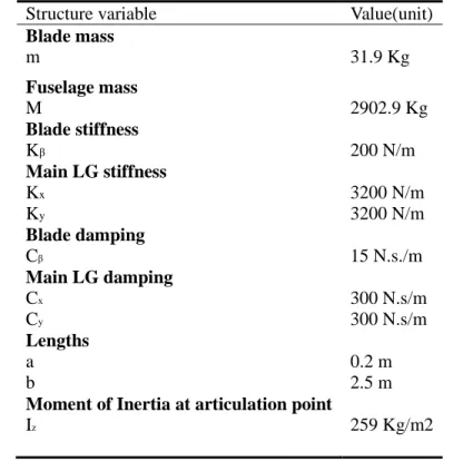
The plot is shown in Fig. 2 with the structural properties reported in Table 1.
Table 1. Structural properties for hinged-blades helicopter with 4 blades Structure variable Value(unit)
Blade mass m 31.9 Kg Fuselage mass M 2902.9 Kg Blade stiffness Kβ 200 N/m Main LG stiffness Kx Ky 3200 N/m 3200 N/m Blade damping Cβ Main LG damping Cx Cy 15 N.s./m 300 N.s/m 300 N.s/m Lengths a b 0.2 m 2.5 m
Moment of Inertia at articulation point
Iz 259 Kg/m2
Fig. 2 illustrates that the damping coefficients become positive and they are varying smoothly with rotor's angular velocity. The second modal damping coefficient ρ2 (mode 2) changes from
positive values to negative ones, from ω=1.62 rad/s to ω =2 rad/s, which is a criterion for ground resonance. It is this damping coefficient which will be monitored by CUSUM test.
A question to ask would be: why using the CUSUM test if we have the interval of instability from the modal analysis of the mechanical model? The answer is that this analysis is based on a
2 2 Im( ) ) ( Re ) ( Re i i i i l l λ λ λ ρ + − =
deterministic and off-line method and does not take that may affect the margins of stability. In
instability are highly sensitive to small changes flutter; the use of a statistical approach w
Fig. 2. Damping coefficients vs. blades angular velocity
Simulation Results for CUSUM Test
To test the performances of the sliding approach to the fixed model above is simulated at a rate τ
state of reference) to ω=2 rad/s by a step of 0.01 rad/s. For are simulated.
Fig. 3. Fixed reference CUSUM test response vs. sample
The fixed reference test responds for
zoom shows that the response occurs before. This was predictable
shown in Fig. 2) is continuously dropping; any change on its value engenders a response of the test. The response of the sliding test proves that, indeed, this approach kills any parasite response and the alarm is only triggered on near the instability, and not far from it.
CONCLUSION
The problem of detecting the ground resonance is addressed. An adaptive a
order to perform the response time and tested with simulation data. Future works encompasses a generalization of these methods to
anisotropic blades that leads to a
ACKNOWLEDGEMENTS
Zoom
method and does not take into consideration randomness
of stability. In [3] it is shown for the flutter phenomenon that airspeeds of highly sensitive to small changes in aircraft structure. Ground resonance is similar to
approach will then make the detection robust.
Fig. 2. Damping coefficients vs. blades angular velocity
Simulation Results for CUSUM Test
To test the performances of the sliding approach to the fixed-reference one, the helicopter model above is simulated at a rate τ=0.02 s. The angular velocity varies from ω=1 rad/s (taken as the =2 rad/s by a step of 0.01 rad/s. For each value of velocity, 1000 output samples
Fig. 3. Fixed reference CUSUM test response vs. sample
Fig. 4. Sliding reference CUSUM test response vs. sample
The fixed reference test responds for ω=1.6 rad/s, corresponding to the velocity of resonance, but a zoom shows that the response occurs before. This was predictable, the second damping coefficients, as shown in Fig. 2) is continuously dropping; any change on its value engenders a response of the test. response of the sliding test proves that, indeed, this approach kills any parasite response and the alarm is only triggered on near the instability, and not far from it.
The problem of detecting the ground resonance is addressed. An adaptive algorithm is proposed in order to perform the response time and tested with simulation data. Future works encompasses a generalization of these methods to a more complex model for helicopters rotors, which is the model of anisotropic blades that leads to a Linear Periodically Time-Varying system.
consideration randomness and uncertainties phenomenon that airspeeds of Ground resonance is similar to
reference one, the helicopter
ω=1 rad/s (taken as the
each value of velocity, 1000 output samples
Fig. 4. Sliding reference CUSUM test response vs. sample
corresponding to the velocity of resonance, but a , the second damping coefficients, as shown in Fig. 2) is continuously dropping; any change on its value engenders a response of the test. response of the sliding test proves that, indeed, this approach kills any parasite response and the
lgorithm is proposed in order to perform the response time and tested with simulation data. Future works encompasses a more complex model for helicopters rotors, which is the model of
This work was supported by the European project FP7-NMP CPIP 213968-2 IRIS.
REFERENCES
[1] R. P. Coleman and A. M. Feingold, "Theory of self-excited mechanical oscillations of helicopter rotors with hinged blades," NACA, Technical Report 1958.
[2] B. Eckert, "Analytical and a numerical ground resonance analysis of a conventionally articulated main rotor helicopter," Stellenbosch University, Thesis 2007.
[3] H. H. Khodaparast, J. E. Mottershead, and K. J. Badcock, "Propagation of structural uncertainty to linear aeroelastic stability," Computers and Structures, vol. 88, pp. 223-236, 2010.
[4] M. Basseville and I. Nikiforov, Detection of Abrupt Changes- Theory and Applications, Information and System Sciences Series ed. Englewood Cliffs, NJ: Prentice Hall, 1993.
[5] M. Basseville, M. Abdelghani, and A. Benveniste, "Subspace-based fault detection algorithms for vibration monitoring," Automatica, vol. 36, pp. 101-109, 2000.
[6] L. Mevel, M. Basseville, and A. Benveniste, "Fast in-flight detection of flutter onset : A statistical approach," AIAA Journal of Guidance, Control and Dynamics, vol. 28, no. 3, pp. 431-438, may 2005.
[7] A. Jhinaoui, L. Mevel, and J. Morlier, "Ground resonance monitoring for hinged-blades helicopters: statistical CUSUM approach," INRIA, Rennes, FR, 2010.
[8] P. Van Overschee and B. De Moor, Subspace Identification for Linear Systems, Theory,
Implementation, Applications.: Kluwer Academic Publishers, 1996.
[9] A. Benveniste, M. Metivier, and P. Priouret, Adaptive Algorithms and Stochastic Approximations.: Springer Verlag, 1990.
[10] I. Goethals, L. Mevel, A. Benveniste, and Bart De Moor, "Recursive Output Only Subspace Identification for In-flight Flutter Monitoring," in Proceedings of the 22nd International Modal
Analysis Conference (IMACXXII), 2004.
[11] R. Zouari, "An Adaptive Statistical Approach To Flutter Detection," in IFAC World Congress, Seoul, 2008, pp. 12024-12029.
[12] T. Gustafsson, "Instrumental variable subspace tracking using projection approximation," IEEE