HAL Id: hal-02369513
https://hal.archives-ouvertes.fr/hal-02369513
Submitted on 19 Nov 2019
HAL is a multi-disciplinary open access
archive for the deposit and dissemination of
sci-entific research documents, whether they are
pub-lished or not. The documents may come from
teaching and research institutions in France or
abroad, or from public or private research centers.
L’archive ouverte pluridisciplinaire HAL, est
destinée au dépôt et à la diffusion de documents
scientifiques de niveau recherche, publiés ou non,
émanant des établissements d’enseignement et de
recherche français ou étrangers, des laboratoires
publics ou privés.
A bi-objective robust inspection planning model in a
multi-stage serial production system
Mehrdad Mohammadi, Jean-Yves Dantan, Ali Siadat, Reza
Tavakkoli-Moghaddam
To cite this version:
Mehrdad Mohammadi, Jean-Yves Dantan, Ali Siadat, Reza Tavakkoli-Moghaddam. A bi-objective
robust inspection planning model in a multi-stage serial production system. International Journal of
Production Research, Taylor & Francis, 2017, 56 (4), pp.1432-1457. �hal-02369513�
A bi-objective robust inspection planning model in a
multi-stage serial production system
M. Mohammadi
a*, J.-Y. Dantan
b, A. Siadat
b, R. Tavakkoli-Moghaddam
ca
Ecole des Mines de Saint-Etienne, Department of Manufacturing Sciences and Logistics, CMP,
CNRS UMR 6158 LIMOS, 880 avenue de Mimet, 13541 Gardanne, France
b
LCFC, CER Metz - Arts et Métiers Paris Tech, Metz, France
c
School of Industrial Engineering, College of Engineering, University of Tehran, Tehran, Iran
Abstract
In this paper, a bi-objective mixed-integer linear programming (BOMILP) model for planning of an inspection process used to detect nonconforming products and malfunctioning processors in a multi-stage serial production system is presented. The model involves two inter-related decisions: 1) which quality characteristics need what kind of inspections (i.e., which-what decision) and 2) when the inspection of these characteristics should be performed (i.e., when decision). These decisions require a trade-off between the cost of manufacturing (i.e., production, inspection and scrap costs) and the customer satisfaction. Due to inevitable variations in the manufacturing systems, a global robust BOMILP (RBOMILP) is developed to tackle the inherent uncertainty of the concerned parameters (i.e., production and inspection times, errors type I and II, misadjustment and dispersion of the process). In order to optimally solve the presented RBOMILP model, a meta-heuristic algorithm, namely differential evolution (DE) algorithm, is combined with the Taguchi and Monte Carlo methods. The proposed model and solution algorithm are validated through a real industrial case from a leading automotive industry in France.
Keywords: Multi-stage production system; Conformity inspection; Monitoring inspection; Multi-objective
optimization; Robust optimization; Differential evolution.
1. Introduction
Since many production processes are technologically incapable of producing high-quality products, a quality management system (QMS) has gained increasingly high importance in many modern production systems, in which incapable production techniques, defective equipment and inferior raw materials are some of the external factors resulting in the quality problems. Accordingly, production managers are constantly attempting to provide a quality control system (QCS) to obtain high-quality products in the presence of such adverse external factors. In order to secure an effective QCS under such conditions, in-line quality control measures are employed more intensively, and if workable, automatically. For having an effective QCS, firms invest large amounts in inspection systems, and inspection planning problems stay on top of the manager’s concerns. Inspection allocation and selection decisions are actually made by quality managers; however, an overall framework for their decisions when they should decide which quality characteristics of the products need to be inspected and when to be inspected through the process and how to be inspected (i.e., which type of inspection) is almost missing.
Decisions regarding the inspection of products to detect the nonconforming parts before being sold are made in every production system. In particular, planning of inspection in a multi-stage production system (MPS), where raw materials are transformed into the final product through a series of distinct and consecutive processing stages has been recognized as one of the major necessities in production systems. Since the MPS presents various possibilities for inspection, inspection activities in the MPS may be performed after some or all of the processing steps. Therefore, inspection planning (IP) in the MPS is to determine the must-inspect quality characteristics as well as time and type of the inspections.
In the inspection planning process, conformity (CI) and monitoring (MI) inspections are integrated with production processes (Mohammadi et al., 2014a, 2015). CI is the collective term used for a number of activities (e.g., testing, inspection and certification) to specify whether the final product meets the designed characteristics. In other words, CI determines whether the product has been correctly manufactured based on the process plan and it complies with the design specifications. More importantly, in CI no deviation from the design specifications is allowed and the nonconforming products might be *Corresponding author. Tel: +33 2 29 00 10 30
reproduced or reworked in order to bring them into conformance. Therefore, the main aim of CI is minimizing the production cost by early detection of the nonconforming products as well as maximizing customer satisfaction through removing the defective products before being sold (Hinrichs, 2011; Etienne
et al., 2016). During CI, the production process is temporarily stopped and all products (i.e., 100%
frequency) or a sample of products are inspected to verify whether the most important quality characteristics meet the design specifications. Since stopping the production process results in a significant decrease in both yield and productivity, MI, with a lower frequency than CI, can be performed as a process status verifier, whereby critical processing features (e.g., feed speed of a drilling machine, force, temperature ant etc.) are monitored not to deviate from their set value.
Decisions regarding the implementation of CI and/or MI highly depend on the importance of the quality characteristics. For example, CI is implemented on quality characteristics, which directly correspond to the product function and even a small malfunction may highly decrease the customer satisfaction. On the other hand, MI is performed to increase the capability of the processes and to reduce the deviation from standard tolerances and ultimately, to minimize the number of defective/nonconforming products. Although simultaneous implementation of both CI and MI to secure quality characteristics is considered as the most reliable way to decrease the number of defectives and respectively reach the highest customer satisfaction level, due to recourse limitations, this consideration is mainly impractical as the total production cost would significantly be increased. Therefore, a trade-off between the production cost and customer satisfaction should be made to set the optimum inspection plan.
In addition to the elaborated concerns, lack of information about the production processes and several environmental factors impose a degree of uncertainty to the inspection planning decisions
(Galbraith, 1973; Ho, 1989). Although uncertainty and manufacturing variations (e.g., performance
degradation and non-conformance to specifications) are almost inevitable in practice, classical methods mainly consider deterministic conditions during the planning of an inspection process; while manufacturing processes are stochastic in nature. Consequently, a percent of the manufactured products do not conform the design specifications and the concerned process is sensitive to manufacturing variations. Traditionally, tight tolerance or higher precision manufacturing process was being applied to cope with this challenge, which mainly led to a huge manufacturing cost. Hence, manufacturers are interested in less sensitive manufacturing processes. These manufacturing processes are called robust processes that are relatively insensitive to alteration of uncertain parameters.
Finally, robust planning of an inspection process to pick out the critical quality characteristics and to determine the type and the location of the inspections is the main problem that this paper attempts to address.
The main contributions of this paper, which differentiate our efforts from those already published on the subject, are as follows:
Effectively integrating inspection plan with the production plan by performing inspection activities during the process instead of having an acceptance or a rejection check at the end. This integration minimizes the production cost by early detection of the nonconforming products.
Considering the monitoring inspection alongside the conformity inspection to monitor the processing parameters and avoid the creation of nonconforming products.
Proposing a new bi-objective mixed-integer linear programming (BOMILP) model for planning an inspection process.
Making trade-off between two important targets in almost all industries as manufacturing cost and customer satisfaction. These targets have been formulated as the objective functions of the proposed mathematical model.
Taking into account the uncertainty of the input parameters by developing a global robust approach based on the Taguchi loss function and the Monte Carlo simulation method.
Studying a real industrial case from a leading automotive industry in France to validate the performance of the proposed model and the robust solution approach.
Developing a tailored meta-heuristic algorithm, namely differential evolution (DE), to solve the real industrial case.
Investigating the sensitivity of the objective functions to the input parameters and extracting valuable managerial insights.
The rest of this paper is organized as follow. Section 2 reviews the relevant papers in the literature.
Section 3 explains the proposed BOMILP model. Section 4 describes the global robust optimization
approach. The solution algorithm is explained in Section 5. The experimental results of the real industrial case are provided in Section 6 and finally the paper is concluded in Section 7.
2. Literature review
Inspection planning problems have been studied by many researchers since the 1960s. Lindsay and
Bishop (1964) proposed a basic conceptual model and considered perfect inspection accuracy for
workstations of attribute data (WAD), in which all rejected items were scrapped. They also assumed that the inspection station could only check the outcome of the immediately preceding workstation. The extension of their study was proposed by White (1966) where the rejected items are replaced with conforming ones. Hurst (1973) first planned an inspection process by considering both type I and type II inspection errors. Peters and Williams (1984) provided five heuristic decision rules to find the location of the inspections. Later, Yum and McDowell (1987) extended the formulation of this problem in form of a mixed-integer linear programming model by adding the consideration of a rework activity. Chakravarty
and Shtub (1987) investigated the effect of setup and inventory carrying costs on the inspection strategy
(i.e., "all or none" versus partial inspection). They suggested a shortest path heuristic method to determine the strategic location of inspection activities and production lot sizes. Barad (1990) presented a solution-oriented technique based on the concept of break-even quality level. Viswanadham et al. (1996)
mathematically modeled the location problem of inspections in an MPS and developed two stochastic search algorithms for solving the problem, one based on simulated annealing (SA) and the other on genetic algorithm (GA). Their algorithms were developed to determine the location of the inspections resulting in a minimum expected total cost. Similarly, Bai and Yun (1996) constructed a cost model and a method for finding optimal locations of inspections and inspection level in an MPS. Lee and Unnikrishnan
(1998) developed a mathematical model in order to solve the inspection allocation and assignment
problems in an MPS, in which different part types with distinctive machine visitation sequences are processed and inspections can be performed on one of the several inspection stations with possible inspection errors. Verduzco et al. (2001) presented real-time inspection allocation that is based on the information gained by inspecting one additional component. They modeled the selection of which components to inspect as an information maximization problem. Besides, a modified knapsack greedy heuristic method was used to find near-optimal solutions to this optimization problem within the required time constraints. Regarding the integration of the production process and the inspection plan,
Lee and Kim (2001) proposed an optimization model to integrate the inspection planning and scheduling
using simulation-based genetic algorithms. The performance measures based on the process plan combinations calculated by a simulation module instead of process plan alternatives and the calculated measures are fed into a GA in order to improve the solution quality until the scheduling objectives are satisfied. Emmons and Rabinowitz (2002) studied the planning of the layout and operation of an inspection process used to detect malfunctioning processors in an MPS. Their planning involved three inter-related decisions: (i) the overall inspection capacity, (ii) the assignment of inspection activities to the inspectors and (iii) the scheduling of the inspector’s tasks. Kogan and Raz (2002) proposed a mathematical model of managing the intensity, sequence and timing of inspections in an N-stage production system with M inspection activities possible at each stage in order to minimize the sum of the inspection costs and the penalties caused by undetected defects. Shiau (2002, 2003a) studied the inspection resource assignment problem in a multi-stage manufacturing system by considering the inspection errors. They considered a limited number of inspections to be allocated through the production process. The author also considered the inspection errors that happen due to rapid changes of tolerances to satisfy the customer requirements.
Additionally, Shiau (2003b) studied inspection-allocation planning (IAP) problem for a multiple-characteristic manufacturing system, in which the production recourses are restricted and the limited number of inspections is considered for solving the IAP problem. This paper solved the IAP problem using a unit cost model, in which the manufacturing capability, the inspection capability, and specified tolerances are simultaneously considered. Rau and Chu (2005) considered inspection allocation problems for an MPS with two types of workstations, workstation of attribute data (WAD) and workstation of variable data (WVD), in which three strategies for the treatment of detected nonconforming units (i.e., repair, rework and scrap) were assumed. They developed a profit model for optimally allocating inspections and a heuristic solution method to solve the model. Hanne and Nickel (2005) developed a multi-objective inspection planning model considering objectives with respect to the quality (no. of defects), project makespan, and costs within a software development (SD) project. The developed model of SD processes includes different phases as coding, inspection, test, and rework and comprises the assignment of operations to the operators and the generation of a project schedule. Shiau et al. (2007)
integrated the production process and the inspection planning while higher performance of a production industry can be realized if the process and the inspection plans become integrated to cope with the limited manufacturing resources. They also developed a GA for solving large-sized problems. In a different work,
Ferreira et al. (2009) proposed an optimization model, in which decisions on determining the inspection intervals for MI under the failure of equipment and the decision maker preferences about the cost and the downtime are made simultaneously. Colledani and Tolio (2006) proposed an approach to evaluate the overall performance of a system considering both quality and production logistics. The results obtained by the application of the method provided new insight in the relations among the two areas and paved the way to the joint design of production logistics and quality control systems. In a similar work, Colledani and
Tolio (2012) presented a general theory to combine quality, maintenance and production control contexts
in an MPS in order to analyze the production rate of conforming products in the manufacturing systems with progressively deteriorating machines and preventive maintenance. In addition, due to the increasing pressure on high precision manufacturing and the development of on-line measurement technologies,
Colledani et al. (2014a) presented an integrated quality and production logistics model to profitably
manage the trade-off between selective and adaptive assembly systems in emerging sectors, such as micro-production, biomedical and e-mobility industry. In another work, Colledani et al. (2014b) proposed the production quality as a new paradigm aiming at going beyond traditional six-sigma approaches. Their new paradigm is extremely relevant in various technology intensive and emerging strategic manufacturing sectors. They claimed that the traditional six-sigma techniques show strong limitations in highly changeable production contexts, characterized by small batch productions, customized, or even one-of-a-kind products, and in-line product inspections. Therefore, innovative and integrated quality, production logistics and maintenance design, management and control methods as well as advanced technological enablers have a key role to achieve the overall production quality goal. Finally, they revised problems, methods and tools to support this paradigm. Mohammadi et al. (2014a) developed an optimization framework for process inspection planning of an MPS with multiple quality characteristics. They developed a single-objective mixed-integer mathematical programming model to minimize the sum of manufacturing and warranty costs. They also investigated the effect of uncertainty in misadjustment and attempted to provide a robust inspection plan.
Regarding the uncertainty in the input parameters, Kanyamibwa and Ord (2000) developed a form of the loss function considering the variability of a production process, the decision loss, and the costs of sampling and inspection. Specifically, they considered monitoring a production process, which may undergo continuous mean shift and variance deterioration during a production run. Kallgren et al. (2003)
reviewed the present status of the role of measurement uncertainty in conformity assessment. Macii et al.
(2003) studied a theoretical analysis aimed at estimating the growth in decisional risks due to both
random and systematic errors. Also, they provided some useful guidelines about how to choose the test uncertainty ratio of industry-rated measurement instruments in order to limit the risk of making wrong decisions below a maximum preset value. Pajula and Ritala (2006) illustrated through a case study, how the control a structure design that has been affected by uncertainty and how the corresponding dynamic problem is defined and solved with rather regular tools. The interested readers are referred to the recent review of impact of uncertainty in production inspection done by Desimoni and Brunetti (2011).
From the other aspect, some researchers have considered uncertainty in terms of risk in manufacturing processes. Bassetto et al. (2011) presented the concept of risk typology and its use in the management of process control deployment at a fab-wide level. They provided a comprehensive method based on the failure mode effect and criticality analysis (FMECA) to control failures that count throughout an organization. Khan and Haddara (2003) presented a new methodology for risk-based maintenance-inspection planning. They proposed a comprehensive and quantitative methodology that comprises three main modules; namely, risk estimation module, risk evaluation module and maintenance-inspection planning module.
Regardless of the context, several approaches have been developed to cope with the inherent uncertainty of the input parameters (see Zahiri et al., 2014a; Mousazadeh et al., 2015; Zahiri et al., 2015;
Rezaei-Malek et al., 2016; Zahiri et al., 2016; Zahiri and Pishvaee, 2016; Zahiri et al., 2017), out of which,
the robust design has been shown to be the most effective technique in manufacturing process to better address the manufacturing variations and uncertainty of the corresponding input parameters (Xiaoping and Chen 2000; Beiqing and Du, 2006; Hans-Georg and Sendho, 2007; Chen et al., 1996; Arvidsson and Gremyr, 2008; Torben et al., 2009; Gyung-Jin and Hee-Lee, 2002; Khalaj et al., 2012; Michael, 2013; Mechri
et al, 2014).
Almost all of the above-reviewed papers have only focused on allocating the inspection activities during the production process without considering other decisions such as picking out the critical quality characteristics to be inspected and selecting the type of inspection activities (i.e., MI and/or CI). Despite the literature, this paper integrates the inspection plan with the production process to simultaneously pick out the critical quality characteristics and to determine the type and the location of the inspections. Additionally, this paper takes into account the uncertainty of the input parameters and investigates the
effect of uncertainty on the final decisions. Comprehensively, this integration problem under uncertainty is presented as a new robust bi-objective MILP model with a trade-off between the production cost and the customer satisfaction as the two conflicting objective functions. There is no model in the literature that is able to effectively and efficiently address all of these challenges. The proposed model and the solution approaches are validated through a real industrial case study from one of the leading automotive industries in France. Finally, the sensitivity of the objective functions to the uncertain parameters is investigated to draw valuable managerial insights.
3. Problem description and mathematical formulation
This section, first, describes the problem and main decisions that need to made; and, second, develops the mathematical formulation based on a bi-objective mixed-integer linear programming model.
3.1. Problem description
Consider a serial MPS with N stages, in which an in-process part passes through stages 1 to N sequentially and inspections are performed at m stages where 𝑚 ≤ 𝑁. It should be noted that each stage can be an operation and a set of operations can be performed on the same machine. At each stage, a unique operation is performed on the part and a new quality characteristic is created in the part. The output of this stage is transferred to an inspection station or to the next processing stage. Suppose that a part consists of K quality characteristics and all these characteristics are created during the production process. A part is “nonconforming” if at least one quality characteristic does not meet the design specifications. If a CI is performed between stages i and i+1, there is an opportunity to detect the nonconforming parts originated from the ith stage or at some of the earlier stages. The detected nonconforming parts are scrapped and no further rework is allowed. On the other hand, if an MI is performed between stages i and i+1, the processing features are monitored after a specific number of parts. An inspection activity may involve two types of errors: misclassification of a conforming part as nonconforming (error type I) and nonconforming one as conforming (error type II).
This paper plans the inspection process through two main decisions as (1) which quality characteristics need what kind of CI or/and MI inspections (i.e., which-what decision) and (2) when the inspection of these characteristics should be performed (i.e., when decision). For the first decision, although those characteristics that have more impact on the product functionality and significantly affect the customer satisfaction should be picked out, but all the characteristics cannot be inspected while the inspection cost is highly increased. The second decision about the location of the inspections is also challenging, in which the inspection of a characteristic can be done just at special stages across the production process. For example, the process cannot be stopped or accessibility to and measuring that characteristic is impossible unless in some further stages. In addition, finding and removing nonconforming parts at initial stages is desired where nonconforming parts do not unnecessarily go through further operations and the cost of production is consequently decreased. Hence, it is more sensible to detect non-conformity immediately after its originating stage and before the next operation starts, but the number of inspection stations and the process interruptions as well as the total cost of inspection are increased. As an example, consider a situation that each characteristic is inspected immediately after its creation. Since each inspection activity includes three steps as: (1) removing the part from the machine, (2) inspecting and (3) setting up the part for the next operation; these steps are unnecessarily repeated for each characteristic. On the other hand, when a set of characteristics is inspected at a same allowable stage, the removing and setting up steps are needed only once. Therefore, making right and optimal which-what and when decisions are challenging and that this paper aims at coping with this challenge. Figure 1 shows the flowchart of the inspection planning decisions.
Figure 1. Inspection planning flowchart
3.2. Assumptions
The considered assumptions of the proposed BOMILP are listed as follows:
The production system contains N manufacturing stages arranged serially, wherein one part type is processed with K identical quality characteristics,
Different quality characteristics may be processed in a same manufacturing stage,
Non-conformities are generated only at the manufacturing processes and other activities such as movement, setup and inspection activities do not make non-conformity,
Each manufacturing stage has a failure rate of producing nonconforming parts,
Two types of conformity (CI) and monitoring (MI) inspections are considered, while considering MI for a manufacturing stage decreases the failure rate of that stage,
CI subjects to both errors type I and II, The frequency of MI is fixed,
MI affects the mean value of the process capability statistics such as Ppk,
Detected nonconforming items from CI are directly scrapped and no rework or repair operation is considered,
A unit scrap cost is imposed to the system in case of detecting a nonconforming part. The scrap cost depends on both the number of manufacturing stage and the quality characteristics,
The production system reaches a steady state and system breakdown is not assumed, Input parameters of the problem are considered to be uncertain,
In the robust model, we consider misadjustment that affects Cpk and Ppk as well as failure and scrap
rates.
3.3. Notations
Necessary notations for the proposed mathematical formulation are provided as follows:
Sets:
𝑝, 𝑝′∈ {1,2, … , 𝑃 + 1} Set of operations
𝑘 ∈ {1,2, … , 𝐾} Set of different quality characteristics
Parameters:
𝑓𝑟𝑝𝑘1 Failure rate of operation p for characteristic k with monitoring inspection
𝑓𝑟𝑝𝑘2 Failure rate of operation p for characteristic k without monitoring inspection
𝑑𝑝𝑘 Detection rate of conformity inspection assigned to operation p for characteristic k
𝛼𝑝𝑘 Type I error of conformity inspection assigned to operation p for characteristic k
𝛽𝑝𝑘 Type II error of conformity inspection assigned to operation p for characteristic k (𝛽𝑝𝑘= 1 −
𝑑𝑝𝑘)
𝑛𝑇 Total number of parts fed to the production process
𝑝𝑐𝑝 Unit production cost per time for operation p
n=1 n=i n=i+1 n=N Input Output Stage i m=1 m=i m=i+1 Stage i+1 If Q_Ch k needs inspection k=1
Select the Type of Inspection for k (CI/MI) Inspect the Q_Ch k Q_Ch k Conforms? Yes Nonconformity is negligable? No Yes Yes
Scrap the Part No If k<K k=k+1 Yes No Inspection Station Manufacturing Stage Q-Ch: Quality Characteristic No
𝑝𝑡𝑝 Production time of operation p
𝑠𝑐𝑝 Scrap cost of parts immediately after operation p
𝑛𝑐𝑘 Cost of nonconforming part in the market due to characteristic k
𝑓𝑚𝑝𝑘 Fixed cost of an MI station after operation p for characteristic k
𝑓𝑐𝑝𝑘 Fixed cost of a CI station after operation p for characteristic k
𝑣𝑚𝑝𝑘 Unit variable cost of MI per time performed after operation p for characteristic k
𝑣𝑐𝑝𝑘 Unit variable cost of CI per time performed after operation p for characteristic k
𝑚𝑡𝑝𝑘 Time of MI performed after operation p for characteristic k
𝑐𝑡𝑝𝑘 Time of CI performed after operation p for characteristic k
𝑓𝑠𝑝 Fixed space cost per part of establishing inspection stations just after operation p
𝜁𝑝′𝑝 Is 1 if two operations 𝑝′ and p are dependent; and 0, otherwise 𝜓𝑝𝑘 Is 1 if characteristic k belongs to operation p ;and 0, otherwise
𝑚𝑓𝑘 Monitoring frequency for characteristic k
𝑐𝑓𝑘 Conformity frequency for characteristic k
𝐺𝑘 Relative importance of characteristic k
M A big number
Decision Variables:
𝑁𝑃𝑝𝑘 Number of nonconforming parts due to characteristic k from operation p
𝑌𝐶𝑝𝑘 1 if operation p needs CI for characteristic k; and 0, otherwise
𝑌𝑀𝑝𝑘 1 if operation p needs MI for characteristic k; and 0, otherwise
𝑋𝐶𝑝𝑘′𝑝 1 if CI of operation 𝑝′ for characteristic k is performed immediately after operation p (𝑝′≤ 𝑝); and 0, otherwise
𝑋𝑀𝑝𝑘′𝑝 1 if MI of operation 𝑝′ for characteristic k is performed immediately after operation p (𝑝′≤ 𝑝); and 0, otherwise
𝑁𝑝 Number of parts entering operation p
𝑁𝑀𝑝𝑘 Number of MI performed between operations p and p+1 for characteristic k
𝑁𝐶𝑝𝑘 Number of CI performed between operations p and p+1 for characteristic k
𝑁𝑆𝑝 Is 1 if there is an inspection station between operations p and p+1
𝒮𝑝𝑘 Number of the scrapped part between operations p and p+1 due to characteristic k
𝑆𝑝 Total number of the scrapped parts between operations p and p+1
𝑂𝐹𝑉𝜏 𝜏th objective function value.
3.4. Mathematical formulation
This section develops the proposed BOMILP model by mathematically representing the which-what and when decisions. The first objective function of the model minimizes the total manufacturing cost which includes costs associated with production (TCP), scrap (TCS) and inspection (TCI). Total inspection cost contains total fixed inspection cost (TCIF) and total variable inspection cost (TCIV), where
TCI=TCIF+TCIV. The second objective function minimizes the customer satisfaction. Since customer
satisfaction is typically a qualitative factor, in this paper, minimizing the total warranty cost (TCW) is considered to capture customer satisfaction. Warranty cost is the cost when a nonconforming part reaches the customer and the company has to compensate the damages.
Through an inspection process plan, two different strategies can be adopted as well. First, a strategy considers that all characteristics need inspection and at most one kind of inspection (i.e., MI or CI) should be performed. Second, by relaxing some restrictions of the first strategy, it is considered that none, one or both of MI and CI (i.e., MI or/and CI) can be performed for each characteristic. Hereafter, the first and second strategies are called MI-or-CI and MI-and-CI strategies, respectively.
3.4.1. Objective functions
The objective functions of the model are mathematically formulated as Equations (1) and (2), respectively. Hereafter, the first and second objective functions are called as internal and external costs, respectively.
𝑂𝐹𝑉1= min{𝑇𝐶𝑃 + 𝑇𝐶𝑆 + 𝑇𝐶𝐼𝐹 + 𝑇𝐶𝐼𝑉} (1)
𝑂𝐹𝑉2= min{𝑇𝐶𝑊} (2)
𝑇𝐶𝑃 = ∑ 𝑝𝑐𝑝𝑝𝑡𝑝𝑁𝑝 𝑃 𝑝=1 (3) 𝑇𝐶𝑆 = ∑ 𝑠𝑐𝑝𝑆𝑝 𝑃 𝑝=1 (4) 𝑇𝐶𝐼𝐹 = ∑ ∑ 𝑓𝑐𝑝𝑘𝑁𝐶𝑝𝑘 𝐾 𝑘=1 𝑃 𝑝=1 + ∑ ∑ 𝑓𝑚𝑝𝑘𝑁𝑀𝑝𝑘 𝐾 𝑘=1 𝑃 𝑝=1 + ∑ 𝑓𝑠𝑝𝑁𝑆𝑝𝑁𝑝 𝑃 𝑝=1 (5) 𝑇𝐶𝐼𝑉 = ∑ ∑ 𝑐𝑓𝑘𝑐𝑡𝑝𝑘𝑣𝑐𝑝𝑘𝑁𝑝𝑋𝐶𝑝′𝑝 𝑘 𝐾 𝑘=1 𝑃 𝑝=1 + ∑ ∑ 𝑚𝑓𝑘𝑚𝑡𝑝𝑘𝑣𝑚𝑝𝑘𝑁𝑝𝑋𝑀𝑝′𝑝 𝑘 𝐾 𝑘=1 𝑃 𝑝=1 (6) 𝑇𝐶𝑊 = ∑ ∑ 𝐺𝑘𝑛𝑐𝑘(𝑁𝑃𝑝𝑘𝑌𝐶𝑝𝑘𝛽𝑝𝑘+ 𝑁𝑃𝑝𝑘× 𝑌𝑀𝑝𝑘) 𝐾 𝑘=1 𝑃 𝑝=1 (7) 3.4.2. Constraints
The constraints of the model have been provided as Constraints (8) to (18). ∑ 𝜁𝑝′𝑝𝑋𝐶𝑝𝑘′𝑝 𝑃 𝑝=𝑝′ = 𝜓𝑝′𝑘𝑌𝐶𝑝′𝑘 ∀𝑝′, 𝑘; 𝑝′≤ 𝑃 (8) ∑ 𝜁𝑝′𝑝𝑋𝑀𝑝𝑘′𝑝 𝑃 𝑝=𝑝′ = 𝜓𝑝′𝑘𝑌𝑀𝑝′𝑘 ∀𝑝′, 𝑘; 𝑝′≤ 𝑃 (9) 𝑌𝐶𝑝′𝑘+ 𝑌𝑀𝑝′𝑘 = 𝜓𝑝′𝑘 ∀𝑝′, 𝑘 (10) 𝑁𝑃𝑝𝑘= 𝑁𝑝× 𝑌𝑀𝑝𝑘𝑓𝑟𝑝𝑘1 + 𝑁𝑝× 𝑌𝐶𝑝𝑘𝑓𝑟𝑝𝑘2 ∀𝑝, 𝑘; 𝑝 ≤ 𝑃 (11) 𝒮𝑝𝑘≥ [𝑋𝐶𝑝′𝑝 𝑘 × 𝑁𝑃 𝑝′𝑘× 𝑑𝑝𝑘] + [𝑋𝐶𝑝𝑘′𝑝× 𝑁𝑝× 𝛼𝑝𝑘− 𝑋𝐶𝑝′𝑝 𝑘 × 𝑁𝑃 𝑝′𝑘× 𝛼𝑝𝑘] − [𝑋𝐶𝑝𝑘′𝑝× 𝑁𝑃𝑝′𝑘× 𝛽𝑝𝑘] ∀𝑝, 𝑝′, 𝑘; 𝑝, 𝑝′≤ 𝑃 (12) 𝑆𝑝≥ 𝒮𝑝𝑘 ∀𝑝, 𝑘; 𝑝 ≤ 𝑃 (13) 𝑁𝑝= 𝑁𝑝−1− 𝑆𝑝−1 ∀𝑝; 𝑝 ≤ 𝑃 + 1 (14) 𝑁0= 𝑛𝑇 (15) 𝑁𝑀𝑝𝑘≥ ∑ 𝑋𝑀𝑝′𝑝 𝑘 𝑃 𝑝′=1 ∀𝑝, 𝑘; 𝑝 ≤ 𝑃 (16) 𝑁𝐶𝑝𝑘≥ ∑ 𝑋𝐶𝑝′𝑝 𝑘 𝑃 𝑝′=1 ∀𝑝, 𝑘; 𝑝 ≤ 𝑃 (17) 𝑀 × 𝑁𝑆𝑝≥ ∑ ∑(𝑋𝐶𝑝′𝑝 𝑘 + 𝑋𝑀 𝑝′𝑝 𝑘 ) 𝐾 𝑘=1 𝑃 𝑝′=1 ∀𝑝, 𝑝′, 𝑘; 𝑝, 𝑝′≤ 𝑃 (18)
Equations (8) and (9) ensure that CI and MI of a quality characteristic should be done for all part just in one inspection stage, respectively. Equation (10) forces that one kind of inspection is needed for each quality characteristic. This equation is directly related to the MI-or-CI strategy. Equation (11) relates that the failure rate of an operation to the decision whether the MI is considered for that characteristic or not. Constraints (12) and (13) calculate the number of scraps after each inspection stage based on type I and type II errors. Constraints (14) and (15) determine the in-process part after each operation, where the number of parts is decreased in presence of any inspection due to scrap detection and removal. Equations (16) and (17) calculate total number of MIs and CIs throughout the whole production system. Constraint (18) calculates different inspection stage among the whole process.
3.4.3. Linearization
As it can be seen, the objective functions and some of the constraints include nonlinear terms and this issue makes the model difficult to solve. In order to address that, a linearization technique is applied to linearize the nonlinear terms. In this technique, the product of each pair of variables is replaced by a
new auxiliary variable and three extra constraints are added to the model for each pair. It must be noted that this technique is used when at least one of the variables is binary variable. For example, consider a binary variable X and a real variable Y. The problem is to linearize the product of these two variables (i.e., 𝑋 × 𝑌). Therefore, a new real auxiliary variable Z is considered. Next, the term 𝑋 × 𝑌 is replaced by Z in the whole model. Finally, the following three constraints should be added accordingly.
𝑍 ≤ 𝑀 × 𝑋, 𝑍 ≤ 𝑌,
𝑍 ≥ 𝑌 − 𝑀(1 − 𝑋).
Necessary auxiliary variables are provided as follows.
Auxiliary variables: 𝔸𝑝𝑘′𝑝 Linear form of 𝑋𝐶𝑝𝑘′𝑝× 𝑁𝑝′. 𝔹𝑝𝑘′𝑝 Linear form of 𝑋𝑀𝑝𝑘′𝑝× 𝑁𝑝′. 𝔻𝑝𝑘′𝑝 Linear form of 𝑋𝐶𝑝𝑘′𝑝× 𝑁𝑃𝑝′𝑘. 𝔼𝑝𝑘 Linear form of 𝑁𝑃𝑝𝑘× 𝑌𝐶𝑝𝑘. 𝔽𝑝𝑘 Linear form of 𝑁𝑃𝑝𝑘× 𝑌𝑀𝑝𝑘. 𝕃𝑝 Linear form of 𝑁𝑆𝑝× 𝑁𝑝. 𝕌𝑝𝑘 Linear form of 𝑁𝑝× 𝑌𝐶𝑝𝑘. 𝕍𝑝𝑘 Linear form of 𝑁𝑝× 𝑌𝑀𝑝𝑘.
3.4.4. The proposed BOMILP model under MI-or-CI strategy
After adding the linearization constraints (i.e., Constraints (23) to (46)), the final proposed BOMILP model under MI-or-CI strategy is proposed as follows.
BOMILP (MI-or-CI): min 𝑂𝐹𝑉1= ∑ 𝑝𝑐𝑝𝑝𝑡𝑝𝑁𝑝 𝑃 𝑝=1 + ∑ 𝑠𝑐𝑝𝑆𝑝 𝑃 𝑝=1 + ∑ ∑ 𝑓𝑐𝑝𝑘𝑁𝐶𝑝𝑘 𝐾 𝑘=1 𝑃 𝑝=1 + ∑ ∑ 𝑐𝑓𝑘𝑐𝑡𝑝𝑘𝑣𝑐𝑝𝑘𝔸𝑝 𝐾 𝑘=1 𝑃 𝑝=1 + ∑ ∑ 𝑓𝑚𝑝𝑘𝑁𝑀𝑝𝑘 𝐾 𝑘=1 𝑃 𝑝=1 + ∑ ∑ 𝑚𝑓𝑘𝑚𝑡𝑝𝑘𝑣𝑚𝑝𝑘𝔹𝑝 𝐾 𝑘=1 𝑃 𝑝=1 + ∑ 𝑓𝑠𝑝𝕃𝑝 𝑃 𝑝=1 (19) min 𝑂𝐹𝑉2= ∑ ∑𝐺𝑘𝑛𝑐𝑘(𝔼𝑝𝑘𝛽𝑝𝑘+𝔽𝑝𝑘) 𝐾 𝑘=1 𝑃 𝑝=1 (20) s.t.: (8)-(11), (13)-(18) 𝑁𝑃𝑝𝑘= 𝕍𝑝𝑘𝑓𝑟𝑝𝑘1 + 𝕌𝑝𝑘𝑓𝑟𝑝𝑘2 ∀𝑝, 𝑘; 𝑝 ≤ 𝑃 (21) 𝒮𝑝𝑘≥ [𝔻𝑝′𝑝 𝑘 × 𝑑 𝑝𝑘] + [𝔸𝑝′𝑝 𝑘 × 𝛼 𝑝𝑘− 𝔻𝑝′𝑝 𝑘 × 𝛼 𝑝𝑘] − [𝔻𝑝𝑘′𝑝× 𝛽𝑝𝑘] ∀𝑝, 𝑝′, 𝑘; 𝑝, 𝑝′≤ 𝑃 (22) 𝔸𝑝𝑘′𝑝≤ 𝑀 × 𝑋𝐶𝑝𝑘′𝑝 ∀𝑝, 𝑝′, 𝑘; 𝑝, 𝑝′≤ 𝑃 (23) 𝔸𝑝𝑘′𝑝≤ 𝑁𝑝′ ∀𝑝, 𝑝′, 𝑘; 𝑝, 𝑝′≤ 𝑃 (24) 𝔸𝑘𝑝′𝑝≥ 𝑁𝑝′− 𝑀(1 − 𝑋𝐶𝑝𝑘′𝑝) ∀𝑝, 𝑝′, 𝑘; 𝑝, 𝑝′≤ 𝑃 (25) 𝔹𝑝𝑘′𝑝≤ 𝑀 × 𝑋𝑀𝑝𝑘′𝑝 ∀𝑝, 𝑝′, 𝑘; 𝑝, 𝑝′≤ 𝑃 (26) 𝔹𝑝𝑘′𝑝≤ 𝑁𝑝′ ∀𝑝, 𝑝′, 𝑘; 𝑝, 𝑝′≤ 𝑃 (27) 𝔹𝑘𝑝′𝑝≥ 𝑁𝑝′− 𝑀(1 − 𝑋𝑀𝑝𝑘′𝑝) ∀𝑝, 𝑝′, 𝑘; 𝑝, 𝑝′≤ 𝑃 (28) 𝕍𝑝′𝑘 ≤ 𝑀 × 𝑌𝑀𝑝′𝑘 ∀𝑝, 𝑝′, 𝑘; 𝑝, 𝑝′≤ 𝑃 (29) 𝕍𝑝′𝑘 ≤ 𝑁𝑝′ ∀𝑝, 𝑝′, 𝑘; 𝑝, 𝑝′≤ 𝑃 (30) 𝕍𝑝′𝑘 ≥ 𝑁𝑝′− 𝑀(1 − 𝑌𝑀𝑝′𝑘) ∀𝑝, 𝑝′, 𝑘; 𝑝, 𝑝′≤ 𝑃 (31) 𝕌𝑝′𝑘≤ 𝑀 × 𝑌𝐶𝑝′𝑘 ∀𝑝, 𝑝′, 𝑘; 𝑝, 𝑝′≤ 𝑃 (32) 𝕌𝑝′𝑘≤ 𝑁𝑝′ ∀𝑝, 𝑝′, 𝑘; 𝑝, 𝑝′≤ 𝑃 (33) 𝕌𝑝′𝑘≥ 𝑁𝑝′− 𝑀(1 − 𝑌𝐶𝑝′𝑘) ∀𝑝, 𝑝′, 𝑘; 𝑝, 𝑝′≤ 𝑃 (34)
𝔻𝑝𝑘′𝑝≤ 𝑀 × 𝑋𝐶𝑝𝑘′𝑝 ∀𝑝, 𝑝′, 𝑘; 𝑝, 𝑝′≤ 𝑃 (35) 𝔻𝑝𝑘′𝑝≤ 𝑁𝑃𝑝′𝑘 ∀𝑝, 𝑝′, 𝑘; 𝑝, 𝑝′≤ 𝑃 (36) 𝔻𝑝𝑘′𝑝≥ 𝑁𝑃𝑝′𝑘− 𝑀(1 − 𝑋𝐶𝑝′𝑝 𝑘 ) ∀𝑝, 𝑝′, 𝑘; 𝑝, 𝑝′≤ 𝑃 (37) 𝔼𝑝′𝑘≤ 𝑀 × 𝑌𝐶𝑝′𝑘 ∀𝑝′, 𝑘; 𝑝′≤ 𝑃 (38) 𝔼𝑝′𝑘≤ 𝑁𝑃𝑝′𝑘 ∀𝑝′, 𝑘; 𝑝′≤ 𝑃 (39) 𝔼𝑝′𝑘≥ 𝑁𝑃𝑝′𝑘− 𝑀(1 − 𝑌𝐶𝑝′𝑘) ∀𝑝′, 𝑘; 𝑝′≤ 𝑃 (40) 𝔽𝑝′𝑘≤ 𝑀 × 𝑌𝑀𝑝′𝑘 ∀𝑝′, 𝑘; 𝑝′≤ 𝑃 (41) 𝔽𝑝′𝑘≤ 𝑁𝑃𝑝′𝑘 ∀𝑝′, 𝑘; 𝑝′≤ 𝑃 (42) 𝔽𝑝′𝑘≥ 𝑁𝑃𝑝′− 𝑀(1 − 𝑌𝑀𝑝′𝑘) ∀𝑝′, 𝑘; 𝑝′≤ 𝑃 (43) 𝕃𝑝≤ 𝑀 × 𝑁𝑆𝑝 ∀𝑝; 𝑝 ≤ 𝑃 (44) 𝕃𝑝≤ 𝑁𝑝 ∀𝑝; 𝑝 ≤ 𝑃 (45) 𝕃𝑝≥ 𝑁𝑝− 𝑀(1 − 𝑁𝑆𝑝) ∀𝑝; 𝑝 ≤ 𝑃 (46) 𝑋𝐶𝑝𝑘′𝑝, 𝑋𝑀𝑝𝑘′𝑝, 𝑁𝑆𝑝, 𝑌𝑝, 𝑌𝐶𝑝′𝑘, 𝑌𝑀𝑝′𝑘 ∈ {0,1} ∀𝑝, 𝑝′; 𝑝, 𝑝′≤ 𝑃 (47) 𝒮𝑝𝑘, 𝑆𝑝, 𝔻𝑝′𝑝 𝑘 , 𝑁𝑀 𝑝𝑘, 𝑁𝐶𝑝𝑘, 𝔸𝑝′𝑝 𝑘 , 𝔹 𝑝′𝑝 𝑘 , 𝑁𝑃 𝑝𝑘𝔼𝑝′𝑘, 𝔼𝑝′𝑘, 𝕃𝑝, 𝑁𝑝≥ 0 ∀𝑝′, 𝑝, 𝑘; 𝑝′, 𝑝 ≤ 𝑃 (48) where, Constraints (47) and (48) are domain constraint.
3.4.5. The proposed BOMILP model under MI-and-CI strategy
This section develops a BOMILP under the MI-and-CI strategy.
BOMILP (MI-and-CI): min 𝑂𝐹𝑉1= ∑ 𝑝𝑐𝑝𝑝𝑡𝑝𝑁𝑝 𝑃 𝑝=1 + ∑ 𝑠𝑐𝑝𝑆𝑝 𝑃 𝑝=1 + ∑ ∑ 𝑓𝑐𝑝𝑘𝑁𝐶𝑝𝑘 𝐾 𝑘=1 𝑃 𝑝=1 + ∑ ∑ 𝑐𝑓𝑘𝑐𝑡𝑝𝑘𝑣𝑐𝑝𝑘𝔸𝑝 𝐾 𝑘=1 𝑃 𝑝=1 + ∑ ∑ 𝑓𝑚𝑝𝑘𝑁𝑀𝑝𝑘 𝐾 𝑘=1 𝑃 𝑝=1 + ∑ ∑ 𝑚𝑓𝑘𝑚𝑡𝑝𝑘𝑣𝑚𝑝𝑘𝔹𝑝 𝐾 𝑘=1 𝑃 𝑝=1 + ∑ 𝑓𝑠𝑝𝕃𝑝 𝑃 𝑝=1 (19) min 𝑂𝐹𝑉2= ∑ ∑ 𝐺𝑘𝑛𝑐𝑘(𝔼𝑝𝑘𝛽𝑝𝑘+ 𝔽𝑝𝑘) 𝐾 𝑘=1 𝑃 𝑝=1 (20) s.t.: (8), (9), (11), (13)-(18), (21)-(48) 𝑌𝐶𝑝′𝑘+ 𝑌𝑀𝑝′𝑘 ≤ 2𝜓𝑝′𝑘 ∀𝑝′, 𝑘 (49)
4. Global robust optimization
As mentioned in Section 1, lack of information about production processes and several environmental factors imposes a degree of uncertainty to the planning parameters, which directly affect other decisions relating to the inspection process (Galbraith, 1973; Ho, 1989). In most of the manufacturing industries, a minimum level of uncertainty is inevitable. There are several parameters in the proposed BOMILP model that are affected by environmental factors and may fluctuate over the time. These parameters are production and inspection times, errors type I and II of the inspection activities, dispersion and misadjustment of the production processes. It should be noted that uncertainty in errors type I and II directly affects the number and cost of scraps and indirectly influences the warranty cost. In addition, uncertainty in dispersion and misadjustment of a process affects the failure rate and the number of scraps as depicted in Figures 2 and 3, respectively. Hence, manufacturers are interested in less sensitive manufacturing processes to the uncertain parameters. These manufacturing processes are called robust processes, which are relatively insensitive to alteration of the uncertain parameters. The main goal of this section is to take into account the uncertainty in the BOMILP’s parameters and to design a global robust BOMILP (RBOMILP) model.
L SL USL Mean Uncertain Dispersion Scrap Scrap Scrap Scrap
Figure 2. Uncertainty in dispersion
L SL USL Mean Misadjustment Scrap Scrap Mean Mean
Figure 3. Uncertainty in misadjustment
In order to design a robust inspection process, two methods have been proposed as follows (Das,
2000; Beyer et al., 2002):
Optimizing the expected value of the objective function under different alterations in the uncertain input parameters.
Minimizing the variance of the objective function under different alterations in the uncertain input parameters.
It is noteworthy that not only the expectation based measure does not sufficiently take care of fluctuations of the objective function while these fluctuations are symmetric around the average value, but also a purely variance based measure does not also take the absolute value of the solution into account. Hence, an optimization problem minimizing both expected value and variance of the objective function is desired to search the robust optimal solution. For these purposes, the Taguchi method is applied as the objective function (50) that should be minimized (Gyung-Jin et al., 2006). First, the necessary notations are provided below:
Parameters:
MCR Number of Monte Carlo runs
𝜔 Weight factor of standard deviation in the Taguchi method
𝐶𝑃𝑝 Process Capability. A simple and straightforward indicator of process capability
𝐶𝑃𝑘𝑝 Process Capability Index. Adjustment of CP for the effect of a non-centered distribution.
𝜌𝑀𝐼 Uncertainty factor of the process misadjustment under MI
𝜌𝐶𝐼 Uncertainty factor of process misadjustment under CI
𝜌σ Uncertainty factor of process dispersion
𝜌𝑇𝑃 Uncertainty factor of production time
𝜌𝑇𝑀𝐼 Uncertainty factor of MI time
𝜌𝑇𝐶𝐼 Uncertainty factor of CI time
𝜌𝑒_𝐼 Uncertainty factor of type I error
𝜌𝑒_𝐼𝐼 Uncertainty factor of type II error
Variables:
𝜇𝑂𝐹𝑉𝜏 Expected value of the 𝜏th objective function 𝜎𝑂𝐹𝑉𝜏 Standard deviation of the objective function 𝑅_𝑂𝐹𝑉𝜏 Robust value of the 𝜏th objective function
𝑅_𝑂𝐹𝑉𝜏 = 𝜇𝑂𝐹𝑉𝜏+ 𝜔𝜎𝑂𝐹𝑉𝜏 ∀𝜏 = 1,2 (50)
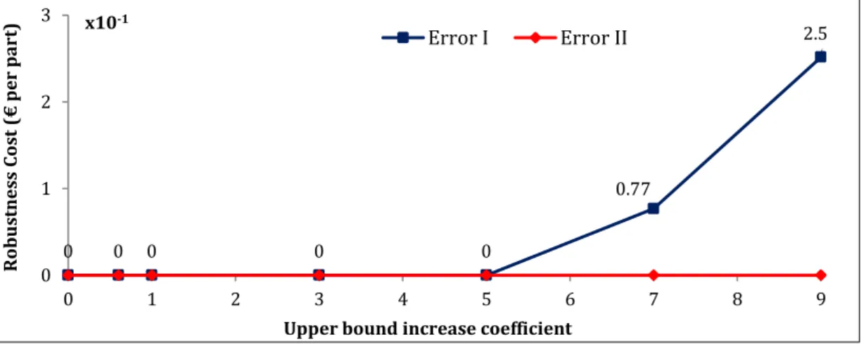
The alteration range for each uncertain parameter has been provided as Table 1.
Table 1. Alteration range of the uncertain parameters
Parameters Uniform alteration range
M is ad ju stm ent 𝑓𝑟𝑝𝑘𝑀𝐼 [⟦1 − 𝑃{𝑧 ≤ 3 × 𝐶𝑃𝑝} + 𝑃{𝑧 ≤ −3 × 𝐶𝑃𝑝}⟧, ⟦1 − 𝑃{𝑧 ≤ 3 × 𝐶𝑃𝑝− 𝜌𝑀𝐼} + 𝑃{𝑧 ≤ −3 × 𝐶𝑃𝑝− 𝜌𝑀𝐼}⟧] 𝑓𝑟𝑝𝑘𝐶𝐼 [⟦1 − 𝑃{𝑧 ≤ 3 × 𝐶𝑃𝐾𝑝} + 𝑃{𝑧 ≤ −3 × 𝐶𝑃𝐾𝑝}⟧, ⟦1 − 𝑃{𝑧 ≤ 3 × 𝐶𝑃𝐾𝑝− 𝜌𝐶𝐼} + 𝑃{𝑧 ≤ −3 × 𝐶𝑃𝐾𝑝− 𝜌𝐶𝐼}⟧] D is pe rs io n 𝑓𝑟𝑝𝑘𝑀𝐼 [⟦1 − 𝑃 {𝑧 ≤ 3 × 𝐶𝑃𝑝 1 − 𝜌σ } + 𝑃 {𝑧 ≤ −3 × 𝐶𝑃𝑝 1 − 𝜌σ }⟧ , ⟦1 − 𝑃 {𝑧 ≤ 3 × 𝐶𝑃𝑝 1 + 𝜌σ } + 𝑃 {𝑧 ≤ −3 × 𝐶𝑃𝑝 1 + 𝜌σ }⟧] 𝑓𝑟𝑝𝑘𝐶𝐼 [⟦1 − 𝑃 {𝑧 ≤ 3 × 𝐶𝑃𝐾𝑝 1 − 𝜌σ } + 𝑃 {𝑧 ≤ −3 ×𝐶𝑃𝐾𝑝 1 − 𝜌σ }⟧ , ⟦1 − 𝑃 {𝑧 ≤ 3 ×𝐶𝑃𝐾𝑝 1 + 𝜌σ } + 𝑃 {𝑧 ≤ −3 ×𝐶𝑃𝐾𝑝 1 + 𝜌σ }⟧] 𝑝𝑡𝑝 [𝑝𝑡𝑝(1 − 𝜌𝑇𝑃), 𝑝𝑡𝑝(1 + 𝜌𝑇𝑃)] 𝑚𝑡𝑝𝑘 [𝑚𝑡𝑝𝑘(1 − 𝜌𝑇𝑀𝐼), 𝑚𝑡𝑝𝑘(1 + 𝜌𝑇𝑀𝐼)] 𝑐𝑡𝑝𝑘 [𝑐𝑡𝑝𝑘(1 − 𝜌𝑇𝐶𝐼), 𝑐𝑡𝑝𝑘(1 + 𝜌𝑇𝐶𝐼)] 𝛼𝑝𝑘 [𝛼𝑝𝑘(1 − 𝜌𝑒−𝐼), 𝛼𝑝𝑘(1 + 𝜌𝑒−𝐼)] 𝛽𝑝𝑘 [𝛽𝑝𝑘(1 − 𝜌𝑒−𝐼𝐼), 𝛽𝑝𝑘(1 + 𝜌𝑒−𝐼𝐼)] M isa dju st m en t & D isp er sio n 𝑓𝑟𝑝𝑘𝑀𝐼 [⟦1 − 𝑃 {𝑧 ≤ 3 × 𝐶𝑃𝑝 1−𝜌σ} + 𝑃 {𝑧 ≤ −3 × 𝐶𝑃𝑝 1−𝜌σ}⟧ , ⟦1 − 𝑃 {𝑧 ≤ 3 × 𝐶𝑃𝑝 1+𝜌σ− 𝑟𝑀𝐼} + 𝑃 {𝑧 ≤ −3 × 𝐶𝑃𝑝 1+𝜌σ− 𝑟𝑀𝐼}⟧] 𝑓𝑟𝑝𝑘𝐶𝐼 [⟦1 − 𝑃 {𝑧 ≤ 3 × 𝐶𝑃𝐾𝑝 1−𝜌σ} + 𝑃 {𝑧 ≤ −3 × 𝐶𝑃𝐾𝑝 1−𝜌σ}⟧ , ⟦1 − 𝑃 {𝑧 ≤ 3 × 𝐶𝑃𝐾𝑝 1+𝜌σ− 𝑟𝐶𝐼} + 𝑃 {𝑧 ≤ −3 × 𝐶𝑃𝐾𝑝 1+𝜌σ− 𝑟𝐶𝐼}⟧]
where 𝑃{𝑧 ≤ 𝑍} is the cumulative probability of standard normal distribution. In order to alter the uncertain parameters over their alteration range, a Monte Carlo simulation technique is performed.
5. Proposed solution algorithm
In order to solve the proposed RBOMILP model with uncertain parameters, the solution algorithm should be capable to obtain optimal or near-optimal non-dominated Pareto solutions within the reasonable time. There are several methods in the literature for providing an optimal solution for small-sized and single-objective problems, such as simplex and dynamic programming based optimization algorithms (Taha 2006; Shukla et al., 2013). However, most of real problems not only are in higher sizes and solving them by the mathematical programming approaches takes the huge computational time
(Rostami et al., 2015; Niakan et al., 2014; Vahdani and Mohammadi, 2015; Azizmohammadi et al., 2013;
Mohammadi et al., 2014, 2016), but also they need to be treated as the multi-objective problems (MOPs).
Traditionally, there are several methods available in the literature for solving MOPs as such as goal programming (Brandenburg, 2015), weighted sum method (Mohammadi et al., 2011), and the iso-resource-cost solution method (Zeleny 1998). A negligible drawback of these methods is that none of them treats all the objectives simultaneously, except the Iso-resource-cost Solution method, which is a basic requirement in most MOPs (Abbass et al., 2001). Accordingly, the solutions may be far away from the optimal ones. Despite the single-objective problems, solving MOPs lead to a set of optimal alternative solutions and no other solutions in the search space are superior to (dominate) them when all objectives are simultaneously considered. The literature calls these alternative solutions as Pareto-optimal solutions. Having a set of solutions instead of a single solution provides flexibility for the decision maker
(Mohammadi et al., 2017).
Recently, evolutionary algorithms (EAs) have been well applied for solving MOPs (Zhalechian et al.,
2016; Asl-Najafi et al., 2015; Zahiri et al., 2014b; Mohammadi et al., 2014c). EAs have some advantages
comparing to traditional mathematical programming approaches. For instance, in the mathematical programming approaches, a real concern is the functions must be convex/concave and/or continuous, whereas, these are not necessary in EAs (Abbass et al., 2001). Although EAs are successful in solving MOPs, the proposed algorithms in the literature vary a lot in terms of their solutions and the way of benchmarking them with other existing algorithms. By the other words, there is no unique method for MOPs resulting to a good set of solutions for all problems.
In this paper, we apply a well-known EA called differential evolution (DE) algorithm (Storn and
Price, 1997; Rahimi et al., 2016) for solving the proposed RBOMILP model. The approach showed
promising results when compared with the imperialist competitive algorithm (Mohammadi et al., 2011), simulated annealing (Lin and Ying, 2015), particle swarm optimization (Fathi et al., 2015) and genetic algorithm (Mohammadi et al., 2014a), for solving the RBOMILP problem. Due to space limitations, this comparison will not be included in the paper.
Like other evolutionary computational algorithms, DE involves the evolution of a population of solutions with a size of PS using specific operators (i.e., mutation, crossover and selection) (Calegari et al., 1999). The initial population is often randomly generated over the variables domain. Each solution vector in the population has to be selected once as the target vector so that totally PS competitions take place in one generation. A new solution vector is generated by DE’s mutation operator, in which the weighted difference between two population vectors is added to the third vector. Hence, this algorithm is named as differential evolution. Note that these three vectors are randomly selected and must be different from the target vector; therefore, PS must be at least 4. Let 𝑒𝑖, 𝑖 = 1, … , 𝑃𝑆 , be the target vector, a mutated vector is
generated according to Equation (51).
𝜇𝑖= 𝑒𝑣1+ 𝐹(𝑒𝑣2− 𝑒𝑣3) (51)
where 𝑣1, 𝑣2, and 𝑣3 are mutually different random indices taking from {1, 2, . . ., PS}, and are not equal to
i. F in Equation (51) is a constant real value ∈ [0, 2], which controls the amplification of the differential
variation (i.e., 𝑒𝑣2− 𝑒𝑣3) between the second and third randomly chosen population vectors. Each mutated
vector shares its information with a target vector using the crossover operation in order to create new solution 𝜏𝑖= {𝜏𝑖1, … , 𝜏𝑖𝑗, … , 𝜏𝑖𝐷} as the condition set (52).
𝜏𝑖𝑗 = {
𝜇𝑖𝑗if 𝑟𝑎𝑛𝑑(𝑗) ≤ 𝐶𝑅 and 𝑗 = rnbr(𝑖)
𝑒𝑖𝑗if 𝑟𝑎𝑛𝑑(𝑗) > 𝐶𝑅 and 𝑗 ≠ rnbr(𝑖) (52)
where rand(j) is the j-th component of a D-dimensional uniform random number ∈ [0, 1] and rnbr(i) is a randomly chosen index ∈ {1,...,D} to ensure that at least one mutated dimensional value is used in the new created solution.
If the newly created solution dominates the target vector in terms of both objective functions, then the new solution is replaced by the target vector in the next generation. After each generation, the non-dominated solutions are extracted from the population by applying non-dominance technique (Niakan et
al., 2015).
5.2. Non-dominance technique
Suppose that there are 𝜏 objective functions. When the following conditions are satisfied, the solution x1 dominates another solution x2. If x1 and x2 do not dominate each other, they are placed in the same front.
1) For all the objective functions, solution x1 is not worse than another solution x2. 2) For at least one of the k objective functions x1 is exactly better than x2.
Front number 1 is made by all solutions that are not dominated by any other solutions. This front is called Pareto frontier. Also front number 2 is built by all solutions that are only dominated by solutions in front number 1.
5.3. Termination criteria
The algorithm can be terminated with a pre-specified maximum number of generations and/or a pre-specified maximum number of function evaluations.
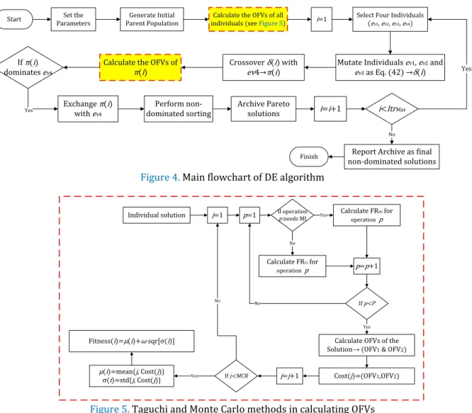
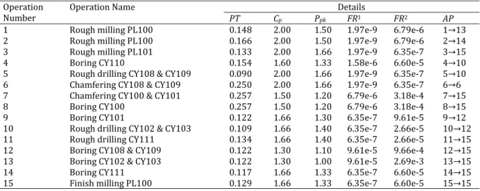
Figure 3 shows the flowchart of the DE algorithm and Figure 4 illustrates how Taguchi and Monte
Carlo methods are applied to take uncertainty of the parameters into account and calculated the robust objective functions.
Figure 4. Main flowchart of DE algorithm
Figure 5. Taguchi and Monte Carlo methods in calculating OFVs
6. Case study
6.1. Experiment design
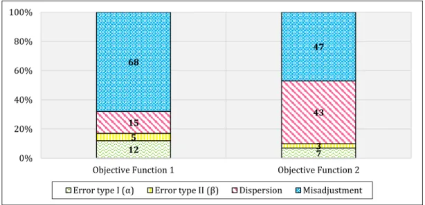
In order to validate the correctness of the proposed RBOMILP model and the evolutionary solution algorithm, a real industrial case is studied from one of the leading automotive industries in France. This case is a hydraulic pump with 15 quality characteristics. Figures 6 and 7, respectively, show the solid frame of the part and labeled quality characteristics which need to be inspected. Accordingly, some required deterministic information (i.e., without misadjustment) of the industrial case are tabulated as
Table 2, in which the first to sixth columns explain the name of operations, the production time, the
process capability Cp, the process performance Ppk and the failure rates with and without monitoring
inspection, respectively. Finally, the last column shows the allowable places (AP) that the inspections (i.e., CI and MI) can be performed at. For example, for the characteristic number 4 belonging to the operation “Boring CY110”, MI or CI can be performed only between operations 4 to 10. The DE algorithm is written in MATLAB 2014 and run using a computer with Intel Pentium 4, 2.3 GHz CPU and 4GB RAM.
Figure 6. Solid frame of the industrial part
Generate Initial Parent Population
Calculate the OFVs of all
individuals (see Figure 5)
Yes
i=1 Select Four Individuals
(ev1, ev2, ev3, ev4)
Mutate Individuals ev1, ev2 and
ev3 as Eq. (42) →δ(i)
i=i+1 i<ItrMax
Yes
Report Archive as final non-dominated solutions
No
Crossover δ(i) with
ev4→π(i) Calculate the OFVs of
π(i) If π(i) dominates ev4 Perform non-dominated sorting Set the Parameters Archive Pareto solutions Exchange π(i) with ev4 Start Finish
Individual solution j=1 p=1 If operation p needs MI
Calculate FRCI for operation p No Calculate FRMI for operation p Yes p=p+1 If p<P No
Calculate OFVs of the Solution→ (OFV1 & OFV2)
Yes Cost(j)=(OFV1,OFV2) j=j+1 If j<MCR No μ(i)=mean{j, Cost(j)} σ(i)=std{j, Cost(j)} Yes Fitness(i)=μ(i)+ω sqr[σ(i)]
Figure 7. Labeled operations of the industrial part
Table 2. Information of the industrial case
Operation
Number Operation Name PT Cp Ppk Details FR1 FR2 AP
1 Rough milling PL100 0.148 2.00 1.50 1.97e-9 6.79e-6 1→13 2 Rough milling PL100 0.166 2.00 1.50 1.97e-9 6.79e-6 2→14 3 Rough milling PL101 0.133 2.00 1.66 1.97e-9 6.35e-7 3→15 4 Boring CY110 0.154 1.60 1.33 1.58e-6 6.60e-5 4→10 5 Rough drilling CY108 & CY109 0.090 2.00 1.66 1.97e-9 6.35e-7 5→10 6 Chamfering CY108 & CY109 0.250 2.00 1.66 1.97e-9 6.35e-7 6→6 7 Chamfering CY100 & CY101 0.257 1.50 1.20 6.79e-6 3.18e-4 7→15 8 Boring CY100 0.257 1.50 1.20 6.79e-6 3.18e-4 8→15 9 Boring CY101 0.122 1.66 1.30 6.35e-7 9.61e-5 9→12 10 Rough drilling CY102 & CY103 0.109 1.66 1.40 6.35e-7 2.66e-5 10→12 11 Rough drilling CY111 0.134 1.66 1.40 6.35e-7 2.66e-5 11→15 12 Boring CY108 & CY109 0.122 1.30 1.10 9.61e-5 9.66e-4 12→15 13 Boring CY102 & CY103 0.122 1.30 1.00 9.61e-5 2.69e-3 13→15 14 Boring CY111 0.117 1.66 1.33 6.35e-7 6.60e-5 14→15 15 Finish milling PL100 0.129 1.66 1.33 6.35e-7 6.60e-5 15→15
6.2. Computational results
This section provides the results of the proposed global robust RBOMILP model. After applying the DE algorithm on the data of the hydraulic pump, the Pareto frontier of the RBOMILP model under the MI-and-CI strategy has been provided as Table 3 for both deterministic and uncertain models. In the deterministic model, all the parameters are deterministic and no uncertainty is imposed to the model. In the uncertain model, the parameters are manipulated in their corresponding alteration range as Table 1.
In Table 3, the first column shows the number of Pareto solutions. The second and the third columns
represent the values of the first and the second objective functions for the deterministic model. Similarly, the fourth and the fifth columns show the values of the first and the second objective functions for the uncertain model. Accordingly, twenty one and six Pareto solutions were obtained for deterministic and uncertain models, respectively.
Table 3. Pareto solutions of the RBOMILP model under MI-and-CI strategy
Pareto solution # Deterministic parameters Uncertain parameters
𝑂𝐹𝑉1 𝑂𝐹𝑉2 𝑂𝐹𝑉1 𝑂𝐹𝑉2 1 6077043 20900 6288260 44440 2 6076760 30800 5342750 322410 3 6076160 32340 5219250 1649230 4 6075560 55220 5130050 2328370 5 5970993 142670 5029200 5473050 6 5240900 165440 5014600 6467010 7 5240300 166980 - - 8 5185450 170060 - - 9 5164850 171600 - - 10 5154250 179300 - - 11 5143650 190740 - - 12 5143050 213620 - -
13 5138450 302500 - - 14 5097000 412830 - - 15 5066400 546150 - - 16 5055800 877470 - - 17 5054200 1357290 - - 18 5039600 2351250 - - 19 4964950 3630610 - - 20 4929750 5561930 - - 21 4910150 6555890 - -
Figure 8. Pareto frontiers for deterministic and uncertain models
The results of Table 3 have been illustrated in Figure 8, wherein dash and solid lines represent the Pareto frontier of the deterministic and the uncertain models, respectively. The inspection plans for different six Pareto solutions of the uncertain model have been depicted in Figure 9. As it can be seen, the solutions with the lower value of the first objective function, e.g., solutions number 5 and 6, represent the inspection plans with less number of MI and CI inspections. The reason is that the total internal cost (i.e.,
OFV1) is decreased by reducing the total cost of inspections (i.e., TCI), while the lower the inspection cost, the lower the number of inspection stations during the production process. On the other hand, solutions with the lower values of the warranty cost (i.e., OFV2) represent those inspection plans wherein the minimum nonconforming parts reach the customers. Accordingly, more numbers of inspections are performed in the inspection plans with lower values of OFV2. These different plans show the conflict of the total internal cost and the warranty costs and highlight the applicability and validity of the proposed RBOMILP.
Figure 9. Inspection plans of the Pareto solutions for the robust BMILP_EP
1 2 3 4 5 6 0 1 2 3 4 5 6 7 4,8 5 5,2 5,4 5,6 5,8 6 6,2 6,4 War ran ty Co st -OF V 2 ( 1 0 6)
Internal Cost - OFV2 (106)
Pareto Frontier_Uncertain Model Pareto Frontier_Deterministic Model
0
12 Q_CH: 7,8,10,11 15 Q_CH: 13-15 Q_CH: 8,11,13-15 6 Q_CH: 3,5,6 9 Q_CH: 1,4 Q_CH: 2,7,9,12 12 15 Q_CH: 7,8,11,12,15 Q_CH: 8,11-15 6 Q_CH: 6 10 Q_CH: 3,9,10 Q_CH: 2 11 Q_CH: 9,10 15 Q_CH: 7,8,11,12 6 Q_CH: 2,4,6 Q_CH: 11-15 11 Q_CH: 11,12 15 Q_CH: 7,13-15 10 Q_CH: 5,8-10 15 Q_CH: 7,8,11,12 12 Q_CH: 9-11 15 Q_CH: 12,13 11 Q_CH: 1,7,8 Pareto Sol #1 Pareto Sol #2 Pareto Sol #3 Pareto Sol #4 Pareto Sol #5 Pareto Sol #6Since in the real industrial case, the cost of CI is the same for all the quality characteristics, a quality characteristic undergoes the CI if that characteristic corresponds to an operation with low value of process capability CP. Accordingly, the operations with the lowest CP undergo CI one by one once the trade-off between two objective functions is met and the global minimum solution is found. The order of the process capability for different operations is 𝐶𝑃12= 𝐶𝑃13< 𝐶𝑃7= 𝐶𝑃8< 𝐶𝑃4= 𝐶𝑃9= 𝐶𝑃10= 𝐶𝑃11=
𝐶𝑃14= 𝐶𝑃15< 𝐶𝑃1= 𝐶𝑃2= 𝐶𝑃3= 𝐶𝑃5= 𝐶𝑃6. Accordingly, the quality characteristics created by
operations number 7, 8, 12 and 13 are more likely to undergo CI in every inspection plan.
Figure 10. Effect of uncertain parameters on the objective functions
Through an experiment, the contribution of the uncertain parameter in the increase of the objective functions was investigated to extract the parameters that impose high sensitivity to the objective functions. The result of this experiment has been depicted as Figure 9. As it can be seen, misadjustment and dispersion have the highest contribution on the objective functions’ sensitivity. In addition, misadjustment has higher effect on OFV1 rather than OFV2 and vice versa for dispersion. Therefore, the company of producing the hydraulic pump should have better control on the misadjustment if lower level of the internal cost is desired. It has been recommended to this company to limit the alteration and the uncertainty of the misadjustment as much as possible. On the other hand, if increasing the customer satisfaction (i.e., minimum warranty cost) is desired, limiting the variation of the both misadjustment and dispersion is recommended. Adragna et al. (2010) and Thornton (2004) have also proved the significant impact of misadjustment and dispersion in calculating inertial tolerancing and process capability index.
6.3. Sensitivity analysis
Hereafter, the effect of different uncertainty of parameters in which-what and when decisions are separately investigated. In addition, since the failure rate is affected by both misadjustment and dispersion, the effect of uncertainty in both of these parameters is also examined on the inspection decisions. Finally, a global robust inspection plan is obtained by considering all the parameters under uncertainty. The results are tabulated in Table 4, in which the first to third columns show different sources of uncertainty, the inspection strategy, and the total cost of manufacturing (𝑶𝑭𝑽𝟏+ 𝑶𝑭𝑽𝟐),
respectively. The fourth to tenth columns explain the contribution percent of each component to the total cost of manufacturing. Finally, the last two columns present those quality characteristics that need monitoring and conformity inspection, respectively. It should be noted that the value inserted in the parenthesis corresponds the location where inspection should be performed. For example, for the case of uncertainty in misadjustment under MI-or-CI, quality characteristics 1 to 6 need MI after operation 6, quality characteristics 9 to 11 need MI after operation 11, and quality characteristics 7, 8, and 12 to 15 need CI after operation 15. The first row of each inspection strategy corresponds to the deterministic model, wherein the parameters are deterministic and no alteration is allowed.
Table 4. Detail of cost objective function for different sources of uncertainty
Source of y g te ra𝑂𝐹 (St al ot T 𝑉 1 + 𝑂 𝐹 𝑉 2)
Detail Costs (%) Decisions
𝑂𝐹𝑉1 (% of Total) 𝑂𝐹𝑉2 (%) MI CI 12 7 5 3 15 43 68 47 0% 20% 40% 60% 80% 100%
Objective Function 1 Objective Function 2 Error type I (α) Error type II (β) Dispersion Misadjustment