To cite this document:
Barbiero, Franck and Vincent, François and Deloues, Thierry and
Letestu, Franck Effects of rotor blade modulation on GNSS anti-jamming algorithms.
(2014) In: ION International Technical Meeting, 27 January 2014 - 29 January 2014 (San
Diego, United States).
O
pen
A
rchive
T
oulouse
A
rchive
O
uverte (
OATAO
)
OATAO is an open access repository that collects the work of Toulouse researchers and
makes it freely available over the web where possible.
This is an author-deposited version published in:
http://oatao.univ-toulouse.fr/
Eprints ID: 11040
Any correspondence concerning this service should be sent to the repository
administrator:
[email protected]
Effects of rotor blade modulation on GNSS
anti-jamming algorithms
Franck Barbiéro (1)(2)(3), Francois Vincent(2), Thierry Deloues(1), Franck Letestu(3) (1) Office National d’Etudes et de Recherches aérospatiale (ONERA)
(2) Institut Supérieur de l’Aéronautique et de l’Espace. ISAE (3) THALES Avionics
BIOGRAPHY
Franck Barbiéro is a PhD student in the field of GNSS applications and adaptive processing in ONERA, a French aerospace research center. He graduated in 2011 as a signal processing engineer from the Grenoble Institute of Technology, France. His current research interests include adaptive antennas, radioelectrical propagation, signal processing, hardware implementation architectures and GNSS receiver.
Francois Vincent received the Engineer degree in electronics from ENSEEIHT, Toulouse, France in 1995, the PhD. Degree in signal processing from Toulouse University in 1999 and the "habilitation à diriger des recherches" from INPT, Toulouse in 2009. From 1999 to 2001, he was a research engineer with Siemens, Toulouse. He joined ISAE, Toulouse, France in 2001 and is currently an Associate Professor. His research interests include radar and navigation signal processing.
Thierry Deloues is a research engineer in the Signal Processing field at ONERA. His main research domain is the Antenna Signal Processing: adaptive array, autofocusing methods, and high resolution methods. He had worked on many projects concerning wideband and narrowband CCM, airborne high resolution localization, autofocusing arrays. He was involved also in NATO groups related to smart antennas, vibrating antennas and compensation techniques. At the moment, he is involved in antenna arrays design in the context of emitter's localization.
Franck Letestu is graduated engineer from CENTRALE, Lille, France, since 1996 and received an M.S degree from ISAE (Toulouse, France) in 1998. After having been involved in the development of radiofrequency front-end for GPS and GLONASS receivers in Brime SUD, he joined THALES in 2001 and contributes to the design of GNSS receivers, mainly for the RF and signal processing point of view. He acts currently as design authority for the development of controlled radiated pattern antenna products.
ABSTRACT
In hostile environment, Global Navigation Satellite System (GNSS) could be disturbed by intentional jamming. Many adaptive algorithms have been developed to deal with these threats, among which use of antenna arrays is one of the most efficient. However, most of them have been designed under stationary hypothesis and their performances in harsher environments are questionable. For instance, when a GNSS receiver is placed near rotating bodies, the signal undergo complex and non-stationary effects called Rotor Blade Modulation (RBM). These variations can degrade significantly anti-jamming performance. This paper investigates the impact of the RBM on three conventional space-time adaptive processing (STAP). First, to simulate the RBM, the signal received by an antenna mounted on a helicopter is computed thanks to electromagnetic (EM) asymptotic methods. Then, to quantify precisely the loss in performance of each algorithm, we compare post correlation carrier to noise ratio (post - C/N0) and covariance matrix estimation with respect of the time. Finally, the simulation results are confirmed by experiments conducted on an EC-120 helicopter with an L-band Continuous Wave (CW) jammer.
INTRODUCTION
Interference and multipath mitigation is one of the major challenges to improve Global Navigation Satellite System (GNSS) performance. Frequency mitigation techniques have shown limited results against wideband (WB) interferences. To overcome this drawback, one has investigated spatial filtering in adding more than one sensor. The mitigation is then improved by adding more degrees of freedom and then discriminate more easily the undesired signal. In the majority of adaptive space (or space-time) filtering techniques used in Controlled Reception Pattern Antenna (CRPA), the covariance matrix estimation is needed. Obviously in highly non-stationary environments, the common assumption of wide sense stationary is no longer valid and covariance matrix estimation exhibits strong mismatches leading to poor anti-jamming performances. Moreover, in presence of multipath (for example local antenna reflections), this covariance matrix does not represent anymore the exact
Direction of Arrival (DoA) of the different wavefronts because of the strong correlation between the paths. In these cases, the majority of adaptive processing drastically degrades. It's clearly the case when an antenna is placed near rotating bodies where these two negative issues occur. The rotation of the scatterers creates periodic time-varying effects on the phase and the amplitude of the received signal. Consequently, usual anti-jamming processing fails to reject these non-stationary effects. This phenomenon is well known as Rotor Blade Modulation (RBM) in the literature.
In this paper, we focus on the case of a GNSS antenna array placed under the main rotor of a helicopter and we investigate the effects of the RBM on standard GNSS anti-jamming methods. The effects of RBM on GNSS receivers have been experimentally studied [1], for instance by O'Brien et al. [2] but these approaches only focus on GNSS receiver measurements i.e. with fixed radiated pattern antenna (FRPA). A study conducted by Gupta et al. [3] deals with the same topic than our paper but its disclosure is restricted. Consequently, the existing literature on this subject is clearly very poor.
The present paper proposes to extend their studies to controlled radiated pattern antennas (CRPA). Our work covers three main areas: 1) ElectroMagnetic (EM) simulations of the RBM received signal, 2) effects on several adaptive algorithms performance, and 3) comparison of the simulations with real data.
In the first part, to characterize the RBM radio electric phenomenon, EM simulations are performed with the ONERA software "FERMAT" [4]. ONERA, the « Office National d’Etudes et de Recherches Aérospatiales (ONERA) », is a French aerospace research center. This software is based on hybridization between ray-launching and asymptotic methods such as Physical Optics (PO) or Equivalent Current Method (ECM). The simulations are performed with a 3D model of the helicopter of interest and they predict faithfully the EM field received by the RHCP antenna. These methods are perfectly adapted for L-band EM computations on such a complex scenario. Thus, the signature of the RBM could be investigated in Time-Frequency, Time-Delay and Direction of Arrival/Doppler domains. On this basis, we know how to compute the effect of the RBM on a jammer on the one hand and a wideband GNSS signal on the other hand. Then, in a second part, using this simulation of the RBM effects as an input, standard anti-jamming algorithms could be applied and compared. Power inversion (PI), Minimum Power Distortionless Response (MPDR) or Minimum Mean Square Error (MMSE) beamforming are reminded and tested to mitigate interference in presence of RBM. The loss in rejection performance is established by using post carrier to noise ratio (post - C/N0) that is to say after correlation with the local code within the GNSS receiver. As a matter of fact, it has been demonstrated [5] [6] that for GNSS applications, the common output pre-correlation Signal plus Interference to Noise Ratio (pre -
SINR) is not a sufficient criterion of performances. A deeper analysis could be conducted by showing carrier phase and delay code biases but the paper only focus on the C/N0 evaluation. The results show that, whatever the algorithms, the performances of rejection are strongly deteriorated in presence of RBM. A covariance matrix analysis is also conducted to explain this brake-down with interference.
Finally, to confirm EM simulation results, real data experiments are presented in a last part. The experiment involves a three blade helicopter landed on an airport and radiated by an interference source. A 2x2 square array GNSS right hand circularly polarized (RHCP) antenna is placed close to the helicopter under the main rotor. The jammer is a RHCP L-band wave located above the helicopter in order to cross the blades path. The experiment has been conducted with a Continuous Wave (CW) source with and without blade rotation.
ROTOR BLADE MODULATION SIMULATION AND ANALYSIS
This section describes the simulation scene and how the signal received by the antenna is computed in presence of the rotating bodies.
Two computations are done: on the one hand, we only consider the signal in his narrowband approximation. This method is sufficient to create jammer effects but is too restrictive to well characterize the channel for GNSS signals. On the other hand, we present the complete propagation effects. By keeping the information of delay and Doppler, this method perfectly represents effect of multipath on the received GNSS signal. These two approaches allow us representing precisely the RBM phenomenon in different applications.
Simulation scene
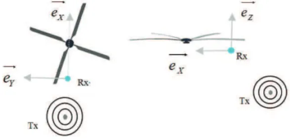
We consider 4 blades rotating at 393 rpm, with a length of 7.5m. The receiver is positioned 1m under the blade and 7m to the center of rotation. To simplify, we only focus on one position of the source in incidence and azimuth (151°, 180°). The figure 1 represents the simplest configuration of the scene with the blades only.
Figure 1- Simple configuration with rotating bodies only
Jammer computation
In this case, the received field will be compute thanks to the ONERA application FERMAT. This hybrid software is based on asymptotic methods, modeling interactions of an EM wave with a complex environment and predicting reliable electromagnetic fields in near and far field. The coupling of asymptotic methods and the Shooting and Bouncing Rays technique allows dealing with complex scenes, with high performances with a reduced computation time. These techniques are either ray-based (Geometrical Optics) or current-based (PO, ECM) which allow dealing with different diffraction problems (multi-bounds, surface, edge). The simulation is done in quasi-stationary state, that is to say a sample is compute for each “frozen” position of the blades. Then by adding the complex signal coming from every reflection with the Line of sight (LOS) signal, we obtain the complete received signal by an element of the array:
+
=
= N i t j i j LOS t f jA
e
LOSA
t
e
ie
t
y
1 ) ( . 2)
(
)
(
π0 φ φ(1)
N represents the number of reflections, f is the carrier 0
frequency. ALOS Ai φLOS, φi represent respectively the amplitude of the LOS signal and of the ith reflection, the phase of the LOS signal and of the ith reflection.
Figure 2- Normalised time power evolution and spectrum for 1 rotation of the blades for the L1 frequency with the source position in (151°,
180°).
Computation executed, we can first examine the influence of the presence of the LOS signal and the influence of the presence of the helicopter body on the received signal. Figure 2 represents the received power time variation during one rotor revolution and the corresponding Doppler spectrum for 3 configurations – LOS not present (Rotor reflected signals only-NLOS), rotor only reflections with LOS signal (LOS) and complete helicopter body reflected signals (NLOS+Helicopter). We can observe a minimum 20 dB mean power difference between NLOS and the LOS signal with a difference of less than 10 dB when the strongest reflection is present.
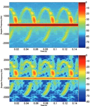
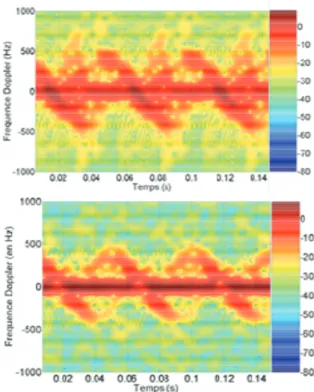
Figure 3- Normalised spectrogram of the rotor only with the LOS signal (top) and without LOS signal and with the body (bottom) with the source
position in (151°, 180°).
The amplitude modulation is less spiky when the helicopter body is considered because of the presence of a higher clutter floor level. Nevertheless the Doppler shape is not affected by the presence of the whole body. Hence, as we can see in figure 3, the time-frequency signature of the non-stationary channel is not significantly affected. Obviously, we can observe that the presence of the body increase the power of the static part of the scattering signals. This static body contribution is approximately 20 dB lower than the LOS power signal. It’s interesting to observe that for a jammer to signal ratio (J/S) of 70dB that is to say -90dBW, the multipath contribution is still more than 50 dB above the signal level.
To create the wideband jammer, we use the narrowband computation. Indeed, the impulse response computed for L1 carrier frequency could be supposed constant on the 40 MHz bandwidth. Consequently the received WB signal could be expressed as:
− =
+
=
/2 2 / 2 1 ) ()
(
)
(
B B ft j N i t j i j LOSe
A
t
e
e
df
A
t
y
φLOS φi π(2)
This formulation allows creating CW and WB jammer but GNSS signal can’t be computed thanks to the narrowband approximation.
GNSS signal computation
Since GNSS is Time-Of-Arrival (TOA) application, it’s necessary to keep the delay and Doppler information for each multipath to faithfully recreate the received signal. The use of Shooting and Bouncing Rays technique allows recovering the wideband information of each ray and characterizing different parameters of the overall received
signal such as:
- Angles of arrival
ϕ
kandθ
k - AmplitudeA
k- Phase
φ
k - Delay k - Dopplerν
kThe GNSS signal received by one sensor of the antenna, in wideband representation, is the sum of all the paths expressed as follow:
( )
[
(
(
)
)
]
= + + × − × − × = N k k k k k k ct d t j f t j A t y 1 0 2 exp ) ( ) ( τ τ π ν φ(3)
where c and d are respectively the modulation code and the navigation message. N is the number of paths.
Figure 4- Impulse response for 1 rotation of the 4 blades for the L1 frequency with the source position in (151°, 180°).
It can be observed on figure 4 the time variation of the normalised impulse response without LOS and without helicopter body. The time-varying channel is here determined with accuracy. For satellite incoming signal, it’s understandable that the knowledge of the time varying antenna pattern is not enough to describe the effect of the RBM on the signal of interest. On the contrary, with the time-varying impulse response, the channel is perfectly known and then the impact of the RBM on adaptive processing and covariance matrix estimation could be tackled.
COMMON ADAPTIVE ALGORITHMS
In this section, we recall some theoretical points about common STAP algorithms [5][7].
Consider an array of m sensors illuminated by one useful and one jamming signals (respectively
u
andj
), the antenna output in static case can be written as:( )
n
=
a
uu
( )
n
+
a
jj
(
n
)
+
η
(
n
)
y
(4)
where
η
(n
)
is a White Gaussian Noise.a
uanda
jdenote the steering vectors of the array. Single sensor radiation patterns are included into the steering vectors. In presence of RBM, the output can be written as:
( )
n
=
f
RBM(
a
uu
( )
n
+
a
jj
(
n
)
)
+
η
(
n
)
y
(5)
The adaptive architecture consists in weighting the receiving samples. The complex beamformer weight vector w is controlled in phase and amplitude by the array processor to give the nullformer output:
( )
n
( )
n
y
out=
w
Hy
(6)
With
- m the number of antenna.
-
y
( )
n
the antenna output signal of size [m, Nsnap].-
w
=
[
w
1w
m]
m×1 the weighting vector. -y
out( )
n
the output filtering signal.The superscript .H stands for Hermitian transform. For each position of sensor, we simulate the RBM channel response for GNSS signal and jammer as input. For the rest of the paper, for convenience, we use the notation of “n” to describe the sample at the time “nTs”
where Ts is the sample period.
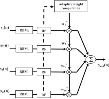
Figure 5- Architecture scheme of the simulator of the RBM impact on SAP algorithm.
The weight is designed to reject the undesired interference or also to preserve the GNSS signal. Numerous
w1* RBM1 yout(n) RF
Σ
w2* RBM1 RF w3* RBM1 RF wm* RBM1 RF Adaptive weight computation s1(n) s2(n) s3(n) sm(n)algorithms have been developed depending on the applications and the specifications of the embedded system.
We chose to consider three algorithms: - “Power inversion”
- “Minimum Power Distortionless Response” - “Minimum Mean Square Error”
Power Inversion
The first one is called Power Inversion. It’s the simplest to implement since it doesn’t need any knowledge about the DOA of the signal of interest.
The weight vector is:
c
R
c
c
R
w
1 1 − −=
H PI(7)
where:-
R
is the sample covariance matrix estimation. -c
=
[
0
...
0
1
0
...
0
]
mOnly one reference tap is non-zero. This blind method is not optimal but particularly useful when no information about the possible direction of arrival of the desired signal is available. The nulling is done in the directions of the most powerful incident signals but no preservation is guaranteed in any other direction.
Minimum Power Directional Response
This second algorithm is known to maximize the SNR as minimizing the total output power while preserving a unitary gain in the signal of interest direction.
The weight vector is:
)
,
(
)
,
(
)
,
(
0 0 1 0 0 0 0 1ϕ
θ
ϕ
θ
ϕ
θ
a
R
a
a
R
w
− −=
H MVDR(8)
Where:-
a
(
θ
0,
ϕ
0)
is the directional vector of the desired signal.Minimum Mean Square Error
The Minimum Mean Square Error consists in minimizing the difference between the STAP output signal and a desired reference signal. The reference
x
refis the local Pseudo Random Noise (PRN) code of the considered satellite.The weight vector is:
ref MMSE
R
r
w
=
−1(9)
We define the cross correlation between the beamformer output and the local code as:
( )
( )
[
*]
n
x
n
E
ref refy
r
=
(10)
It also relaxes calibration constraints existing in MPDR. We can observe that every algorithms presented in this section are based on the covariance matrix. In practice, this matrix is unknown and has to be estimated. The most common way to conduct this estimation is time sample averaging:
( ) ( )
==
SNAP N n SNAPn
n
N
1 *1
ˆ
y
y
R
(11)
with NSNAP the number of samples used to the estimation.
But this estimation is no longer valid in case of strong non-stationary environments and performances of associated algorithms drastically degrade as presented in the following part.
CORRELATION MATRIX DURING ROTOR BLADE MODULATION
This section analyzes the impact of the RBM on the covariance matrix of the array.
Algorithms not relying on this matrix estimation (Eq. 9) use iterative methods to solve weight vector with convergent time highly dependent on jamming conditions (sensitivity to eigenvalue spread). They are no further described in this paper because their performances under non-stationary conditions are obviously worse than snapshot methods described here.
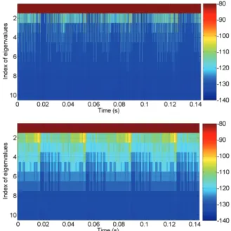
It will be assumed that the received signal is a L1 GPS C/A code with 20MHz bandwidth. The received power of the desired signal is -150dBW. The angles of incidence of the signal of interest are 60° for elevation and 30° for azimuth. The antenna is 2x2 wavelength size squared array. We add a CW jammer of -90dBW with angles of incidence of 151° for elevation and 180° for azimut. No Doppler frequency shift is added for the GNSS incident signal or the jammer. The number of the predominant eigenvalues of the covariance matrix gives a good indication on the size of the jammer subspace to be rejected. In figure 6, the time variation of the power of the eigenvalues is presented for two estimation duration: 100us and 1ms. Only the interference subspace comes out of the noise floor. The GNSS signal keeps under this floor and cannot be seen on the eigenvalues before the correlation step. In stationary case, the CW jammer consumes only one degree of freedom i.e. the associated LOS eigenvector has a dimension 1. However, in presence of RBM, it can be observed a spreading of
associated eigenvalues. These intermediate values, between LOS and noise, actually represent other interferences due to scattering on rotating bodies. The figure 6 shows that the scattering interference is a short-term phenomenon and increasing the estimation time of the covariance matrix smoothes the time variation of the eigenvalues. Nevertheless, it could also degrade the estimation because of non-stationarities.
To conclude this section, we observe a fast time-varying spread of the number of eigenvalues corresponding to the reflections on the rotating parts. It's now necessary to study if the estimation of these eigenvectors is enough accurate to mitigate the jammer.
Figure 6- Time variation of the power of eigenvalues of the covariance matrix with an estimation time of 100us and 1ms. IMPACT OF THE RBM: SIMULATIONS
In this second part, jammer mitigation provided by the three adaptive algorithms is evaluated in different configurations.
Static case without blades
To begin, the rejection is evaluated in a static case without blades, only with a LOS CW signal.
Figure 7- Time variation of pre-correlation SINR.
Figure 8- Time variation of post C/N0.
The channel is stationary. SINR and C/N0 are obviously quite constants and the rejection and acquisition are efficient.
Dynamic case with RBM
Then, analysis of SINR and C/N0 with respect to time is considered in presence of RBM (fig. 9 to 14). The configuration is the same than in the previous parts i.e. with the four blades and the three algorithms are evaluated. Four cases are considered for the time-average estimation of covariance matrix: 10us, 100us, 1ms and 10ms. The time of integration for the acquisition step is 1ms for the first third cases and 10ms for the fourth.
Discussions
Conventional adaptive algorithms reject correctly the RBM reflections only if the estimation time of the covariance matrix is short enough. The three algorithms allow a correct acquisition process for an estimation time of the covariance matrix below 1ms. If this condition is not fulfilled, the stationary part of the signal is rejected but the fast time varying part is not well estimated and the rejection is not complete. Consequently the signal is not well protected and the phase of acquisition could be deteriorated by the non-rejected residual interferences.
The consequence of this condition is a high computation load (covariance matrix estimation and inversion) which is very difficult to tackle for real-time applications.
Iterative Vs Snapshot implementation
The computation of the adaptive weight could be completed in two main different ways: iterative or "snapshot" implementations. The snapshot version consists in computing the weight vector on a fixed estimation time and in applying to the same samples the adaptive solution. The extreme simplicity of the recursive version is clearly an attractive feature. Nevertheless, its convergence relies on the eigenvalues spread of the covariance matrix, and in practical situations it is often too slow. Consequently, iterative algorithms are no further described in this paper since their performances under non-stationary conditions are obviously worse than snapshot methods [9].
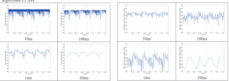
Algorithm PI SAP
10us 100us
1ms 10ms
Figure 9- Time variation of SINR versus estimation time of the covariance matrix with PI SAP
Algorithm MMSE
10us 100us
1ms 10ms
Figure 11- Time variation of SINR versus estimation time of the covariance matrix with MMSE
Algorithm MPDR STAP
10us 100us
1ms 10ms
Figure 13- Time variation of SINR versus estimation time of the covariance matrix with MPDR STAP
10us 100us
1ms 10ms
Figure 10- Time variation of C/N0 versus estimation time of the covariance matrix with PI SAP
10us 100us
1ms 10ms
Figure 12- Time variation of C/N0 versus estimation time of the covariance matrix with MMSE
10us 100us
1ms 10ms
Figure 14- Time variation of C/N0 versus estimation time of the covariance matrix with MPDR STAP
IMPACT OF THE RBM: EXPERIMENTATIONS
This last section presents the experimentations conducted with a real helicopter. A comparison with simulation is conducted.
Experimental Scene
This experiment involves a three blade EC-120 helicopter landed on an airport. A 2x2 array GNSS right hand circularly polarized (RHCP) antenna is placed at the right hand side, under the main rotor as illustrated in figure 15. The source is a monochromatic RHCP L-band wave located on the tower close to the helicopter in order to cross the blades path. This configuration is not optimal to study the backscattered waves from the blades but an underneath source configuration would be difficult to reproduce. Moreover, this landed configuration also increases the impact of all the static bodies of the scene and the possible multi-rebound path. At last all the dielectric characteristics of the objects in the environment are difficult to estimate. Consequently, all objects are defined as Perfectly Electrical Conductor (PEC).
Figure 15- Experimental scene with the EC-120 helicopter (jammer view)
Figure 16- Experimental scene with the EC-120 helicopter (lateral view)
For safety reasons, the experiments have not been conducted with the antenna mounted on the helicopter that’s why the antenna is placed on the left of the helicopter.
To compare exactly simulation and experiments we chose to recreate the scene and compare the Time-Frequency variations. Figure 17 shows the model of the scene with the FERMAT tools.
Figure 17- Reproduction of the experimental scene with the EC-120 helicopter
EM simulations perfectly match the experiments. The RBM effects are well simulated and the time-frequency analysis of the signal shows the similar frequency modulation in both cases. But even if the same dynamic appear, some fading effects are created because of the definition of materials of the floor and the building (fig. 18).
Figure 18- Normalised spectrogram of the 3 blades for the L1 frequency with the FERMAT simulation (top) and real data (bottom). By using the received signal as input of the conventional adaptive algorithms, a degradation of the rejection is observed if the estimation time of the
GNSS
receiver
Jammer
GNSS
receiver
Jammer
GNSS
receiver
Jammer
covariance matrix is too high. These observations are the same that in the simulation process.
CONCLUSION
In this paper, we have analyzed the impact of the RBM on adaptive antenna using conventional space-time adaptive processing. First, an electromagnetic simulation has been performed and very good match with measurements has been shown. Then, the performances of sample based covariance matrix algorithms have been evaluated in non-stationary environments. Time variation of eigenvalues, signal to interference plus noise ratio and carrier-to-noise ratio have been shown for various covariance estimation time. A significant degradation of most commonly used adaptive SAP or STAP algorithms have been shown for estimation time superior to few milliseconds. However, the shorter the estimation time of the covariance matrix, the better the performances. The consequence is a high computation load (covariance matrix estimation and inversion) which is very difficult to tackle for real-time applications and, obviously, performance of iterative algorithms are worse under such non-stationary conditions.
REFERENCES
[1] Stevens, J.R.A., Brodin, G.J., Cooper, J.A.,
"Measuring the Effect of Helicopter Rotors on GPS Reception," Proceedings of the 2004 National Technical Meeting of The Institute of Navigation, San Diego, CA, January 2004, pp. 962-973.
[2] O'Brien, A.J., Hayhurst, K., Gupta, I.J., "Effects of
Rotor Blade Modulation on GNSS Receiver
Measurements," Proceedings of the 22nd International Technical Meeting of The Satellite Division of the Institute of Navigation (ION GNSS 2009), Savannah, GA, September 2009, pp. 2352-2361.
[3] A. Svendsen and I.J. Gupta, “Effects of Rotor
Modulation on the Nulling Performance of GNSS Adaptive Antennas” Proceedings of Joint Navigation Conference, Orlando, FL, June 2009.
[4] H. Mametsa, S. Laybros, A. Berges, P. Combes, P. N’Guyen, and P. Pitot. “FERMAT: A high frequency em
scattering code from complex scenes including objects and environment”. In: Antennas and Propagation, 2006. EuCAP 2006. First European Conference on, pp. 1–4, 2006.
[5] G. Carrie, “Technique d’antennes adaptatives pour
récepteurs de radionavigation par satellites résistant aux interférences” PhD thesis, Ecole Nationale Supérieure de l’Aéronautique et de l’Espace, Décembre 2006.
[6] O'Brien, A.J.; Gupta, I.J., “Comparison of Output
SINR and Receiver C/N0 for GNSS Adaptive Antennas,”
IEEE Transactions on Aerospace and Electronic Systems, Volume 45, Issue 4, October 2009, pp. 1630-1640. [7] Van Trees H.L “Optimum Array Processing, Part IV
od detection, Estimation and Modulation Theory”
WILEY-INTERSCIENCE 2002.
[8] Kaplan E.D. “Understanding GPS: Principles and
Applications” 1996 Artech House inc.
[9] F. Letestu, D. Depraz “Dimensioning parameters for
Anti-jamming and Controlled Radiation Pattern Antenna Systems” Proceedings of the Korean GNSS Society Conference (KGS 2013), Jeju, Korea, November 2013.