LIDAR WAVEFORM MODELING USING A MARKED POINT PROCESS

HAL Id: hal-00781804

https://hal.inria.fr/hal-00781804

Submitted on 28 Jan 2013

HAL is a multi-disciplinary open access

archive for the deposit and dissemination of

sci-entific research documents, whether they are

pub-lished or not. The documents may come from

teaching and research institutions in France or

abroad, or from public or private research centers.

L’archive ouverte pluridisciplinaire HAL, est

destinée au dépôt et à la diffusion de documents

scientifiques de niveau recherche, publiés ou non,

émanant des établissements d’enseignement et de

recherche français ou étrangers, des laboratoires

publics ou privés.

LIDAR WAVEFORM MODELING USING A

MARKED POINT PROCESS

Clément Mallet, Florent Lafarge, Frédéric Bretar, Uwe Soergel, Christian

Heipke

To cite this version:

Clément Mallet, Florent Lafarge, Frédéric Bretar, Uwe Soergel, Christian Heipke. LIDAR

WAVE-FORM MODELING USING A MARKED POINT PROCESS. International Conference on Image

Processing (ICIP), Nov 2009, Cairo, Egypt. �hal-00781804�

LIDAR WAVEFORM MODELING USING A MARKED POINT PROCESS

Cl´ement Mallet

, Florent Lafarge

, Fr´ed´eric Bretar

, Uwe Soergel

, Christian Heipke

1

Laboratoire MATIS, Institut G´eographique National - Saint-Mand´e, FRANCE –

2

IMAGINE, Universit´e Paris Est, France - Marne-la-Vall´ee, FRANCE –

3

IPI, Leibniz Universit¨at Hannover - Hannover, GERMANY –

ABSTRACT

Lidar waveforms are 1D signal consisting of a train of echoes where each of them correspond to a scattering target of the Earth sur-face. Modeling these echoes with the appropriate parametric func-tion is necessary to retrieve physical informafunc-tion about these objects and characterize their properties. This paper presents a marked point process based model to reconstruct a lidar signal in terms of a set of parametric functions. The model takes into account both a data term which measures the coherence between the models and the wave-forms, and a regularizing term which introduces physical knowledge on the reconstructed signal. We search for the best configuration of functions by performing a Reversible Jump Markov Chain Monte Carlo sampler coupled with a simulated annealing. Results are fi-nally presented on different kinds of signals in urban areas.

Index Terms— Signal reconstruction, Lidar, Source modeling, Marked point process, RJMCMC, 3D point cloud.

1. INTRODUCTION

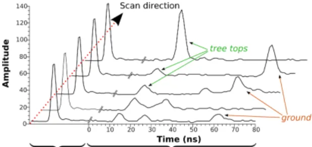
Airborne laser scanning is an active remote sensing technique pro-viding range data as georeferenced 3D point clouds. It enables fast, reliable, accurate, but irregular mapping of both terrain and elevated features such as the tree canopy and the ground underneath. The new technology of full-waveform lidar systems permits to record the backscattered signal for each transmitted laser pulse (i.e., an intensity histogram). Instead of clouds of individual 3D points, lidar devices provide connected 1D profiles of the 3D scene, which contain more detailed information about the structure of the illumi-nated surfaces [1]. Indeed, each signal consists of series of temporal modes (called echoes), where each of them corresponds to an indi-vidual reflection from an object (see Figure 1).

Thus, the decomposition of the waveforms allows first to find the

Fig. 1. Example of consecutive lidar waveforms.

3D location of the targets. Besides, modeling each echo with a suitable analytical function permits to retrieve its shape, which can provide relevant features for segmentation/classification algorithms

[2]. Lidar signal reconstruction is then a topic of major interest. The conventional methods for reconstructing 1D signals such as wavelets, splines [3] or Gaussian mixture models [4] are not partic-ularly adapted since they are too general, do not always model each mode of the waveform and do not take into account the physical characteristics of lidar waveforms. Some specific lidar algorithms have been proposed using for instance the non-linear least-square approach [5]. However, the gradient computation required in such models limits both the introduction of physical knowledge on the waveforms and the type of the chosen function.

Stochastic approaches based on marked point processes [6] are very promising for addressing the issue of reconstructing lidar wave-forms. These models have shown good potentialities for many applications in image analysis such as the extraction of road net-work [7], vascular trees [8] or 3D urban objects [9]. Our method simulates mixtures of various parametric functions representing the reconstructed echos. An energy is associated to each configuration and the global minimum is then found using a Reversible Jump Markov Chain Monte Carlo (RJMCMC) algorithm [10]. Our model presents several interesting characteristics compared to conventional waveform modeling techniques mentionned above:

• Multiple function types - It allows to deal with various types of parametric functions. By using a library of shapes, more accurate estimates are performed compared to classical approaches such as the Gaussian mixture one [11].

• Lidar physical knowledge integration - Complex prior infor-mation on lidar waveform characteristics can be introduced in the energy without having problems of convexity or/and continuity re-strictions in the formulation of these interactions.

• Efficient exploration of configuration spaces - A RJMCMC sampler with relevant proposition kernels allows to avoid exhautive explorations of continuous configuration spaces, and is particularly efficient when the number of functions is unknown. Generally speaking, the MCMC samplers offer good potentialities in signal reconstruction [12], and for instance in lidar waveform estimate for counting and locating the reflected returns from surfaces [13]. The proposed model is formulated in Section 2. Section 3 describes the optimization procedure. Results are then shown in Section 4 as well as 3D point clouds generated from our approach. Finally, conclusions and perspectives are drawn.

2. MODEL DEFINITION 2.1. Marked point processes

A marked point process in S= K × M is a point process living in a continuous bounded set K supporting a1D-signal where each point is associated with a mark specifying an object [6]. In our method, each lidar waveform is modeled by a marked point process with K=

[0, Nmax] , where Nmaxis the size of the waveform and M , the mark

space. The objects of the process are parametric functions taken from a predefined library. They are described by a certain number of random variables corresponding to their parameters. The marked point process is specified by a density function f(.) w.r.t a measure of reference (i.e., the Poisson measure). This density, which allows to take into account complex interactions between objects, is usually expressed using a Gibbs energy U(.) (i.e., f ∝ exp −U ). In order to find the configuration x of functions that better fits the waveforms, we estimate the global minimum of U by coupling a MCMC sampler with a simulated annealing.

2.2. Library of modelling functions

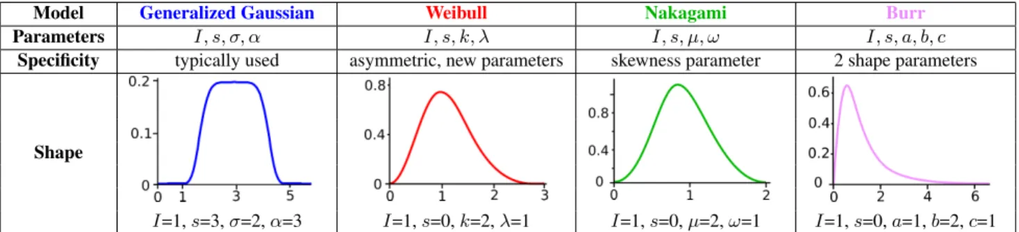
The contents of the library is a key point since the function param-eters will be used afterwards for classifying 3D point clouds. The Generalized Gaussian (GG) model has been shown to fit most of the echoes of lidar waveforms in urban areas [2]. Nevertheless, this as-sumption is not always sufficient and new functions are introduced both to fit asymmetric echoes (echoes are slightly distorted by roof materials and ground surface) and symmetric ones but with other pa-rameters than those provided by the GG model. For instance, the GG model gives the amplitude and width for symmetric echoes whereas the Weibull distribution provides a scale and a shape parameter and the Burr one simulates asymmetric modes (cf. Table 1).

2.3. Energy formulation

Let x be a configuration of parametric functions (or objects) xi

ex-tracted from the above library. The energy U(x) measuring the qual-ity of x is composed of both a data term Ud(x) and a regularization

one Up(x) such as:

U(x) = β Ud(x) + (1 − β) Up(x) (1)

where β ∈ [0, 1] tunes the trade-off between the prior energy and the data term.

2.3.1. Data energy

The data energy helps the model to best fit to the lidar waveforms. The likelihood can then be obtained by computing a distance be-tween the given signalSdataand the estimated one ˆS, which depends

on the current objects on the configuration x. Ud(x) = s 1 |K| Z K ( ˆS − Sdata)2 (2)

This term, which measures the quadratic error between both signals, allows to be sensitive to high variations i.e., to local strong errors in signal estimate.

2.3.2. Prior energy

Up(x) allows to introduce interactions between objects of x, and to

favor/penalize some configurations. For aerial lidar waveforms, the prior knowledge is set up by physical limitations in the backscatter of lidar pulses.

Up(x) = Un(x) + Ue(x) +

X

xi∼xj

Um(xi, xj) (3)

where xi∼ xjconstitutes the set of neighboring objects in the

con-figuration x. This neighborhood relationship∼ is defined as follow:

xi∼ xj= {(xi, xj) ∈ x | |µxi− µxj| ≤ r} (4)

µxi (resp. µxj) represents the mode (i.e., the position of the

maxi-mum amplitude of the echo) of the associated function to object xi

(resp. xj), and r is the lidar sensor range resolution (i.e., the

mini-mum distance between two objects along the laser line of sight that can be differentiated).

(i) Echo number limitation The two first echoes of a waveform con-tain in general about 90% of the total reflected signal power. Con-sequently, even for complex targets like forested areas, a waveform empirically reaches a maximum of seven echoes and it is quite rare to find more than four echoes. In urban areas, most of the targets are rigid, opaque structures like buildings and streets. Thus, more than two echoes are usually found in non dense trees. We then aim to favor configurations with a limited number of objets with an energy given by:

Un(x) = − log Pcard(x) with ∞

X

n=0

Pn= 1 (5)

where Pnis the probability for the waveform to have n echoes. The

probabilities are empirically set up by a coarse mode estimate on a urban test area. Here, we have: P1 = 0.6, P2 = 0.27, P3 = 0.1

and P46n67= 0.01. For n > 7, Un(x) is set to a positive hardcore

value.

(ii) Backscattered energy limitation As an airborne laser system cannot physically receive a signal with an higher energy than emit-ted, it is possible to formulate a backscattered energy based on this property.

Ue(x) = ωe1{E(x)>Eref}(E(x) − Eref)

2

(6) where 1{.}is the characteristic function, E(x) =

R

KSxis the

en-ergy of the configuration x, compared to a reference power Eref, set

with the knowledge of the emitted lidar power. Only waveforms with superior energy are penalized: no assumption can be formulated on the received energy since it depends on the target properties. (iii) Sensor range resolution limitation We aim to penalize objects spatially closer along the line of sight than the sensor range resolu-tion. Such energy is given by:

Um(xi, xj) = ωmexp r2− |µxi− µxj| 2 σ2 ! (7) and also permits to favor configurations with a small number of ob-jects. Indeed, a single pulse can be fitted by an important number of echoes but such situation does not reflect the reality.

2.3.3. Parameter settings

Physical and weight parameters can be distinguished. Physical pa-rameters are r and σ. We choose σ= 0.01 ns and r = 5 ns. Data and regularizing terms are weighted one compared to the other, re-spectively with a factor β set to 0.5. The two prior weights are tuned by “trial-and-error” tests.

3. OPTIMIZATION

We aim to find the configuration of objects which minimizes the non convex energy U in a variable dimension space since the number of objects is unknown and function types are defined by different num-ber of parameters. Such a space can be efficiently explored using a Reversible Jump Markov Chain Monte Carlo (RJMCMC) sampler

Model Generalized Gaussian Weibull Nakagami Burr

Parameters I, s, σ, α I, s, k, λ I, s, µ, ω I, s, a, b, c Specificity typically used asymmetric, new parameters skewness parameter 2 shape parameters

Shape

I=1, s=3, σ=2, α=3 I=1, s=0, k=2, λ=1 I=1, s=0, µ=2, ω=1 I=1, s=0, a=1, b=2, c=1 Table 1. Library of models. I and s are common parameters to all functions, respectively for amplitude and shift or location.

coupled with a simulated annealing.

The RJMCMC sampler [10] consists in simulating a discrete Markov Chain (Xt), t∈ N on the configuration space, having an invariant

measure specified by the energy U . This sampler performs ”jumps” between spaces of different dimensions respecting the reversibility assumption of the chain. One of the advantage of this iterative algo-rithm is that it does not depend on the initial state. The jumps are realized according to three kinds of move called proposition kernels: • Perturbation kernel: the parameters of an object belonging to the current configuration x is modified;

• Birth-and-death kernel: an object is added or removed from the current configuration x and

• Switching kernel: the type of an object belonging to x is switched with another type of the library.

The probabilities of choosing each move are equal since no assump-tion can be made on which move is more relevant at the current state. A simulated annealing is used to ensure the convergence pro-cess. A relaxation parameter Tt, defined by a sequence of

tempera-tures decreasing to zero when t→ ∞, is introduced in the RJMCMC sampler (i.e., U(.) is substitued by U(.)_T

t ). The simulated annealing

allows to theoretically ensure the convergence to the global optimum for all initial configuration x0 using a logarithmic temperature

de-crease. In practice, we prefer using a geometrical cooling scheme which is faster and gives an approximate solution close to the opti-mal one. During the temperature decrease, the process explores the configurations of interest and becomes more and more selective. It corresponds to local adjustments of the object of the configuration. To sum up the optimization process, if at t, Xt= x

1. Choose randomly one of the proposition kernel Qi;

2. According to Qi, choose a new configuration y from x;

3. Take Xt+1= y with a probability

min » 1, Qi(y → x) Qi(x → y) exp −„ U (y) − U (x) Tt «–

and take Xt+1= x otherwise.

4. RESULTS 4.1. Experiments on simulated signals

To assess the reliability of the algorithm, it has been first applied on signals with a higher complexity than real lidar waveforms. Longer signals with more echoes than physically expected, with distorted and overlapping modes as well as corrupted with noise have been

fitted with our method. One just has to tune the prior physical pa-rameters to extend the energetical formulation to other kinds of sig-nals. To deal respectively with very close echoes and with large overlapping ones, the interaction between objects can be changed by decreasing and increasing r and σ. To reconstruct signals with higher energy, Erefcan be tuned. To fit signals with more modes, the

echo number limitation can be modified by accepting more echoes within the signal and with the same probability.

Figure 2 shows that good fitting results can be achieved on simulated waveforms, even corrupted with Gaussian noise, by tuning prior pa-rameters, assessing the reliability of the algorithm on 1D random signals. The nine echo locations are accurately found. However, small differences between the reference and the estimated signals can be locally noticed, especially with noisy signals where the algo-rithm has more difficulties to find the exact maxima and fit the upper parts of the modes (e.g., 2ndand 4thechoes in Figure 2b).

Fig. 2. Results of complex waveform fitting on a simulated signal with nine echoes (left) and on the same signal with Gaussian noise (right). The dotted black line and the continuous grey one are re-spectively the raw and the reconstructed signals.

4.2. Airborne lidar waveforms

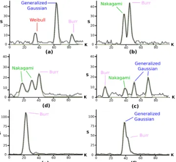
Waveforms acquired from an airborne lidar system over different kinds of landscapes have been analysed using the marked point pro-cess approach. Figure 4 shows results both on urban (buildings) and natural (trees, hedges) items. The right number of echoes is found as well as the correct shape of the waveform: single and multiple overlapping echoes are retrieved, even in vegetated areas where the noise level is significant w.r.t. the echo amplitudes (Figures 4c and d).

The Generalized Gaussian, Weibull and Nakagami functions have been introduced to model the same kind of echoes. Thus, there is no concluding whether the minimal configurations obtained are com-posed of the right modeling functions. As expected, the Burr model allows to fit slightly asymmetric echoes, especially the second echo of two overlapping ones (Figures 4b, d and f).

Fig. 3. Results of waveform decomposition on a urban area with dense trees and complex buildings. Left: orthoimage of the test area c IGN. Middle: resulting 3D point cloud (Blue: low elevation→ brown: high elevation) over the whole area. Right: results over two trees showing that points inside tree canopy are retrieved.

Fig. 4. Example of decomposed and modeled waveforms on (a-d) trees, (e) a building roof and (f) a hedge.

area to assess the reliability of the method in a complex and hetero-geneous landscape. A waveform-by-waveform evaluation of the fit-ting process to estimate the correctness of the echo detection would be highly time-consuming. Thus, the algorithm has been rather eval-uated by computing the relative amplitude error ε on each signal with the L∞norm to detect missing echoes. For that purpose, the

noise within raw signals is first removed. Finally, the mean error computed on 80000 signals is ε=4.1%: the ground and buildings waveforms are fitted with lower amplitude error (εa=3.4%) than

veg-etation ones (εv=7.9%). The weak difference between εaand εvcan

be explained by the fact that waveforms over vegetated areas have much more complex shapes than over anthropic surfaces but have much lower amplitudes (see Figure 4).

The waveform decomposition allows to retrieve the mode of each echo which corresponds to the range between the sensor and a target. The 3D cartographic coordinates of each echo can then be computed from the range values using georeferencing formulas. Figure 3 dis-plays the resulting 3D point cloud of this process over the test area, which can be now classified using the estimated parameters of mod-eling functions as performed in [2].

5. CONCLUSION AND FUTURE WORKS

We have proposed an original method for modeling airborne lidar waveform by complex parametric functions. The obtained results are satisfactory. The proposed marked point process approach is well adapted both to locate echoes in signals and accurately describe them with parametric functions. 3D points can therefore be gen-erated over large areas with echo shape descriptors taken from the

extensible model library and offer the possibility to improve classi-cal lidar point cloud classification algorithm. Moreover the physiclassi-cal parameters of the proposed energy are tunable and offer the possibil-ity to extend the method to other kinds of signals and lidar sensors (terrestrial and spatial).

Finally, in future works, it would be interesting to estimate automat-ically the weighting parameters using for instance the Expectation-Maximizationalgorithm. Moreover, we should introduce in the en-ergy formulation specific interactions between parametric functions of different types in order to improve local signal adjustments.

6. REFERENCES

[1] C. Mallet and F. Bretar, “Full-waveform topographic lidar: State-of-the-art,” ISPRS Journal of Photogrammetry and Re-mote Sensing, vol. 64, no. 1, pp. 1–16, 2009.

[2] C. Mallet, F. Bretar, and U. Soergel, “Analysis of Full-Waveform Lidar Data for Classification of Urban Areas,” Pho-togrammetrie Fernerkundung Geoinformation, vol. 5, pp. 337– 349, 2008.

[3] M. Unser, “Splines: A Perfect Fit for Signal and Image Pro-cessing,” IEEE Signal Processing Magazine, vol. 16, no. 6, pp. 22–38, 1999.

[4] A. El-Baz and G. Gimel’farb, “EM Based Approximation of Empirical Distributions with Linear Combinations of Discrete Gaussians,” in IEEE ICIP, 2007.

[5] M.A. Hofton, J.B. Minster, and J.B. Blair, “Decomposition of Laser Altimeter Waveforms,” IEEE Trans. on Geoscience and Remote Sensing, vol. 38, no. 4, pp. 1989–1996, 2000. [6] M.N. Van Lieshout, Markov point processes and their

appli-cations, Imperial College Press, London, 2000.

[7] C. Lacoste, X. Descombes, and J. Zerubia, “Point processes for unsupervised line network extraction in remote sensing,” IEEE Trans. on Pattern Analysis and Machine Intelligence, vol. 27, no. 2, pp. 1568–1579, 2005.

[8] K. Sun, N. Sang, and T. Zhang, “Marked Point Process for Vas-cular Tree Extraction on Angiogram,” in EMMCVPR, 2007. [9] F. Lafarge, X. Descombes, J. Zerubia, and M.

Pierrot-Deseilligny, “Building reconstruction from a single DEM,” in IEEE CVPR, 2008.

[10] P.J. Green, “Reversible Jump Markov Chain Monte-Carlo computation and Bayesian model determination,” Biometrika, vol. 82, no. 4, pp. 97–109, 1995.

[11] D. Salas-Gonz´alez, E. Kuruoglu, and D. Ruiz, “Bayesian es-timation of mixtures of skewed alpha stable distributions with an unknown number of components,” in EUSIPCO, 2006. [12] E. Punskaya, C. Andrieu, A. Doucet, and W. Fitzgerald,

“Bayesian curve fitting using MCMC with applications to sig-nal segmentation,” IEEE Trans. on Sigsig-nal Processing, vol. 50, no. 3, pp. 747–758, 2002.

[13] S. Hern´andez-Mar´ın, A. Wallace, and G. Gibson, “Bayesian Analysis of Lidar Signals with Multiple Returns,” IEEE Trans. on Pattern Analysis and Machine Intelligence, vol. 29, no. 12, pp. 2170–2180, 2007.