2008-02
RIBONI, Alessandro
RUGE-MURCIA, Francisco J.
Monetary Policy by Committee:Consensus,
Chairman Dominance or Simple Majority?
Département de sciences économiques Université de Montréal
Faculté des arts et des sciences C.P. 6128, succursale Centre-Ville Montréal (Québec) H3C 3J7 Canada http://www.sceco.umontreal.ca [email protected] Téléphone : (514) 343-6539 Télécopieur : (514) 343-7221
Ce cahier a également été publié par le Centre interuniversitaire de recherche en économie quantitative (CIREQ) sous le numéro 02-2008.
This working paper was also published by the Center for Interuniversity Research in Quantitative Economics (CIREQ), under number 02-2008.
Monetary Policy by Committee:
Consensus, Chairman Dominance
or Simple Majority?
Alessandro Riboni
yand Francisco J. Ruge-Murcia
zJanuary 2008
Abstract
This paper studies the theoretical and empirical implications of monetary policy making by committee under three di erent voting protocols. The protocols are a consensus model, where super-majority is required for a policy change; an agenda-setting model, where the chairman controls the agenda; and a simple majority model, where policy is determined by the median member. These protocols give preeminence to di erent aspects of the actual decision making process and capture the observed heterogeneity in formal procedures across central banks. The models are estimated by Maximum Likelihood using interest rate decisions by the committees of ve central banks, namely the Bank of Canada, the Bank of England, the European Central Bank, the Swedish Riksbank, and the U.S. Federal Reserve. For all central banks, results indicate that the consensus model is statistically superior to the alternative models. This suggests that despite institutional di erences, committees share unwritten rules and informal procedures that deliver observationally equivalent policy decisions. JEL Classi cation: D7, E5
Key Words: Committees, voting models, status-quo bias, median voter.
We received helpful comments from Pohan Fong and participants in the Research Workshop on Monetary Policy Committees held at the Bank of Norway in September 2007. This research received the nancial support of the Social Sciences and Humanities Research Council of Canada. Correspondence: Alessandro Riboni, Departement de sciences economiques, Universite de Montreal, C.P. 6128, succursale Centre-ville, Montreal (Quebec) H3C 3J7, Canada.
yDepartement de sciences economiques, Universite de Montreal
\I try to forge a consensus : : : . If a discussion were to lead to a narrow majority, then it is more likely that I would postpone a decision." (Wim Duisenberg, former President of the ECB, The New York Times, 27 June 2001)
1
Introduction
An important question in economics concerns the implications of collective decision making on policy outcomes. Prominent examples of decisions taken by a group of heterogeneous individuals, rather than by a single agent, include scal and monetary policy. Decisions concerning public spending, taxation and debt are taken by legislatures,1 while the target
for the key nominal interest rate is selected by a committee in most central banks.
This paper develops a model where members of a monetary policy committee have dif-ferent views regarding the optimal interest rate and resolve those di erences through voting. First, the equilibrium outcome is solved under various voting (or bargaining) protocols. Then, their respective theoretical and empirical implications are derived, and all models are estimated by the method of Maximum Likelihood using data on interest rate decisions by the committees in ve central banks. The central banks are the Bank of Canada, the Bank of England, the European Central Bank, the Swedish Riksbank and the U.S. Federal Reserve. Finally, model selection criteria are used to compare the predictive power of the competing theories of collective choice.2
Since there is institutional evidence of heterogeneity in the formal procedures employed by monetary committees to arrive at a decision (see, for example, Fry et al., 2000), we study three voting protocols. Each protocol gives preeminence to di erent aspects of the actual decision making process. The rst protocol is a consensus-based model where a super-majority (that is, a level of support which exceeds a simple super-majority) is required to adopt a new policy and no committee member has proposal power. The second protocol is the agenda-setting model, originally proposed by Romer and Rosenthal (1978), where decisions are taken by simple majority and the chairman is assumed to control the agenda. These two protocols yield outcomes di erent from the median policy and predict an inaction region (or gridlock interval) where the committee keeps the interest rate unchanged. In addition, they deliver endogenous autocorrelation and regime switches in the interest rate. However,
1Among the theoretical contributions that examine the consequences of legislative bargaining are Baron
(1991), Chari and Cole (1993), Persson et al. (2000), Battaglini and Coate (2007a, 2007b), and Volden and Wiseman (2007).
2Previous literature on monetary committees usually relies on the Median Voter Theorem and focuses on
features other than the voting procedure. For instance, Waller (1992, 2000) study the implications of the length of the term of o ce and of the committee size, respectively.
these protocols generate di erent implications for the size of interest rate adjustments: the agenda-setting model predicts larger interest rate increases (decreases) than the consensus model when the chairman is more hawkish (dovish) than the median member. The third protocol is a simple-majority model where no member controls the agenda, all alternatives are put to a vote and, consequently, the interest rate selected by the committee is the one preferred by the median member. This protocol is observationally equivalent to a setup where the median is the single central banker.
According to survey results reported in Fry et al. (2000), a little more than half of the monetary policy committees in their sample (43 out of 79) make decisions by consensus, while the rest hold a formal vote. Of the ve central banks studied in this paper, only one (the Bank of Canada) explicitly operates on a consensus basis while the remaining ones hold a formal vote by simple majority rule. However, the distinction is ambiguous in practice because consensus appears to play a role in the decision making process of committees that (on paper) take decisions by simple majority rule.3 Committees also seem to di er with
respect to the role played by the chairman. In some committees, the chairman can exert leadership, in particular by deciding the content of the proposal that is put to a vote.4 For example, a prevalent view is that under the mandate of Alan Greenspan, agreement within the Federal Open Market Committee (FOMC) was dictated by the chairman.5 A consequence of the agenda-setting power of the chairman is that the nal voting outcome may sometimes be di erent from the policy favored by a majority of members.6 On the
other hand, strong leadership does not necessarily mean that the chairman is de facto a single decision maker.7 This discussion suggests that institutional and anecdotal evidence
alone cannot unambiguously reveal how monetary policy committees reach decisions. As an alternative strategy to understand central banking by committee, we pursue instead
3See, for example, the interview of Wim Duisenberg with the The New York Times cited at the beginning
of this paper.
4This is case, for instance, in the monetary committees of the Bank of England, the Norges Bank, Reserve
Bank of Australia, the Swedish Riksbank, and the U.S. Federal Reserve (see Meier, 2007).
5Blinder (2004, p. 47) remarks that \each member other than Alan Greenspan has had only one real choice
when the roll was called: whether to go on record as supporting or opposing the chairman's recommendation, which will prevail in any case."
6Blinder (2004, p. 47) cites two instances where this appears to have been true for the FOMC. First,
transcripts for the meeting on 4 February 1994 indicate that most members wanted to raise the Federal Funds rate by 50 basis points, while Greenspan wanted a 25 point increase. Nonetheless, the committee eventually passed Greenspan's preferred policy. Second, Blinder reports the general opinion that in the late 1990s Greenspan was able to maintain the status quo although most committee members were in favor of an interest rate increase.
7For example, former FOMC members Sherman Maisel (1973, p. 124) and Laurence Meyer (2004, p. 52)
respectively observe that the Chairman \does not make policy alone" and \does not necessarily always get his way."
the direct econometric analysis of actual policy outcomes and the use of stochastic simulation to derive quantitative predictions which are then compared with the data. Our econometric results show that despite the heterogeneity in the formal procedures followed by the monetary committees in our sample, the consensus-based model describes interest rate decisions more accurately than the alternative models for all ve central banks studied. Overall these results suggest that, in addition to the formal framework under which committees operate, their decision making is also the result of unwritten rules and informal procedures that deliver observationally equivalent policy decisions.
The data also show limited empirical success on the part of the median model. One of the reasons is that this model predicts lower interest rate autocorrelation than it is found in the data. Instead, by introducing a status-quo bias, the consensus-based model is better able to capture this feature of the data. This means, in particular, that consensus can provide a politico-economic explanation for the well known observation in that central banks adjust interest rates more cautiously than predicted by standard models.
Finally, regarding the agenda-setting model, the data indicate that even if the chairman has proposal power, his policy recommendation will take into account the preferences of the other committee members. Furthermore, there is very limited empirical support for agenda control on the part of the chairman as modeled by Romer and Rosenthal (1978). This con rms, using actual data, earlier ndings based on laboratory experiments (see, for example, Eavey and Miller, 1984).
These results should be of interest to monetary economists concerned with understanding the implications of committees on central banking, as well as to political economists and political scientists interested in testing the implications of competing theories of committee bargaining. Indeed, monetary policy committees provide an ideal setup to study group policy making because voting outcomes and status quo locations are well-de ned in the data and decisions concern only one dimension (i.e., the interest rate), thereby reducing the possibility of logrolling.8
The remainder of the paper is organized as follows. Section 2 describes the committee and its decision making under the three di erent voting procedures. Section 3 estimates the models and compares their empirical results. Section 4 concludes.
8A few empirical contributions in the area of legislative studies compare di erent theories of committee
decision making. For example, Krehbiel et al. (2005) test the predictive power of the pivot and cartel theories of law making in the U.S. Senate using frequencies of cutpoint estimates, that is, estimates of the roll-call-speci c location that splits the \yea" side from the \nay" side. However, that literature faces the problems that bargaining is potentially multi-dimensional, that bill and status quo locations are di cult to observe and measure, and that ideal points are not estimated on the same scale as bill locations. To overcome these obstacles, many researchers have turned to laboratory experiments to test theories of committee bargaining. See Palfrey (2005) for a review of the experimental literature.
2
Committee Decision Making
2.1
Composition and Preferences
Consider a monetary policy committee composed of N members, labelled j = 1; ::::; N; where N is an odd integer.9 The committee is concerned with selecting the value of the policy
instrument in every meeting. The policy instrument is assumed to be the nominal interest rate, it. The alternatives that can be considered by the committee belong to the continuos
and bounded set I = 0; i : The relation between the policy instrument and economic outcomes is spelled out below in Section 2.2.
The utility function of member j is E 1 X t= tU j( t) ! ; (1)
where 2 (0; 1) is the discount factor, tis the rate of in ation, and Uj( ) is the instantaneous
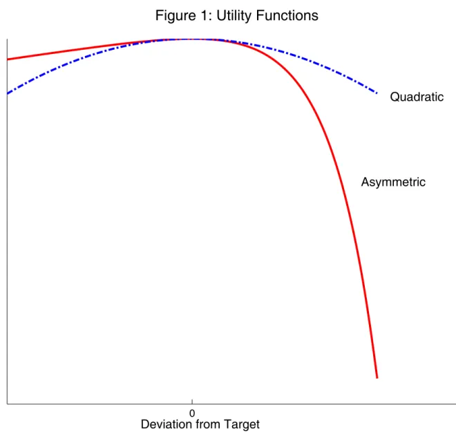
utility function. The instantaneous utility function is represented by the asymmetric linex function (Varian, 1974), Uj( t) = exp ( j( t )) + j( t ) + 1 2 j ; (2)
where is an in ation target and j is a member-speci c preference parameter. This
functional form generalizes the standard quadratic function used in earlier literature and permits di erent weights for positive and negative in ation deviations from the target.10
For example, when j > 0; a positive deviation from causes a larger decrease in utility
than a negative deviation of the same magnitude. The reason is that for in ation rates above ; the exponential term dominates and utility decreases exponentially, while for in ation rates below ; the linear term dominates and utility decreases linearly. Intuitively, when
j > 0, committee member j is more averse to positive than to negative in ation deviations
from the target even if their size (in absolute value) is identical. In order to develop the readers' intuition, the quadratic and asymmetric utility functions are plotted in Figure 1.
For this asymmetric utility function, the coe cient of relative prudence (Kimball, 1990) is j( t ); which is directly proportional to the in ation deviation from its desired value
with coe cient of proportionality j: The assumption that committee members di er in
9The assumption that N is odd allow us to uniquely pin down the median committee member and
eliminates the complications associated with tie votes. Erhart and Vasquez-Paz (2007) nd that in a sample of 79 monetary policy committees, 57 have an odd number of members with 5, 7 and 9 the most common observations.
10To see that the function (2) nest the quadratic case, take the limit of U
j( t) as j ! 0 and use L'Hopital's
their relative prudence is a tractable way to motivate disagreement over preferred interest rates despite the fact that members share the same in ation target.11 We order the N
committee members so that member 1 (N ) is the one with the smallest (largest) value of : That is, 1 6 2 6 ::: 6 N: The median member, denoted by M , is the one with
index (N + 1)=2 and, for simplicity, his preference parameter is normalized to be zero, that is, M = 0.12 We will see below in Section 2.3 that heterogeneity in preference parameters
implies that indirect utilities, expressed as a function of the policy instrument it, attain
di erent maxima depending on j.
2.2
Economic Environment
As in Svensson (1997), the behavior of the private sector is described in terms of a Phillips curve and an aggregate demand curve:
t+1 = t+ 1yt+ "t+1;
yt+1 = 1yt 2(it t) + t+1;
where yt is the deviation of an output measure from its natural level, 1; 2 > 0 and 0 < 1 < 1 are constant parameters, and "t and t are disturbances. The persistence of the
disturbances is modeled by means of moving average (MA) processes "t = ut 1+ ut;
t = &vt 1+ vt;
where ; & 2 ( 1; 1); so that the processes are invertible, and ut and vt are mutually
inde-pendent innovations. The innovations are Normally distributed white noises with zero mean and constant conditional variances 2u and v2; respectively. This speci cation embodies a stylized mechanism for the transmission of monetary policy and is widely used in the lit-erature on monetary policy committees (see, among others, Bhattacharjee and Holly, 2006, Gerlach-Kristen, 2007, and Weber, 2007). After some algebra, one can write
t+2 = (1 + 1 2) t+ 1(1 + 1)yt 1 2it+ "t+1+ 1 t+1+ "t+2: (3)
As a result of the control lag in this model, the interest rate selected by the committee at time t a ects in ation only after two periods via its e ect on the output gap after one period.
11We use this modeling strategy because, except for the U.S., all countries in our sample follow in ation
targeting regimes. However, our results hold more generally and are robust, for example, to assuming instead quadratic utility and heterogeneous in ation targets.
12For the empirical part of this project, we will also require that the cross-sectional distribution of is
time-invariant, meaning that even when there are changes in the composition of the committee (for example, as a result of alternation of voting members), the preference parameters remain unchanged.
2.3
Policy Preferred by Individual Members
Since monetary policy takes two periods to have an e ect on in ation, consider the member-speci c interest rate ij;t chosen at time t to maximize the expected utility of member j at time t + 2. That is,
ij;t = arg max
fitg
2E
tUj( t+2);
subject to equation (3). Equation (3) combines the Phillips and aggregate demand curves and summarizes the constraints imposed by the private sector on the policy choices of the committee. The rst-order necessary condition of this problem is
2( 1 2) Et jexp ( j( t+2 )) j 2 j = 0: which implies Etexp ( j( t+2 )) = 1: (4)
Under the assumption that innovations are Normally distributed and conditionally ho-moskedastic, the rate of in ation at time t + 2 (conditional on the information set at time t) is Normally distributed and conditionally homoskedastic as well. Then, exp ( j( t+2 ))
is distributed Log-normal with mean exp j(Et t+2 ) + 2j 2=2 where 2 is the
condi-tional variance of t: Then, substituting in (4) and taking logs,
Et t+2 = j 2=2: (5)
Finally, taking conditional expectations as of time t in both sides of (3) and using (5) deliver member j's preferred interest rate
ij;t = aj + b t+ cyt+ t; (6) where aj = 1 1 2 + j 2 1 2 2 ; b = 1 + 1 1 2 ; c = 1 + 1 2 t = 1 2 ut+ & 2 vt:
This reaction function implies that if the current output gap or in ation increase, the nominal interest rate should be raised in order to keep the in ation forecast close to the in ation target. Note, however, that ex-post in ation will typically di er from because of the disturbances that occur during the control lag period. As a result of this uncertainty, the asymmetry in the utility function will induce a prudence motive in the conduct of monetary policy and ij;twill also depend on in ation volatility in proportion to j. Hence, the intercept
term in the reaction function is member-speci c (and hence the subscript j in aj). Notice, for
example that committee members who weight more heavily positive than negative in ation deviations from its target (i.e., those with j > 0) will generally favor higher interest rates.
On the other hand, the coe cients of in ation (b) and the output gap (c), and the disturbance tdepend only on aggregate parameters (and aggregate shocks in the latter case)
and, consequently, they are common to all members. Since individual reaction functions di er in their intercepts only, it is easy to see that ordering members according to ; that is,
1 6 2 6 ::: 6 N; translates into an ordering of preferred interest rates, i1;t 6 i2;t 6 : : : 6
iN;t:
Finally, since the innovations ut and vt are white noise, then t is also white noise and
its constant conditional variance is 2 = 2 u2=( 1 2)2+ &2 v2=( 2)2:
2.4
Protocol I: Consensus
In order to model the idea of consensus, this protocol assumes that proposals to adopt a new interest rate require a super-majority to pass. Super-majority is a majority greater than 50 percent plus one of the votes, or simple majority. Under this protocol, no committee member controls the agenda: the set of alternatives that are put to a vote is chosen according to a predetermined rule. Let qt denote the status quo policy in the current meeting and
assume that the initial status quo is the interest rate, it 1; that was selected in the previous
meeting. The state of the economy, which is known and predetermined at the beginning of the meeting, is given by st ( t; yt; t) : There are two stages in each meeting. In the
rst stage, members vote by simple majority rule whether the debate in the second stage will involve an increase or a decrease of the interest rate with respect to the status quo. If the committee votes for an interest rate increase (decrease), all alternatives that are strictly smaller (larger) than qt are immediately discarded.
In the second stage, the committee selects the interest rate among the remaining alter-natives through a binary agenda with a super-majority required for a proposal to pass.13 A
binary agenda is a procedure where the nal outcome chosen by the committee is the result
of a sequence of pairwise votes (see Austen-Smith and Banks, 2005, Ch. 4, for a discussion). Let S (N +1+2K)=2 denote the size of the smallest super-majority required for a proposal to pass. The size of the super-majority increases in the index K, where 06 K 6 (N 1)=2: This speci cation includes as special cases unanimity, when K = (N 1)=2; and simple majority, when K = 0: Since the case where K = 0 delivers the median outcome and is equivalent to the protocol studied in Section 2.6, in what follows, we concentrate on cases where 16 K 6 (N 1)=2.
The voting procedure is as follows. Suppose, for example, that in the rst stage the committee decided to consider an increase of the interest rate. Then, the alternative qt+
is put to a vote against the status quo qt; where > 0. If qt+ does not meet the approval
of a super-majority of members, then the proposal does not pass, the meeting ends and the status quo is implemented. If the proposal passes, then qt+ displaces qt (= it 1) as the
default policy and the meeting continues with the alternative qt+ 2 voted against qt+ .
If qt+ 2 does not pass, the nal decision becomes qt+ : If the proposal passes, then qt+ 2
displaces qt + as default policy, the alternative qt + 3 is voted against qt + 2 ; and so
on. For the sake of the exposition and to avoid unnecessary complications, assume that all alternatives and all member-speci c preferred interest rates (from equation (6)) are integer multiples of .
Note that the number of possible rounds in the second stage of each meeting is nite. Let r denote the round, with r = 1; :::; R: If the committee keeps accepting further increases, there will be a nal round R where the committee will have to chose between i and i :14
We study pure strategy subgame perfect equilibria with the property that, in each period, individuals vote as if they are pivotal. This re nement is standard in the voting literature and rules out equilibria where a committee member votes contrary to his preferences simply because changing his vote would not alter the voting outcome. Furthermore, throughout this paper, it is assumed that committee members are forward looking within each meeting (that is, they vote strategically in each round of the meeting foreseeing the e ect of their vote on future rounds), but they abstract from the consequences of their voting decision on future meetings via the status quo.
Let (st; qt; !t) denote the political aggregator under a consensus-based voting protocol,
where !t is the vector of induced policy preferences over the interest rate for all committee
members. For all states st and qt, the stationary function ( ) aggregates the induced
policy preferences into a policy outcome. The next proposition shows that the protocol described above delivers a simple equilibrium outcome. For status quo policies that are
14Alternatively, if in the rst stage of the meeting the committee decides to consider interest rate decreases
located close to the median's preferred policy, the committee does not change the interest rate. For status quo policy that are su ciently extreme, compared with the values preferred by most members, the committee adopts a new policy that is closer to the median outcome. Proposition 1: The policy outcome in the consensus model is given by
it = (st; qt; !t) = 8 < : iM +K;t; if qt> iM +K;t; qt; if iM K;t6 qt6 iM +K;t; iM K;t; if qt< iM K;t:
Proof: Note that for each committee member, the induced preferences over the interest rate are strictly concave and, consequently, single peaked with peak given by (6). The proof consists of the following steps.
Step 1: De ne the undominated set U (st; !t) of the super-majority relation in set I as the
set of alternatives that are not defeated in a direct vote against any alternative in I. The setU (st; !t) contains all alternatives in the interval iM K;t; iM +K;t .
Step 2: We claim that if any policy in U (st; !t) is the default in any round r, that policy
must be the nal outcome of the meeting at time t. This is obviously true in the nal round R. We prove that this is true in any round by induction. Suppose that is true at round r + 1; we show that this is true at round r as well. Suppose that at round r an interest rate i belonging to U (st; !t) is the default and, nevertheless, another policy i0 passes and
moves to round r + 1. There are two cases: either i0 also belongs to the undominated set or it does not. In the former case, we know that i0 will be the nal decision according to our inductive hypothesis. But this would mean that a super-majority prefers i0 to i. This
contradict the fact that i belongs to the undominated set. Suppose instead that i0 does
not belong to the undominated set. Notice that this implies that the alternatives that will be considered in future rounds, including R, will not belong to U (st; !t). This is the case
because the undominated set is an interval. Then the nal outcome must not belong to U (st; !t) : This contradicts the hypothesis that i belongs to the undominated set.
Step 3: By Step 2, we know that if qt2 U (st; !t), qtwill be the nal outcome. This explains
why it= qt if iM K;t6 qt6 iM +K;t: If instead qt2 U (s= t; !t), we know that there is only one
direction (either an increase or a decrease from the status quo) that allows the committee to eventually reach an alternative in U (st; !t). It is easy to see that the committee chooses
that direction in the rst stage. By doing so, in a nite number of rounds, the committee will vote between either iM +K;t and iM +K;t + or between iM K;t and iM K;t : At that round, the alternative in the undominated set will pass and will be the nal outcome. This explains why if qt < iM K;t (or respectively, qt> iM +K;t); the committee decides to consider
an increase (respectively, a decrease) of the interest rate that will eventually lead to iM K;t (respectively, iM +K;t) as the nal outcome. {
Intuitively, for an initial status quo qt > iM +K;t; members initially agree on decreasing
the nominal rate and successive proposals are passed until it= iM +K;t: When it= iM +K;t, a
further -decrease would not receive the approval of a super-majority of members and the nal decision will be it= iM +K;t: Similarly, for an initial status quo qt< iM K;t; members initially
agree on increasing the nominal rate and successive proposals are passed until it = iM K;t:
When it = iM K;t, a further -increase would not receive the approval of a super-majority
of members and the nal decision will be it = iM K;t: Finally, for an initial status quo
iM K;t 6 qt6 iM +K;tand regardless of the result in the rst stage of the meeting, no proposal
would pass in the second stage and the interest rate will remain unchanged, it = it 1.
Notice that this protocol features a gridlock interval, that is, a set of status quo policies where policy changes are not possible. The gridlock interval includes all status quo policies qt 2 [iM K;t; iM +K;t] and its width is increasing in the size of the super-majority, K. The
super-majority requirement induces a status-quo bias because it demands the agreement of most members for a policy change. The policy outcome as a function of qt under this
protocol is plotted in Panel A of Figure 2. Policies on the 45 degree line correspond to it = qt; meaning that the interest rate remains unchanged after the committee meeting.
Since the median outcome occurs only in the special case where the status quo coincides with the policy preferred by the median (that, qt = iM;t); it follows that consensus implies
deviations from the median outcome.
2.5
Protocol II: Agenda-Setting by a Dominant Chairman
In this model, proposals are passed by simple majority rule but members di er in their institutional role. In particular, the chairman sets the agenda and makes a policy proposal to the other committee members in every meeting. This represents the idea that chairmen have more power and in uence than their peers stemming, for instance, from prestige or additional responsibilities.
In what follows, the chairman is denoted by A and the median by M: It is also assumed that A 6= M:15 Thus, there are two possible cases: either A > M or A < M: In
the case where A > M ( A < M); the chairman is hawkish (dovish) in the sense that,
conditional on in ation, in ation volatility and the output gap, he systematically prefers a
15The case
A= M is trivial in that it always delivers the median outcome, and it is therefore
higher (lower) interest rate than M . For the sake of exposition, this Section focuses on the case of the hawkish chairman only, but the dovish case is perfectly symmetric.
The voting protocol is the following. In each meeting, given the current status quo qt = it 1, the chairman proposes an interest rate it under close rule. The other committee
members can either accept or reject the chairman's proposal. If the proposal passes (i.e., it obtains at least (N + 1)=2 votes), then the proposed policy is implemented and becomes the status quo for next meeting. If the proposal is rejected, then the status quo is maintained and it = it 1. This procedure is repeated in the next meeting. As in the consensus
model, individuals vote as if they were pivotal and disregard the consequences of their voting decision on future meetings via the status quo. Thus, members accept a proposal whenever the current utility from the proposal is larger than or equal to the utility from the current status quo, and the chairman picks the policy closest to his ideal point among those that are acceptable to a majority of (N + 1)=2 members. This voting game is well-known in the political economy literature and was originally derived by Romer and Rosenthal (1978) under the assumption of symmetric preferences. Here instead, the induced utilities of all members other than the median are single peaked but not symmetric. In principle, this lack of symmetry may imply that proposals are accepted by a coalition that excludes the median. The proof of Proposition 2 insures that this is not the case.
De ne (st; qt; !t) to be the political aggregator in the agenda-setting game. The
following proposition establishes the policy outcome under this protocol.
Proposition 2: The policy outcome in the agenda-setting model with A> M is given by
it = (st; qt; !t) = 8 > > < > > : iA;t; if qt > iA;t; qt; if iM;t6 qt6 iA;t; 2iM;t qt; if 2iM;t iA;t6 qt< iM;t; iA;t; if qt < 2iM;t iA;t; :
Proof: The proof consists of the following steps.
Step 1: Let Vj(:) denote the indirect utility of member j as a function of the interest rate
and let it denote the current proposal. We show that Vj(it) Vj(qt) is increasing in j for
all it and qt such that qt 6 iM;t 6 it. The di erence of the expected payo of committee
member j associated to interest rates it and qt is
Vj(it) Vj(qt) =
exp (%t) (exp( j 1 2qt) exp( j 1 2it)) + j 1 2(qt it) 2
j
where %t= (1 + 1 2) t+ 1(1 + 1)yt+ j2 2=2 + ut+ & 1vt: When qt6 iM;t6 it, it can
in j is that 2j 2 > 2 for all j > M. In the rest of the proof we will assume that this
condition is veri ed.
Step 2: First, when qt 2 (iA; i]; the agenda setter proposes iA;t; which is accepted by all
members j such that J 6 A: This follows from the indirect utility being single-peaked.
When qt2 [iM;t; iA;t], the agenda setter cannot increase the interest rate. The best proposal
among the acceptable ones is the status quo, which is always accepted. When qt 2 [2iM;t
iA;t; iM;t), the set of policies that the median accepts is given by the interval [qt; 2iM;t qt]:
By Step 1, we know that these proposals are accepted by all members j such that J > M
and that any proposal greater than 2iM;t qt; which is rejected by the median, is also rejected
by all members j such that J 6 M: Finally, when qt2 [0; 2iM;t iA;t); the agenda setter
is again able to propose iA; which is accepted by the median. By Step 1 this proposal is also accepted by all members j such that J > M: {
The political aggregator as a function of qt is plotted in Panel B of Figure 2. The
policy aggregator for the case of a dovish chairman is plotted in Panel C of the same gure, and it is easy to see that it is the mirror image of the one derived here for the hawkish chairman. The control over the agenda of the part of the chairman implies deviations from the median outcome. This is due to the fact that the chairman can propose the policy he prefers, among those alternatives that at least a majority of committee members (weakly) prefer to the status quo. Among the acceptable alternatives, there is no reason to expect the chairman to propose the median outcome. Moreover, deviations from the median outcome are systematically in one direction. That is, they will always bring the policy outcome closer to the policy preferred by the chairman.
As before there is an interval of status quo policies for which policy change is not possible (i.e., a gridlock interval). This interval is given by [iM;t; iA;t], that is all policies between the interest rate preferred by the median and the chairman. If the status quo falls within this interval, policy changes are blocked by either the chairman or a majority of committee members. To see this, note that when qt 2 [iM;t; iA;t], a majority would veto any increase
of the instrument value towards iA and proposing the status quo is then the best option for the chairman. The width of the gridlock interval is increasing in the distance between the chairman's and the median's preferred interest rates.
A policy change occurs only if the status quo is su ciently extreme, compared with the members' preferred policies. In particular, when qt falls in the interval [2iM;t iA;t; iM;t),
the chairman chooses the policy closest to his ideal point subject to the constraint that M will accept it. This constraint is binding in equilibrium meaning that M will be indi erent between the status quo and the interest rate that A proposes. Since the median has a
symmetric induced utility (recall that M = 0), this proposal is the re ection point of qt
with respect to iM;t: When the status quo policy is either lower than 2iM;t iA;t or higher than iA;t; the chairman is able to o er and pass the proposal that coincides with his ideal point.
In the rest of this Section, we compare the theoretical predictions of the consensus and agenda-setting models. First, both models deliver a gridlock interval where it is not possible to change the status quo. However, it is di cult to predict a priori which voting procedure features the largest gridlock interval because the comparison depends on the degree of con-sensus that the committee requires (summarized by K) and on the extent of disagreement between the chairman and the median. The intersection of the two intervals is non-empty given that iM;t must belong to both gridlock intervals. In principle, the gridlock interval in the agenda-setting model could be a strict subset of the one in the consensus model if j A Mj is su ciently small and K su ciently large, but the converse cannot happen.
Second, whenever the committee decides to change the status quo, the models deliver di erent predictions with respect to the size of the policy change. The agenda-setting model with hawkish (dovish) chairman yields more aggressive interest rate increases (decreases) than the other two models. For example, suppose that the chairman is a hawk. Then, when qt < iM;t, the agenda-setting model unambiguously predicts a larger policy change
compared with the consensus model. Instead, when qt> iM;t; the comparison is ambiguous
and the size of the interest rate decrease depends on the location of iA;t versus iM +K;t: Finally, note that under both protocols, the endpoints of the gridlock interval are sto-chastic and depend on current state of the economy. An implication of the predicted local inertia is that the relation between changes in the state of nature and in policy is nonlinear. In particular, small changes in the state of economy are less likely to produce policy changes compared with larger ones. Empirically, this would mean, for example, that small variations in the rates of in ation and unemployment are less likely to result in a change in the key nominal interest rate, compared with large movements in these variables.
2.6
Protocol III: Simple-Majority Model
The Median Voter Theorem (Black, 1958) dictates that when preferences are single-peaked, N is odd, and the policy space is one-dimensional, there is a unique core outcome, represented by the alternative preferred by the individual whose ideal point constitutes the median of the set of ideal points. In our set-up, which satis es all the conditions of the theorem, this alternative is represented by
where iM;t is the interest rate preferred by the median member. In its original formulation, the Median Voter Theorem lacks a non-cooperative underpinning. However, one can show that when its conditions are satis ed, the nal outcome of any binary agenda under simple majority (irrespective of the order through which alternatives are put to a vote) will imple-ment the median's ideal point. For instance, policy iM;t will be the nal outcome of the binary agenda in Section 2.4 as long as one requires simple majority, that is S = (N + 1)=2: It is interesting to note that under simple majority, inertia and path dependence disap-pear. Within each meeting, starting from any status quo policy, the interest rate preferred by the median individual is always selected. Having a committee is then equivalent to having the median committee member as a single central banker and the reaction function is observationally indistinguishable from a standard Taylor rule derived under the assump-tion that monetary policy is selected by one individual. The model predicts a proporassump-tional adjustment of the policy instrument in response to any change in in ation and unemploy-ment regardless of their size and generates interest rate autocorrelation only from the serial correlation of the fundamentals.
The policy outcome predicted by the median model is plotted in Panel D of Figure 2. In all the panels of this gure, the size of the policy change may be inferred from the vertical distance between the policy rule and the 45 degree line. Notice that the consensus and agenda-setting models imply smaller policy changes than the median model. In this sense, policy making is more conservative under the former two protocols than under the latter.
3
Econometric Analysis
3.1
The Data
The data set consists of interest rate decisions by monetary policy committees in ve central banks, namely the Bank of Canada, the Bank of England, the European Central Bank (ECB), the Swedish Riksbank, and the U.S. Federal Reserve, along with a measure of in ation and the output gap in their respective countries. In ation is measured by the twelve-month percentage change of the Consumer Price Index (Canada and Sweden), Retail Price Index excluding mortgage-interest payments or RPIX (United Kingdom), Harmonized Consumer Price Index (European Union) and Consumer Price Index for All Urban Consumers (United States).16 The output gap is measured by the deviation of the seasonally-adjusted unem-ployment rate from a trend computed using the Hodrick-Prescott lter.
16Since December 2003, the in ation target in the United Kingdom applies to the Consumer Price Index
(CPI) rather than to the RPIX. However, results using the CPI are similar to the ones reported below and are available from the corresponding author upon request.
Interest rate decisions concern the target values for the Overnight Rate (Canada), the Repo Rate (United Kingdom and Sweden), the Rate for Main Re nancing Operations (Eu-ropean Union) and the Federal Funds Rate (United States). For the Federal Reserve, the sources are Chappell et al. (2005) and the minutes of the FOMC meetings which are available at www.federalreserve.gov. For the Riksbank, the source are the minutes of the meetings of the Executive Board, which are available at www.riksbank.com. For the other central banks, the source are o cial press releases compiled by the authors.
The sample for Canada starts with the rst pre-announced date for monetary policy decisions in December 2000 and ends in March 2007. The sample for the United Kingdom starts with the rst meeting of the Monetary Policy Committee in June 1997 and ends in June 2007. The sample for the European Union starts on January 1999, when the ECB o cially took over monetary policy from the national central banks, and ends in March 2007. The sample for Sweden starts with the rst meeting of the Executive Board on January 1999 and ends in June 2007. For the United States, we study a sample from February 1970 to February 1978 and another one from August 1988 to January 2007. The rst sample corresponds to the chairmanship of Arthur Burns, and the second one corresponds to the chairmanship of Alan Greenspan (with a small number of observations from the chairmanship of Ben Bernanke). The number of scheduled meetings per year vary from seven or eight (Bank of Canada, Riksbank and Federal Reserve) to eleven (ECB) and twelve (Bank of England).
There is substantial heterogeneity in the formal procedures followed by the monetary policy committees in our sample. The Governing Council of the Bank of Canada consists of the Governor and ve Deputy Governors and explicitly operates on a consensus basis. This means that the discussion at the meeting is expected to move the committee towards a shared view. The Monetary Policy Committee of the Bank of England consists of nine members of which ve are internal (that is, chosen from within the ranks of bank sta ) and four are external appointees. Meetings are chaired by the Governor of the Bank of England, decisions are taken by simple majority and dissenting votes are public. The decision making body of the European Central Bank consists of six members of the Executive Board of the ECB and thirteen governors of the national central banks. According to the statutes, monetary policy is decided by simple majority rule. The ECB issues no minutes and, consequently, dissenting opinions are not made public. Under the Riksbank Act of 1999, the Swedish Riksbank is governed by an Executive Board, which includes the Governor and ve Deputy Governors and decisions concerning the Repo Rate are taken by majority vote, but formal reservations against the majority decision are recorded in the minutes. Finally, the FOMC takes decisions by majority rule among voting members. Voting members include all the
seven members of the Board of Governors, the president of the New York Fed and four members of the remaining district banks, chosen according to an annual rotation scheme. The minutes of FOMC meetings are made public however, unlike the Riksbank and the Bank of England, dissenting members in the FOMC do not always state the exact interest rate they would have preferred, but only the direction of dissent (either tightening or easing).
3.2
Formulation of the Likelihood Functions
In this section, we show that the political aggregators derived in Section 2 imply particular time-series processes for the nominal interest rate and derive their likelihood functions under the maintained assumption that shocks are Normally distributed.
First, consider the consensus-based model. Proposition 1 means that the nominal interest rate follows the nonlinear process
it= 8 < : iM +K;t; if it 1 > iM +K;t; it 1; if iM K;t6 it 1 6 iM +K;t; iM K;t; if it 1 < iM K;t; where iM +K;t = aM +K + b t+ cyt+ t and iM K;t= aM K + b t+ cyt+ t
are, respectively, the preferred policies of the key members M + K and M K. A realization of the interest rate belongs to either of three possible regimes depending on whether the status quo (it 1) is larger than iM +K;t; smaller than iM K;t; or in between these two values. Recall
that the political aggregator in Section 2.4 implies that in the rst case the committee cuts the interest rate to iM +K;t; in the second case, it raises the interest rate to iM K;t; and in the third case, it keeps the interest rate unchanged. Since the data clearly show the instances where the committee takes each of these three possible actions, it follows that the sample separation is perfectly observable and each interest rate observation can be unambiguously assigned to its respective regime.
In what follows, it will be convenient to de ne
zM +K;t = (it 1 aM +K b t cyt) = ;
zM K;t = (it 1 aM K b t cyt) = ;
and rewrite the interest rate process as it= 8 < : iM +K;t; if t < zM +K;t; it 1; if zM K;t > t> zM +K;t; iM K;t; if t > zM K;t:
This formulation makes clear that when shocks are relatively small, the committee does not change its policy. To see this, suppose, for instance, that t is positive but smaller than
zM K;t: In this a case, we know from (6) that the interest rate preferred by all committee members go up. However, since the newly preferred policies by all members j 6 M K are still smaller than it 1; and since keeping the status quo increases their utility compared to
that in the previous period, it follows that all these members would vote against an interest rate increase and so the super-majority requirement would not be met. Only when t is
su ciently large, will the committee increase the interest rate but only up to iM K;t: De ne the set t = fit 1; t; ytg with the predetermined variables at time t; and the
sets 1; 2 and 3 that respectively contain the observations where the interest rate was
cut, raised, and left unchanged. Denote by T1; T2 and T3 the number of observations in
each of these sets and by T (= T1 + T2 + T3) the total number of observations. Then, for
observations in 1 and 2; P r(itj t) = 1 it aM +K b t cyt ; P r(itj t) = 1 it aM K b t cyt ; respectively, while for observations in 3;
P r(itj t) = zM K;t zM +K;t ;
where ( ) and ( ) are respectively the probability density and cumulative distribution functions of the standard normal variable. The density function of it under the consensus
model is similar to the one studied by Rosett (1959), who generalizes the two-sided Tobit model to allow the mass point anywhere in the conditional cumulative distribution function. In both models, the dependent variable reacts only to large changes in the fundamentals. However, while Rosett's frictional model is static and the mass point is concentrated around a xed value, the consensus-based model is dynamic and the mass point is concentrated around a time-varying and endogenous value, albeit predetermined at the beginning of the meeting.
Finally, the log likelihood function of the T available interest rate observations is L( ) = (T1+ T3) + X it2 1 log it aM K b t cyt + X it2 2 log zM K;t zM +K;t + X it2 3 log it aM +K b t cyt ;
where =faM K; aM +K; b; c; g denotes the set of unknown parameters. The maximization
of this function with respect to delivers consistent Maximum Likelihood (ML) estimates of the parameters of the interest rate process under the consensus model.
Second, consider the agenda-setting model with a hawkish chairman. (The case of the dovish chairman is isomorphic and not presented here to save space.) Proposition 2 means that the nominal interest rate follows the nonlinear process
it= 8 > > < > > : iA;t; if it 1> iA;t; it 1; if iM;t6 it 1 6 iA;t; 2iM;t it 1; if 2iM;t iA;t6 it 1 < iM;t; iA;t; if it 1< 2iM;t iA;t; where iA;t = aA+ b t+ cyt+ t and iM;t= aM + b t+ cyt+ t
are, respectively, the preferred policies of the chairman and the median. In this model, a realization of the interest rate belongs to either of four possible regimes, rather than three as in the consensus model. In the case where it 1 is larger than iA;t; the political aggregator
in Section 2.5 shows that the committee cuts the interest rate to iA;t; and the observation can be unambiguously assigned to the set 1: In the case where it 1 is between iM;t and
iA;t, the committee keeps the interest rate unchanged and the observation clearly belongs to 3: However, in the case where it 1 is smaller than iM;t (for example, as a result of a
su ciently large realization of t), the agenda setter may propose an interest rate increase
to either 2iM;t it 1 or iA;t depending on whether the acceptance constraint is binding or
not. Although the observation can be assigned to 2; one cannot be sure which of the two
regimes (whether 2iM;t it 1 or iA;t) has generated it: The reason is simply that on the
basis of interest rate data alone, it is not possible to know ex-ante whether the acceptance constraint is binding or not. Hence, in the agenda-setting model, the sample separation is imperfect.
De ne the variables
zA;t = (it 1 aA b t cyt)= ;
zM;t = (it 1 aM b t cyt)= ;
and rewrite the interest rate process as it= 8 > > < > > : iA;t; if t < zA;t; it 1; if zM;t > t> zA;t; 2iM;t it 1; if zt;D > t> zM;t; iA;t; if t > zt;D;
Then, for observations in 1;
P r(itj t) =
1 it aA b t cyt
; and for observations in 3;
P r(itj t) = zM;t (zA;t):
On the other hand, for observations in 2; the density is a mixture of the two Normal
distributions associated with the processes 2iM;t it 1 and iA;t. Since the disturbance term
is the same in both processes, these distributions are perfectly correlated. Then, a simple approach to derive the density is to consider the limit of the mixture of Normals when their correlation coe cient (denoted by ) tends to 1.17 That is, the limit as
! 1 of 1 it aA b t cyt (1 (w1;t))+ 1 2 it 2(aM + b t+ cyt) + it 1 (1 (w2;t)) ; where w1;t = it 2(aM + b t+ cyt) + it 1 2 (it aA b t cyt) p 2 (1 2) ; w2;t = it aA b t cyt ( =2)(it 2(aM + b t+ cyt) + it 1) p (1 2) :
This density is a weighted average of two Normal densities with weights (1 (w1;t) and
(1 (w2;t)). Notice that in the limit as ! 1, the former weight tends to zero whenever
it it 1 2(aA aM) < 0 and to 1, otherwise, while the converse is true for the latter weight.
Hence, the density may be written as P r(itj t) = 1 it aA b t cyt I (wt)+ 1 2 it 2(aM + b t+ cyt) + it 1 (1 I (wt)) ;
where wt is short-hand for the condition it it 1 2(aA aM) < 0, and I( ) is an indicator
function that takes the value 1 if its argument is true and zero otherwise.
17The derivation of the density of the mixture of Normal itself follows the standard steps set out, for
Finally, the log likelihood function of the T available observations is L(#) = (T1+ T3) + X it2 1 log it aA b t cyt + X it2 2 log zM;t (zA;t) + X it2 3 log it aA b t cyt I (wt) + 1 2 it 2(aM + b t+ cyt) + it 1 (1 I (wt)) ;
where # = faA; aM; b; c; g denotes the set of unknown parameters. By maximizing this
function with respect to #; it is possible to obtain consistent ML estimates of the parameters of the interest rate process under the agenda-setting model. Notice, however, that the indicator function I( ) induces a discontinuity in the likelihood function and, consequently, this maximization requires either the use of a non-gradient-based optimization algorithm or a smooth approximation to the indicator function. We followed the latter approach here, with xed to 0:9999; but using the simulated annealing algorithm in Corana et al. (1987), which does not require numerical derivatives but is much more time consuming, delivers the same results.
Finally, consider the simple majority model. Since it = aM + b t+ cyt+ t;
it follows that for all observations P r(itj t) =
1 it aM b t cyt
; and the log likelihood function in this case is
L(') = T +X
8it
log it aM b t cyt ;
where ' =faM; b; c; g denotes the set of unknown parameters. The maximization of this
function with respect to ' delivers consistent ML estimates of the parameters of the interest rate process under the simple-majority model.
3.3
Empirical Results
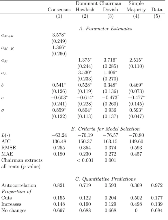
Tables 1 through 6 report empirical results for the monetary committees of the Bank of Canada, the Bank of England, the European Central Bank, the Swedish Riksbank, and the Federal Reserve under the chairmanships of Alan Greenspan and Arthur Burns, respectively. Panel A in these tables reports Maximum Likelihood estimates of the parameters of the interest rate process under each protocol. Although some coe cients are not statistically
signi cant, estimates for all protocols are generally in line with the theory in the sense that they imply that committees tend to raise (cut) interest rates when in ation (unemployment) increases.
Panels B and C respectively compare the protocols in terms of standard model selection criteria and in terms of their quantitative predictions. The latter are computed by means of stochastic simulation as follows. Given current in ation and unemployment and the previous observation of the nominal interest rate, we draw a realization of t from a Normal
distribution with zero mean and standard deviation equal to its ML estimate. Then, for each protocol, we compute the preferred policies of the key member(s) using the ML estimates of their reaction function parameters and use the political aggregators in Section 2 to derive the interest rate selected by the \arti cial" committee. This algorithm is repeated as many times as the actual sample size to deliver one simulated path of the nominal interest rate. Then, we compute the autocorrelation function and the proportion of interest rate cuts, increases, and no changes from the simulated sample. The numbers reported in Panel C are averages of these statistics over 240 replications of this procedure.
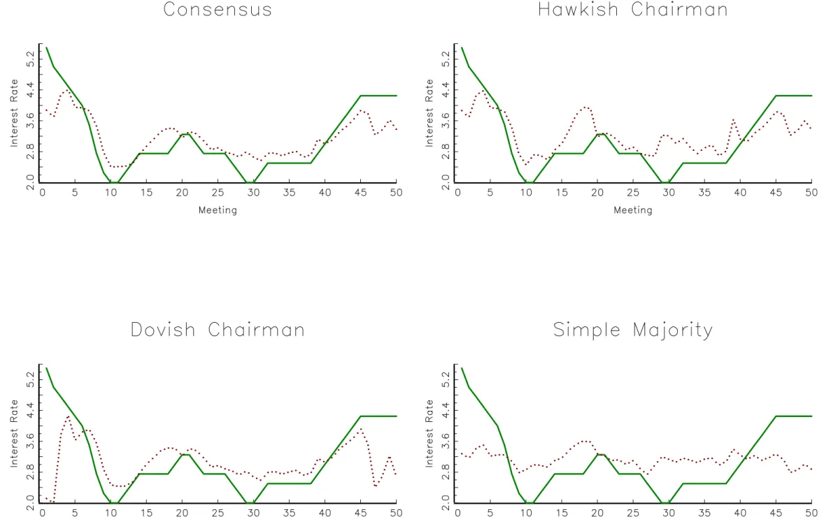
As we will see, results in these two panels show that for all committees in the sample, the consensus model is empirically superior to the other models of collective decision making. Let us start by comparing the consensus and simple-majority models. These two models share the property that no member controls the agenda and primarily di er in the size of the majority required to a pass a proposal. In particular, recall that when the size of the quali ed majority reduces to simple majority, the consensus-based model predicts that the committee selects the median's preferred alternative. Panel B in Tables 1 through 6 shows that for all monetary committees, the simple-majority model features larger Root Mean Squared Error (RMSE), Mean Absolute Error (MAE) and Akaike Information Criteria (AIC) than the consensus model. The comparatively poor performance of the simple-majority model can be seen in Figures 3 through 8, which plot the interest rate decisions and the tted values under all protocols for each committee in the sample. Although the simple-majority model tracks interest rate decisions in broad terms, the quantitative di erence between actual and predicted values is the largest among the protocols studied. There are two reasons for this result. First, the simple-majority model generates interest rate autocorrelation only from the serial correlation of in ation, unemployment and the disturbance term. However, the serial correlation of these variables is not large enough to account for the large autocorrelation of the nominal interest rate. To illustrate this point, Figure 9 plots the autocorrelation functions (up to ten lags) implied by each protocol and the one computed from the data, and Panel C reports the rst-order autocorrelations. From these gure and panel, it is clear that the simple-majority model generally predicts less interest rate persistence than the
consensus model and than found in the data. Second, the simple-majority model delivers a linear reaction function whereby the interest rate changes whenever in ation, unemployment, or the shock realization change. Hence, this model cannot explain the relative large number of instances where the committee keeps the interest rate unchanged despite the fact that fundamentals have changed. From the simulations reported in Panel C, we can see that this model predicts that the proportion of observations where the nominal interest rate remains unchanged is exactly zero, while the consensus model predicts a proportion similar to that found in the data.
These results are consistent with empirical and experimental evidence that committee decisions typically involve quali ed, rather than simple, majorities. For example, the voting records of the committees of the Bank of England, the Riksbank and the Federal Reserve show that split decisions are extremely infrequent. The experimental study by Blinder and Morgan (2005) nds than even though their arti cial monetary committee is supposed to make decisions by majority rule, in reality most decisions are unanimous. Experimental runs of the divide-the-dollar game show that despite the simple-majority requirement necessary to pass a proposal, the agenda setter does not always select a minimum winning coalition: in some cases (roughly 30 to 40 percent of the experiments in McKelvey, 1991 and Diermeier and Morton, 2005), agenda setters allocate money to all players.
It remains an open question why a committee formally operating under simple majority rule adopts a super-majority rule in practice. The search for consensus might be motivated by the belief that split-votes lead to aggrieved minorities and undermine future cooperation. Another explanation is proposed by Bullard and Waller (2004) and Dal Bo (2006), who argue that a super-majority rule may help overcome time-consistency problems by inducing policy-stickiness.18
Now let us compare the consensus and agenda-setting models. These two protocols deliver outcomes di erent from the median policy, predict a time-varying gridlock interval where the committee chooses to keep the interest rate unchanged, and endogenously generate interest rate autocorrelation from the role of the status-quo as the default policy. However, these protocols generate di erent implications for the size of interest rate adjustments. More precisely, the agenda-setting model predicts larger interest rate increases (decreases) than the consensus model when the chairman is more hawkish (dovish) than the median. The reason for this is that the chairman controls the agenda in the agenda-setting model while
18Alternatively, it might be the case that the initial status quo determines a basic form of entitlement.
In a laboratory study, Diermeier and Gailmard (2006) nd that subjects are more willing to accept less generous o ers if the proposer's reservation value is high, thereby supporting the idea that a favorable initial status quo determines an entitlement to a larger amount of resources. In our context, this would explain why a majority of committee members who dislike the status quo are less willing to push for a policy change.
no member does in the consensus model. Hence, deviations from the median's preferred policy are systematically in the favor of the chairman's in the former model.
From Panel B in Tables 1 through 6, we can see that for all monetary committees, the two versions of the agenda-setting model feature larger RMSE, MAE and AIC than the consensus model. The poorer performance of the agenda-setting model in terms of t may also be observed in Figures 3 through 8. Note, in particular, that the agenda-setting model with a hawkish (dovish) chairman tends to overpredict the magnitude of interest rate increases (decreases) compared with the consensus model. In terms of the statistics reported in Panel C of all tables and the autocorrelation functions plotted in Figure 9, it also clear that the agenda-setting models is not as successful as the consensus model in replicating the persistence of interest rates and the proportions of interest rate cuts, increases, and no changes observed in the data.19
Recall that in the setting model with a hawkish (dovish) chairman, the agenda-setter proposes an increase (decrease) of the nominal interest rate to either of two possible regimes depending on whether the acceptance constraint is binding or not. As noted above in Section 3.2, it is not possible to know ex-ante whether this constraint is binding. However, given the ML estimates, it is possible to construct ex-post probability estimates that a given interest rate observation belongs to either regime. We found that in all cases and for all committees in the sample, interest rate increases (decreases) by the hawkish (dovish) chairman are generated by the regime where the acceptance constraint binds. This suggests that even though the chairman has proposal power, he often has to compromise and choose a policy proposal that takes into account the preferences of the other committee members. Based on FOMC transcripts for the period 1987 to 1996, Chappell et al. (2005, p. 186) conclude that \there are at least suggestions that Greenspan's proposals were crafted with knowledge of what other members might nd acceptable."
In the rest of this Section, we investigate in more detail the reasons why the agenda-setting model is less empirically successful than the consensus-based model. A feature of the agenda-setting model is that the chairman is able to use his proposal power to extract all rents when the status quo is su ciently far from the median's preferred interest rate. For example, when it 12 [2iM;t iA;t; iM;t), the hawkish chairman proposes the policy 2iM;t it 1;
which is the re ection point of the status quo with respect to the median's preferred interest
19When we compare both versions of the agenda-setting model, results in the tables show that, except for
the ECB, the version with a hawkish chairman meets somewhat greater empirical success than the version with a dovish chairman. In particular, the former delivers smaller RMSE, MAE and AIC and larger interest rate autocorrelation than the latter. Notice that in both cases the predicted distribution of interest rate changes is asymmetric with proportionally more increases than decreases (decreases than increases) in the hawkish (dovish) case.
rate. The proposed policy leaves the median as well-o as under the status quo and delivers all surplus to the chairman, who has fully exploited his proposal power. In order to test this feature of the agenda-setting model, consider the following statistical model
it= 8 > > < > > : iA;t; if it 1> iA;t; it 1; if iM;t 6 it 1 6 iA;t; (1 + )iM;t it 1; if ((1 + )iM;t iA;t)= 6 it 1 < iM;t; iA;t; if it 1< ((1 + )iM;t iA;t)= : (7)
where 2 (0; 1]. Note that when = 1; (7) is the interest rate process implied by the agenda-setting model with a hawkish chairman. Consider relaxing the restriction = 1 so that now = 1 for a \small" > 0: Then, when it 12 [((1 + )iM;t iA;t)= ; iM;t), the
proposed policy would be (1 + )iM;t it 1 < 2iM;t it 1:20 This means that, given the
status quo, the proposal is now closer to the median's ideal point than under the original protocol and, consequently, the median collects part of the rents. This simple argument suggests that the implication that the chairman uses his agenda-setting power to extract all rents may be statistically tested via a Lagrange Multiplier (LM) test of the restriction = 1. The p-values of this test are reported in the last row of Panel B and indicate that the restriction is strongly rejected by the data from all committees. (A similar argument and test, deliver the same result in the case of the dovish chairman.) Thus, the data reject the strong form of agenda control embodied in the agenda-setting model by Romer and Rosenthal (1978), whereby proposals are made under closed rule (that is, with no counter proposals allowed). It is interesting to note that this result also holds for the FOMC despite the common view that its chairman exerts almost undisputed power and evidence from the transcripts and minutes that other committee members usually do not bring forward counter proposals once the chairman has made his policy recommendation.
In what follows, we test whether the chairman is able to at least partially exploit his proposal power. In particular, notice that if we were to empirically nd a ML estimate of inside the range (0; 1); this would suggest a form of bargaining between the median member and the agenda-setting chairman. On the other hand, if we were to nd that ! 0, then the speci cation (7) would approach the interest rate process implied by the consensus model (with the thresholds appropriately relabeled) where no member controls the agenda. This discussion shows that the speci cation (7) encompasses both the agenda-setting and consensus models and, consequently, provides a mean for directly comparing both models. In particular, one could imagine estimating (7) using actual data and then testing, for example, whether is statistically closer to 0 or 1: We attempted this strategy
20To see this, substitute in = 1 ; write the inequality as (2 )i
M;t (1 )it 1< 2iM;t it 1, and
but found that when the encompassing model was estimated, the ML estimate of would converged to 0 in all cases. Since = 0 is the lower bound of the parameter space, regularity conditions are violated, and standard tests do not have the usual distributions. However, the fact the data strongly prefer 0 compared with = 1 constitutes further evidence against the notion that the chairman is able to control the agenda by excluding some alternatives from the vote. Thus, the existence of an ine cient status quo does not appear to represent a su cient threat that the chairman can exploit to pass a large interest rate change towards his preferred policy. Instead, results suggest that starting, for example, from a low status quo, the committee adjusts the interest rate up to the value preferred by a pivotal member. Our results are in line with laboratory experiments on committee decision making. For example, Eavey and Miller (1984) test the prediction of the agenda-setting model in a one-dimensional policy space and nd that the agenda setter does in uence committee decisions and bias the policy outcome away from the policy preferred by the median member. How-ever, contrary to the strong implication of the model, the agenda setter does not seem to select his most preferred policy from among the set of alternatives that dominate the status quo. Recent experimental studies test the predictions of Baron and Ferejohn's (1989) ex-tension of the agenda-setting model and nd that the individual selected to make a proposal enjoys a rst-mover advantage, as predicted by the theory, but does not fully exploit his proposal power (see McKelvey, 1991, Diermeier and Morton, 2005, Frechette et al., 2005, and Diermeier and Gailmard, 2006). In the empirical literature, Knight (2005) analyzes U.S. data on the distribution of transportation projects across congressional districts. His results support the qualitative prediction that legislators with proposal power secure higher spending in their districts but, in quantitative terms, the estimated value of proposal power is in some cases lower than what is implied by the theory.
Although our ndings reject the notion that the chairman controls the agenda in the strong form assumed by Romer and Rosenthal (1978) and in the weaker form examined above, they do not necessarily imply that the chairman has the same power as his peers. For example, a proposal rule similar to the one in Panel A of Figure 2 may arise from a committee that makes decisions according to the consensus-based protocol plus the requirement that the super-majority must include the chairman.
In summary, a robust nding of this paper is that, among the protocols examined, the consensus-based model describes more accurately interest rate decisions than the alternative models, for all committees in our sample. This means that, in addition to the formal rules under which monetary committees operate, their decision making is also the result of unwritten rules and informal procedures that deliver observationally equivalent policy decisions.
4
Conclusions
To our knowledge, all existing studies that estimate interest rate rules abstract from the vot-ing process that lead to policy decisions. A large body of anecdotal evidence hints instead at the importance of strategic considerations in the decision-making process. Committee members di er along various dimensions and, consequently, are likely to have di erent pre-ferred interest rates. The way committees resolve these di erences crucially depends on the particular voting protocol (implicitly or explicitly) adopted. In this paper, we consider three voting protocols that capture some relevant aspects of the actual monetary policy making by committee: the consensus, the agenda-setting and the simple-majority models. The three protocols have distinct time series implications for the nominal interest rate. These di erent implications are the basis for empirically distinguish among the three protocols using actual data from the policy decisions by committees in ve central banks. A robust empirical conclusion is that the consensus model is statistically superior to the other two voting protocols. This result is observed despite the fact that all central banks (except the Bank of Canada) considered in our sample do not formally operate under a consensus (or super-majority) rule. This result is consistent with a large experimental literature on committee decision making that indicates a preference for oversized or nearly unanimous coalitions even in strict-majority rule games.
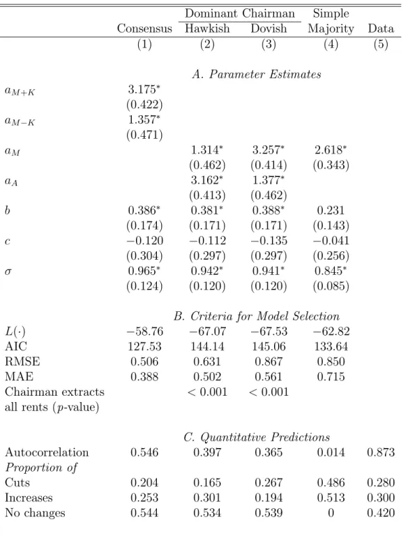
Table 1. Bank of Canada
Dominant Chairman Simple
Consensus Hawkish Dovish Majority Data
(1) (2) (3) (4) (5) A. Parameter Estimates aM +K 3:175 (0:422) aM K 1:357 (0:471) aM 1:314 3:257 2:618 (0:462) (0:414) (0:343) aA 3:162 1:377 (0:413) (0:462) b 0:386 0:381 0:388 0:231 (0:174) (0:171) (0:171) (0:143) c 0:120 0:112 0:135 0:041 (0:304) (0:297) (0:297) (0:256) 0:965 0:942 0:941 0:845 (0:124) (0:120) (0:120) (0:085)
B. Criteria for Model Selection
L( ) 58:76 67:07 67:53 62:82
AIC 127:53 144:14 145:06 133:64
RMSE 0:506 0:631 0:867 0:850
MAE 0:388 0:502 0:561 0:715
Chairman extracts < 0:001 < 0:001
all rents (p-value)
C. Quantitative Predictions Autocorrelation 0:546 0:397 0:365 0:014 0:873 Proportion of Cuts 0:204 0:165 0:267 0:486 0:280 Increases 0:253 0:301 0:194 0:513 0:300 No changes 0:544 0:534 0:539 0 0:420
Notes: The superscripts and y denote the rejection of the hypothesis that the true para-meter value is zero at the 5 and 10 percent signi cance levels, respectively. The proportion of cuts, increases and no changes may not add up to one due to rounding.