Université de Montréal
)%//,
3ZÇ
Phylogenetic Shadowing Using a Model Selection Process
par
Mahshid Shakiba
Département d’informatique et de recherche opérationnelle Faculté des arts et des sciences
Mémoire présenté à la Faculté des études supérieures en vue de l’obtention du grade de Maître ès sciences (IVI.Sc.)
en informatique
Juillet. 2006
C
h
Université
(III
de Montré al
Directïon des bibliothèques
AVIS
L’auteur a autorisé l’Université de Montréal à reproduire et diffuser, en totalité ou en partie, par quelque moyen que ce soit et sur quelque support que ce soit, et exclusivement à des fins non lucratives d’enseignement et de
recherche, des copies de ce mémoire ou de cette thèse.
L’auteur et les coauteurs le cas échéant conservent la propriété du droit
d’auteur et des droits moraux qui protègent ce document. Ni la thèse ou le
mémoire, ni des extraits substantiels de ce document, ne doivent être imprimés ou autrement reproduits sans l’autorisation de l’auteur.
Afin de se conformer à la Loi canadienne sur la protection des renseignements personnels, quelques formulaires secondaires, coordonnées
ou signatures intégrées au texte ont pu être enlevés de ce document. Bien
que cela ait pu affecter la pagination, il n’y a aucun contenu manquant.
NOTICE
The author of this thesis or dissertation has granted a nonexciusive license allowing Université de Montréal to reproduce and publish the document, in part or in whole, and in any format, solely for noncommercial educational and
research purposes.
The author and co-authors if applicabLe tetain copyright ownership and moral rights in this document. Neither the whole thesis or dissertation, nor
substantial extracts from it, may be ptinted or otherwise reproduced without the author’s permission.
In compliance with the Canadian Privacy Act some supporting forms, contact
information or signatures may have been removed from the document. While this may affect the document page count, it does not represent any loss of
Faculté des études supérieures
Ce mémoire intitulé:
Phylogerietic Shadowing Using a Model Selection Process
présenté par: Mahshid Shakiba
a été évalué par un jury composé des personnes suivantes: Alain Tapp président-rapporteur Miklôs Csilrés directeur de recherche Damian Labuda membre du jury
RÉSUMÉ
Le génome humain et les génomes de certains autres primates ont été récemment séquencés ou sont en cours de sécfuençage. Les primates sont d’excellents modèles pour étudier la biologie de l’humain.
La comparaison du génome humain à ceux d’autres primates est d’un très haut intérêt. Cependant, dû à la grande similarité qui existe au niveau des nucléotides entre ces derniers, l’interprétation des résultats des comparaisons entre génomes voisins constitue encore un grand défi. La méthode de “shadowing phylogénéticue” a été largement utilisée dans la prédiction de la fonction des régions non codantes. Cette méthode utilise principalement l’approche de la fenêtre coulissante ou bien un modèle de Markov caché qui permettent tous les deux de détecter les régions
sous sélection négative.
Ce mémoire présente une nouvelle approche dans la prédiction de régions fonc tionnelles dans trois génomes voisins. Dans cette approche nous ne faisons aucune hypothèse quant à la distribution des régions conservées dans le génome. Nous uti lisons le principe de la “description de longueur minimale” (MDL) provenant de la théorie de l’information. Cette stratégie permet, non seulement, la prédiction de
régions du génome qui se trouvent être sous la sélection négative, mais aussi celles sous la sélection positive. Cela peut s’avérer très utile puisque ces dernières régions définissent souvent les traits biologiques particulier. Notre approche a été testée en utilisant les données de simulation et les alignements multiples des trois séquences
génomiques de l’humain, du chimpanzé et du babouin.
Mots clés: Génomique Comparative, Ensemble de Segments de Plus Hauts Scores, Sélection de Modèles, Shadowing Phylogénétique.
The genomes of human and a few nonhuman primates have been sequenced and more genomes of primates will be completed in the near future. Nonhuman pri mates are the rnost pertinent organisms to comprehend human biology.
There lias been a considerable interest in comparing the human genome with the nonhuman primates. However, due to the high degree of similarity between primates at the nucleotide level, interpreting the resuits between closely related genomes is very cliallenging. Phylogenetic shadowing lias been a widely utilized method in predicting functionality in non coding genomic regions. The main method in phylogenetic shadowing is either a siiding window or a Hidden Markov Model that can detect the regions under negative selection in closely related genomes.
This thesis presents a novel approach to predict functional regions in three closely related genomes. This method does not make any assumptions about the underlying distribution of conserved regions. We use instead an information the oretic approach based on minimum description length. In addition to predicting negative selection, this strategy is used to identify regions under positive selection. Regions under positive selection are likely to determine unique biological traits of species. This approach is tested both on simulated data and on a multiple align ment of human, chimpanzee and baboon genomic sequences.
Keywords: Comparative Genomics, Maximum-Scoring Segment Set, Model Selection, Phylogenetic Shadowing.
CONTENTS
RÉSUMÉ iii
ABSTRACT iv
CONTENTS y
LIST 0F TABLES vii
LIST 0F FIGURES viii
LIST 0F ABBREVIATIONS ix
NOTATION x
DEDICATION xii
ACKNOWLEDGEMENTS xiii
CHAPTER 1: INTRODUCTION f
1.1 A Short Review of Biology 1
1.2 Evolution and Comparative Genomics. . . 3
1.3 Phylogeny and Evolutionary Trees 5
1.4 Sequence Alignments 8
1.5 Comparative Genomics and Phylogeny 11
CHAPTER 2: PHYLOGENY IN PROBABILISTIC FRAMEWORK 16
2.1 Maximum Likelihood 17
2.2 Models of Sequence Evolutions without Gaps 18
2.3 Likelihood of a Tree 22
2.3.1 Estimation of IViodel Parameters 25
CHAPTER 4: RESULTS... 4.1 Simulation
4.1.1 Simulation Resuits 4.2 Real Dataset (CFTR Region)
CHAPTER 5: SUMMARY AND CONCLUSION
5.1 Conclusion 5.2 future Work BIBLIOGRAPHY 77 77 79 2.4.1 Phylogeny and Missing Data
2.4.2 Tree-Hidden Markov Model 2.5 Phylogenetic Analysis Tools
CHAPTER 3: METHODOLOGY
3.1 Maximum Likelihood Estimate of Segments
vi 27 2$ 33
3.2 Model Parameters
3.3 Estimating the IViodel Parameters 3.4 Optimization I\’Iethod
3.4.1 Powell’s l’Iethod 3.5 false Positive Rates 3.6 Application Description 3.6.1 Input file . 3.6.2 Output File 3.6.3 Options . . . 3.6.4 User Interface 4.2.1 4.2.2
Regions under Purifying Selection Regions under Positive Selection
LIST 0F TABLES
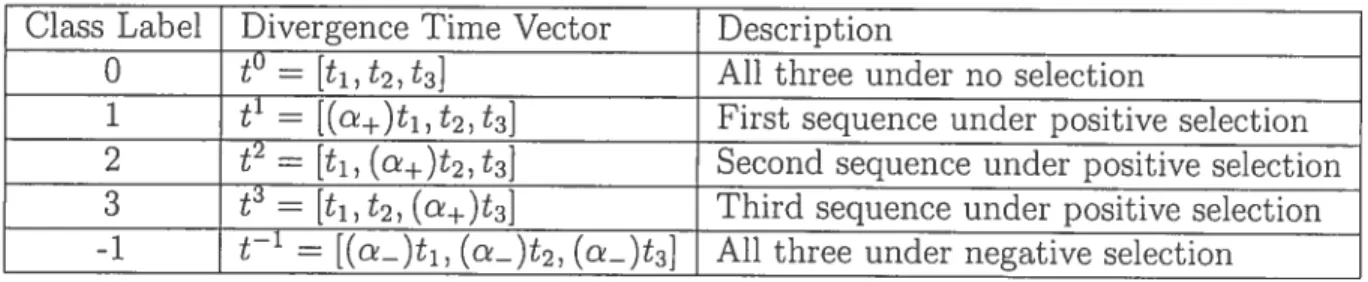
3.1 Labels and divergence tirne vectors for coftimn classes 38 4.1 Transition and ernission probabilities used in generating a sequence
under the tree-HMM model 59
4.2 Average of segmentation error (N = 10, 000) 60 4.3 Relative error of model parameters with standard phylogeny model
(N= 10,000) 61
4.4 Relative error of model parameters with tree-HMM model (N =
10, 000) 62
4.5 Average of segmentation error (N 100, 000) 63
4.6 Relative errors of model parameters with standard phylogeny model
(N = 100, 000) 63
4.7 Relative errors of model parameters with tree-HMM moclel (N =
100, 000) 64
4.8 Average of segmentation error for each class using standard phy
logeny model (N = 100, 000) 66
4.9 Maximum, minimum, median and average length of the regions pre
dictecl to be under selection 70
4.10 MDLShadow predictions overlapped with previously identified ul
traconserved regions 72
4.11 Unannotated regions predicted to 5e under negative selection 73 4.12 Positive selection regions with more than 20% mutations in human
1.1 DNA structure 2 1.2 Phylogenetic tree for species rat, mouse and rabbit 6 1.3 An example of phylogenetic tree; rooted tree (a), unrooteci tree (b) 7 1.4 Examples of homolog, ortholog and paralog genes 9 1.5 Use of genome comparisons at varions evolutionary distances to an
notate the human genome 14
1.6 Primate phylogenetic tree 1.5
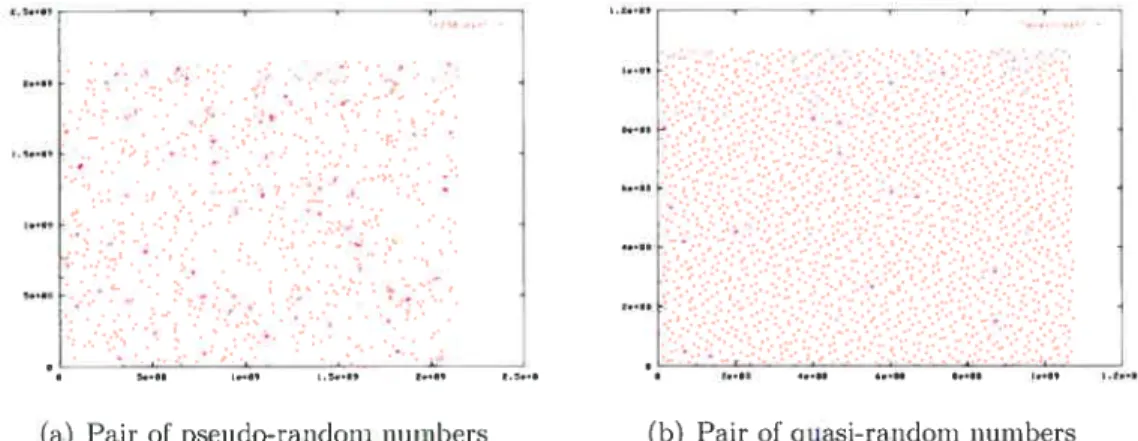
2.1 Overview of calculating the likelihood of a given phylogenetic tree 23 2.2 A short tree-HMM for a simple tree with two nodes 29 3.1 Scatter plot of the pair of sequences generated by pseudo-random
generator (a), quasi-random generator (b) 46
3.2 Screenshot of the main menu 52
3.3 Screenshot of the “Run” dialog 52
3.4 Screenshot of the “Options” dialog 53
3.5 $creenshot of UCSC genome browser with the predicted regions as
a custom track 55
4.1 Segmentation error for segments of different lengths with different
penalization factors 65
4.2 Annotation for CfTR region displayed as a user suppÏied track on
UCSC genome browser 68
4.3 Convergence of the estirnated parameters and segmentation for the
CFTR region 69
4.4 Composition of conserved elements hy annotation types 71 4.5 A conserved intronic region of 5T7 displayed on UC$C genome browser 74 4.6 Composition of regions predicted to be under positive selection by
LIST 0F ABBREVIATIONS
A Adenine
AIC Akaike Information Criterion AR Ancestral Repeat
bp Base Pair
BIC Bayesian Information Criterion C Cytosine
DD Delete-Delete Transition in Tree-HMM DM Delete-Match Transition in Tree-HMM DNA DeoxyriboNucleic Acid
G Guanine
GFF Gene-Finding Format or General Feature format HMM Hiden Markov Model
LLR Log-Likelihood Ratio
MD Match-Delete Transition in Tree-HMM MDL Minimum Description Length
ML Maximum Likelihood
MM Match-JVlatch Transition in Tree-HMIVI My Million Years
ORf Open Reading Frame RNA RiboNucleic Acid
n Number of taxa
X Alignrnent of DNA sequences N Length of alignment
X ith column of alignment Pr(a) Probability of a
T Topology of the phylogenetic tree
Maximum likelihood estimate of phylogenetic tree
t Number of mutations along the brandi connecting jth sequence to its ancestor
Nucleotide base at position i in jth sequence of alignrnent
Q
Instantaneous substitution rate matrix,i IVIean instantaneous substitution rate nA Equilibrium frequencies of Adenine
no Equilibrium frequencies of Cytosine n0 Equilibrium frequencies of Guanine n7-’ Equilibrium frequencies of Thymine P(t) Substitution probability matrix
R Ratio of transition to transversion E() Emission of sequence x at position j
M(r) Transition of sequence x from tic match state or * if x does not
use match state at position i
D(x) Transition of sequence r from tic delete state or * if r does not use
xi
7rMM Prior probability of Match-I\’Iatch transition n Prior prohability of Match-Delete transition
7CDD Prior probability of Delete-Delete transition 7TDM Prior probability of Delete-Mat.ch transition
r Rate constant in match-transition matrix ‘u Rate constant in clelete-transition matrix $ A segment
ç5 A partition
ç5 Size of the partition ç5 w(ç5) Score of the partition ç5
(ç5) Complexity-penalized score of the partition ç5
Z Labels of each column of alignment after segmentation C Number of classes
z Inclicator variable of column i for class c
c+ IVlutation rate of the regions under positive selection
o Mutation rate of the regions under negative selection t Divergence tirne vector for class c
w Log-likelihood ratio of column i being in class c versus being in neutrally evolving class
d Number of variables needed to specify a partition À Penalization factor
Wc(i) Score of the optimal partition for prefix [1, j] that ends with a seg ment labeled c
$egtoi Tolerance parameter which controls the convergence of segmenta tion
ftot Tolerance parameter which controls the convergence of Powell’s metho d
ACKNOWLEDGEMENTS
first, I would like to express mysincere gratitude to mysupervisor Professor I\’Iiklôs Csfirds for bis valuable guidance patience, constructive comments auJ friendly manner throughout the course of this research. This researcli would not have heen possible without bis supervision and support.
I am indehted to André Caron, rny former boss at SignalGene Tue, for introducing me to ffeld of bioinformatics.
On a personal basis, I am very grateful to rny parents. No words can truly ex press my deepest auJ sincere appreciation for ail they have donc for me.
Last but not least, I would like to thank my husband, Behrouz, for bis under standing, love and continuous moral support.
INTRODUCTION
1.1 A Short Review of Biology
Biology is the science that studies living organisms, their structures, functions, origins, and evolution. The number of currently existing species is estimated to be in the order of i0 (Lynch 2006). Ail organisms are made of the same unit of
life, the ceit which lias ail the essential information and mechanisrn for its growth, maintenance and reproduction (Hunter 1993). Some organisms like yeast have a single ceil. IViulticellular organisms have different ccli types. There are two major
categories of orgauisms: eukaryotes and prokaryotes. Virtually every eukaryotic ceil contains a nucleus, defined as an area of the ceil that holds the genetic material. The nucieus is separated by membranes from the rest of the ccli. Organelles such as mitochondria and chloroplasts are specialized cellular structures of eukaryotes. Prokaryotes do not have nuclei and organelles.
The genetic materiai is deoxyribonucleic acid, abbreviated as DNA. DNA eau 5e linear (in eukaryotes and in some prokaryotes) or circular (in rnost prokaryotes) (Tamarin 1999). The genetic material of eukaryotes is organized into chromosomes. Each chromosome contains a double-stranded DNA molecule, along with a nurn ber of proteins. Sexually reproducing organisms have a paternal and a maternai chromosome for every chromosome. These organisms are ca.lled diploids. for in stance, human cells are diploid, and contain 22 pairs of chromosomes (so-cailed aut.osomes), as well as two sex chromosomes.
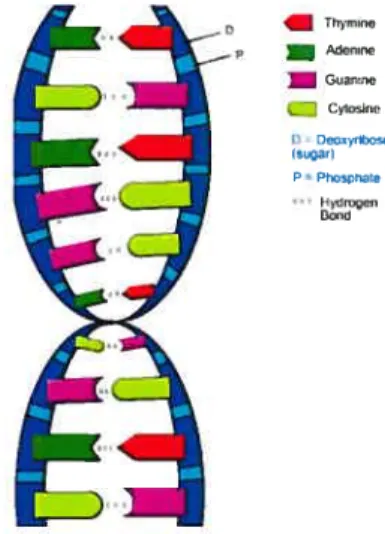
DNA has a double helix moiecular form hke a twisted ladder (Watson and Crick 1953). $ugar and phosphate units make up the backbone of helices. Each back bone unit has a nitrogenous base and these bases make the “rungs” of the ladder. Normally, four types of bases are found in DNA: adenine, thymine. guanine and cytosine. Adenine and guanine nucheotides are purines and cytosine and thymine
2 are pyrirnidines. Figure 1.1 illustrates the structure of the DNA.
Thyrse p — Meflrrw Guanne Cytosino O 000ayribose (nstgar) P=Phosphate Hyd,oçen Pond
The four bases are abbreviated hy the letters A. T, G and C and are concate nated into a sequence to represent a DNA molecule (e.g. CGGTTAC). There is no restriction on base types locatecÏ on one straid. However, there is a restriction on the hases paired on opposing strands. If aclenine is the base of oiie strand, the other must be thymine; if one base is cytosine. flic other shoulci he guanine. Tius relationship is caÏled comptementarity (Watson and Crick 1953). Complementary nature of base pairs makes the duplication of DNA an accurate process. The dou ble helix “unzips” and each strand provides a template to create a new straud of DNA. This process resuits in two double helices exactly like the first. These base pairs are kept to each other hy hydrogen bonds. The length of DNA is usually rneasured in the unit of base pairs (bp).
Functional tasks in a
ecu
are mostly carried out by proteins (Hunter 1993). Hu man being is likely to have more than 100, 000 different kinds of proteins. Proteins are macromolecules that are made of the many combinations of 20 arnino acids. Long proteins may consist of up to 4500 amino acids. This makes the space of ail possible proteins structures very large: 204500 or 105850. However, most of proteinsare 10 times smaller. Proteins fold up to make specific three-dimensional fornis. Figure 1.1: DNA structure (from fliologyCorner)
Biochemical functionality of proteins depends on their amino acid compositions and their three dimensional shape. Primary structure of a protein is the seciuence of arnino acids that makes a specific protein and is coded in DNA by sequence of nucleotide triplets. Each triplet of nucleotides is called a codon and corresponds to an amino acid. There are 43 = 64 possible codons. Three of these codons specify the end of a protein sequence and are called stop codons. Other codons code for the 20 amino acids. Hence, the same amino acid can 5e encoded by several codons. For instance, alanine is represented by codons GCT, GCC, GCG and GCA. There are three possible places to start transiating a strand of DNA sequence into amino acids. Each of these parsing is called a reading frame. If a reacling frame is long enough and does not have a stop codon in the middle is called open reading frarne or ORF and it can be translated into a protein. Since eacli strand of DNA can be parsed, therefore, there are six reading frames for every DNA sequence.
In most eukaryotes. the stretch of DNA sequence that codes a single protein lias some non-coding sequences inserted into them. These non-coding sequences are called introns and are spliced out before a sequence serves as a template for protein synthesis (Gilbert 1978). The stretcies of DNA that are transiateci into amino acids are called exons. In addition to the coding sequence of proteins, DNA encodes some other information. Every cell in the body has the same DNA but each cell type produces different set of proteins and in different quantities. The DNA signals specify where a protein should start and end; where spiicing of intron should occur; how much of each protein should 5e synthesized. These signals are regulatory elements and are referred to as non-coding functional regions.
All the genetic material of an organism is called its genome. Gene is the discrete functional unit of genetic material and codes for some products (RNA or protein).
1.2 Evolution and Comparative Genomics
Evolution is the keystone paradigrn in biology. Organisms reached their cur rent state through evolution. The similarity of molecular rnechanisms in living
4 organisms is explained by a common ancestry.
An evolutionary process lias three elernents: inheritance, variation and selec tion. Inlieritance is tlie transfer of characteristics of parent to offspring. Almost ail of tlie structure and function of an organism is passed by inheritance. Tlie amount of variation between generations is limited and is related to tlie size of the population (Hunter 1993).
Variation in the inherited material is essential for evolution. Variation is defined as the process tliat make offspring different from their parents. When some of the bases in a genome are clianged or a longer piece of a genome is duplicated or removed, a mutation occurs. Mutation in hereditary material is one of several possible sources of variation (Hunter 1993). Evolutionary changes by mutation are very slow because most of tlie mutations are deleterious or neutral. $exual recombination is another source of variation.
Natural selection favors tlie organisms that have aclvantages and are better adapted to tlieir environment. Therefore, if the generated variant lias an advantage, then tliese changes propagate througli the population with a certain probability (Kimura 1968). This probability is determined by the relationship between the size of the population and the effect of the mutation; small aclvantages in large populations do not tend to hecome fixed. In contrast, srnall disadvantages in srnall populations may become fixed.
Tlie similarity between living things is the result of inheritance from a common
ancestor; the variety comes from the variation and selection elements of evolution (Hanter 1993).
Recently, it lias become possible to determine the genome sequence of species. Genornics, tlie most recent branch of biology, studies genomes. The size of the genome varies between organisms. The liuman genome consists of about 3 x iO base pairs (Lander et al. 2001).
The focus of tlie next phase of the Human Genorne Project is to find ail the functional regions of genome sequences (Hardison 2003). Analysis of the individual genome sequences helps to understand the genome structure but it is not very
informative about genome functions (Milier et al. 2004). Comparative analysis of genome sequences lias been and xviii be a major approaci to icIentify functional regions of each genome (Miller et ai. 2004).
It is known that functional sequences are subject to evoiutionary selection (Milier et al. 2004). Mutation in functionai regions lias usualiy deieterious effect on the organism. Generally, mutations in non-functional regions do not have any effect on the procreative fitness of an organism and xviii accumulate over tirne (Kirnura 1968). That is the reason functional sequences change more slowly than the non functional sequences. These regions are referred to be under negative or purifying selection. Non-functionai regions are sometirnes referred to as neutral evoiving re gions. However, there might be a shght selective pressure on non-functional regions as weH. It is estimated that about 5% of human genome is under purifying selection (Miiier et ai. 2004); within this subset, 1% to 2% encodes proteins (IViargulies et ai. 2003).
Positive seiection, in contrast, causes sequences to change faster. These regions are often responsibie for bioiogicai differences between organisms. Positive seiection is sometimes referred to as Darwinian selection. Que of the aims of comparative genornics is to identify these regions in different genomes. However, predictions about positive and negative seiection regions need experimentai tests to verify their importance and their functionai roies (Miiier et ai. 2004).
1.3 Phylogeny and fvolutionary Trees
Based on the evoiution theory, any set of species are reiated to each other. The more reiated two species are, the more recentiy they diverged from their common ancestor. Understanding the ancestry of the species compared and their relation slip is central to many applications of comparative genomics.
Phylogeny studies the reiationships between organisms and aims (1) to infer the evolutionary hnks between organisms and (2) to estimate the time when they shared a common ancestor (Durbin et ai. 1998).
6 Comparative genornics employs phylogeny in order to understand the genomes of different species and to analyze their differences (Mount 2001). At the saine time, a.s new genome sequences and rnethods to analyze these sequences becorne available, our understanding about phylogeny improves.
Traditionally, morphological characters such as beak shapes or number of legs have been used to infer the phylogeny. Recently, molecular data like DNA sequences and protein sequences are mostly used for this purpose (Mount 2001).
The evolutionary relationships of a group of organisms is represented by a phy logenetic tree (Eriksson 2004). A phylogenetic tree is a connected. acyclic graph, which directs ail edges outward from a designated node, root. In other worcis, it is an arborescence. A phylogenetic tree is an unordered tree. Organisms under coin parison are called taxa. A tree is composed of outer leaves representing the taxa or terminal nodes and nodes and branches representing the relationships between them (Mount 2001). The brandi points within a tree are cailed internai nodes. These nodes are the hypothetical ancestral units and they are used to group exist ing units. The branching reiationships between taxa show how they are related to each other.
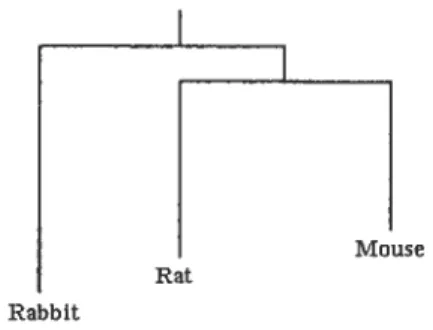
Figure 1.2: Phylogenetic tree for species rat, mouse and rabbit
The tree in Figure 1.2 shows two occurrences of speciation: first the hneage of rabbit had diverged, then the divergence between mouse and rat happened. Usu aliy, the branch length represents the amount of time elapsed since the speciation from a common ancestor but in this figure the scale is not representative.
Rabbit
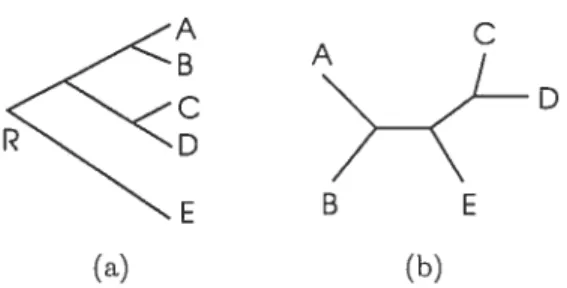
study. Most phylogenetic inference methods are not informative about the position of the root. An example of a rooted tree is shown in Figure 1.3(a). In the rooted tree, an evolutionary path is defined as the path from root to a nocie. In the unrooteci tree, reiationships among taxa are specified but the evolutionary paths are not depicted (Fig. 1.3(b)).
D
(a)
Figure 1.3: An example of phyiogenetic tree; rooted tree (a), unrooted tree (b) (from $ingh 1999).
The topology of a tree is the branching pattern of a tree auJ is denoted by symbol T. In a binary tree, every internai node has two offspring if it is a rooted tree, or 3 neighbors if it is an unrooted tree. In this thesis, trees are assumed to be binary. This assumption about the tree topoiogy is not restrictive because every tree can be approxirnated by a binary tree with very short branches (Durbin et al. 1998).
A rooted tree with n ieaves has n— 1 internai no des. This gives 2n — 1 nocles in
total. Leaves are labeled. The total number of edges is 2n — 2. An unrooted tree
with n taxa lias 2n— 2 noUes and 2n—3 edges. Any unrooted tree can be changed
to a rooted tree by placing a root on any of its edges. Therefore. for a given number
of n ieaves, the number of rooted trees is (2n — 3) times the number of unrooted
trees (Durbin et ai. 1998). The total number of possible unrooted, iabeled binary
B E
8 trees with n leaves is (Felsenstein 2004):
3(n)
=
fl
-5) (1.1)Tire length of each branch cari represent tire number of mutations that occurred in that branch or it cari indicate tire evolutionary tirne passed along tire branch.
Several rnethods are availahie in tire literature to infer tire phylogeny from a given set of sequences. The next chapter discusses phylogenetic inference methods in more details.
1.4 Sequence Alignments
A main use of sequence comparison is to investigate if sequences are related. Tins is usually doue by first aligning tire whole or parts of tire sequences in ciuestion. Sequences cari be aligned across their entire iength (global atignrnent) or only in sorne regions (tocat atignment).
Sequence alignment algorithms are looking for proof that sequences under study have diverged from a common ancestor through mutation and selection processes (Durbin et al. 1998). If they have, they are defined as homoÏogs. Homologous sequences are either orthotogs, paTaÏogs, or enoÏogs. Genes winch are derived from a single gene in the last common ancestor of tire sequences under study, are orthologs (Koonin 2005). Genes winch are related by duplication event are paralogs. Two genes are xenologs if at least one of them is acquired by interspecies horizontal transfer of genetic material. In Figtire 1.4, early globin gene is duplicateci and ri
and /3 globin genes are fornred. ri globin genes in mouse, frog auJ chicken are
orthologs. ri and
/3
globin genes in mouse are paralogs.Substitutions, insertions and deletions are tire basic mutational processes, winch are considered in rnost alignment methods. Substitutions change nucleotides in a sequence; insertions auJ deletions add or remove nucleotides. Insertions auJ deletions are described as gaps (Durbin et al. 1998).
sequence 1: sequence2: sequence3: sequence4:
orthoIo2s aralogs orthologs À.____
r -‘
-
-froΠchickCx mouseCL mousej3 chickj3 frogf3
(X-chain genc f3_chaingdne ne duplic’itipn
darlv g1ot,n gene
TGG GGG ATG CGG - - - C - - - C - - - T GCGT
The quality of the resulted alignment is specifled by an alignment score. Using this score, the next step is to decide whether that aligilment is the resuit of se quences kinship. or it happened by chance (Durbin et al. 1998). The result.s of any comparative method depend on the quality of the underlying alignments used as inputs. To this end, the choices of alignrnent methoci and the scoring system used to evaluate the aligilments are very important.
Two types of alignrnent algorithms have been generally useci in sequence anal ysis (Yu et al. 2002). The first category looks for the optimal allgnment (e.g. $mith-Waterman 1981 algorithm). The second type has a probabilistic nature (Yu and Hwa 2001) and searches for the rnost tikely alignrnents (e.g. pairwise hidden Markov models).
homologs
Figure 1.4: Examples of homolog. ortholog and paralog genes (from NCBI)
Here is an example of an alignment of four sequences. The colurnns in the alignment are also referred to as sites.
CA- TCC
CA- TCC
G- - CGC
10 In the optimal alignment algorithms, a cost is a.ssigned to each kind of substi tutions. Those mutations that are more common will get a smaller cost compared to the less frequent ones. For example, transitions, the substitution of purine-to purine or pyrimidine-to-pyrirnidine, are more freciuent than transuersions, which alter the type of nucleotides (Kimura 1981). Hence, transitions are penalized less than transversions. Biologically, deletions and insertions are more likely to occur as a consecutive group rather than to be scattered discretely and therefore, gaps are usually penalized using affine functions. This means that a cost proportional to the length of the gap is added to a cost for opening a gap. The optimal alignment of sequences seeks to minimize the total cost of nucleotide substitutions, insertions and deletions. For more information about these algorithms refer to Jones and Pevzner (2004).
The second type of alignment algorithms are based on a probabilistic frame work. These methods assign probabilities to alignments and can be used to train a model on data and to obtain model pararneters (Nielsen 2005). The alignment score is usually related to the likelihood of the alignment in a particular proba bilistic framework. The resulting probabilistic model can be used to assess the quality of the alignment or to examine other possible alignments. By assigning probabilities to ah alternative alignments, the similarity between seciuences can be assessed without relying on any specific alignment (Durbin et al. 199$). Only few of these statistical ahignment rnethods take into account the underlying phylogeny of sequences and the likelihood that these sequences have evohved from an unknown root is calcuhated. The most probable alignment along with the model parameters can be obtained using likelihood maximization or Bayesian techniques (see Durbin et al. 199$; Nielsen 2005).
There are several multiple alignment tools available. Among them aie MLA GAN (Brudno et al. 2003), MAVID (Bray and Pachter 2004), DIALIGN (Mor genstern 1999), CLUSTALW (Thompson et al. 1994) and MUSCLE (Edgar 2004). MLAGAN and MUSCLE align DNA and protein sequences respectively. MAVID, DIALIGN and CLUSTALW can be used to align both DNA and protein sequences.
1.5 Comparative Genomics and Phylogeny
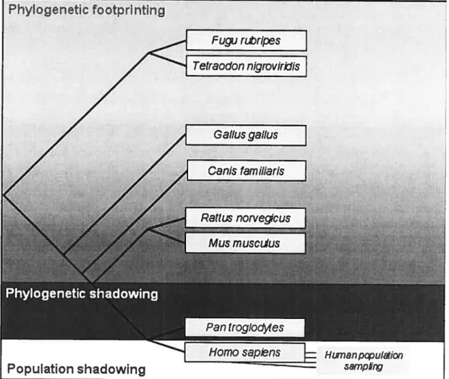
The first problem in comparative genomic studies is the choice of species for analysis (Nobrega and Pennacchio 2003) and it has two steps (Pardi and Goidman 2005). First, a range of species are chosen. This selection is based on the biology these species must share. The second step is to choose some of them for analysis and is usually based on maxirnizing the evolutionary distailce between them. The less similar the sequences are, the easier is to discriminate ftmctional conserved regions from neutrally evolving regions. Figure 1.5 shows the rnethods of comparing genomes at different phylogenetic distances.
Comparisons of distantly related genomes have been widely used to identify shared functionally conserved regions of genornes (Boffelli et al. 2003). For example, the evolutionary distance between human and mouse makes them good candidates for the identification of shared functionally conserved sequences. Since the last time they shared a common ancestor (about 80 million years ago), a large fraction of nucleotides have been changed. However, one can find sirnilarity even between neutrally evolving sequences. These significant changes make it easy to identify functionally conserved regions (Boffelli et al. 2003).
Phylogenetic footprinting (Tagle et al. 1988) is a technique that uses multi species sequence alignrnent to identify highly conserved elements in distant species. $ince functional regions evolve much siower than nonfunctional sequelices, the dif ference in mutation rates in functional and non-functional regions makes it possible to distinguish these regions from each other. This is achieved by comparing the orthologous regions of related distant species. If these regions have well conserved sequences, it is likely that they are functional (Blanchette et al. 2002).
Comparing distant species cannot identify the recent changes in DNA sequences responsible for primate biological traits (Boffelli et al. 2003). For instance, 20o of human functional elements do not have mouse orthologs (Nobrega and Pennacchio 2003). Therefore, comparison of the human sequence to that of other primates is needed. Figure 1.6 shows the phylogenetic tree of primates. Due to their short
12 divergence time tapes 6 to 14 My, Old World monkeys 25 My, New World monkeys 40 My), there is not enough sequence variation between human and other primates (Boffelli et al. 2003). I\/Iore than 90% of human DNA is sirnilar to that of primates (Ovcharenko et al. 2004).
In pairwise comparisons, the lack of sequence variation makes the discrimination of functional from nonfunctional sequences difficuit (Boffelli et al. 2003). Consid ering more species and comparing the genomes of multiple primates can overcome this issue.
Phylogenetic shadowing analyzes the genomes of closely related species anci consiclers the phylogenetic relationship of these species. This approach was flrst used hy Boffelli et aI. (2003) to identify cocling and non-coding functional regions. Sequences from a set of 18 primates. which had a known exon, were used to estimate the mutation rate of the “conserved” and “non-conserved” regions. They found
that the mutation rate for the non-coding regions was 7.3 times higher than the
mutation rate of coding regions. They analyzed four genomic intervals with a known exon. Their resuits show that exon-containing segment lias the smallest cross-species variation.
The interspecies comparison lias the limitation that it can only 5e used to identify functional regions that are responsihie for shared biological traits ancl it cannot reveal the features that are unique to a species. Boffelli et al. (2004) tested the use of population shadowing on sequences of the same species. However, this method needs a very large number of sequences from the individuals of the sanie species. This approach may be more feasible in the near future when large-scale resequencing becomes less costly.
Ovcharenko et al. (2004) developed eShadow, which is a computational tool
for the identification of regions under negative selection through multiple sequence alignments of closely related genomes. e$hadow applies phylogenetic shadowing and allows dynamic visualization of conservation profile of the genomes. eShadow can 5e applied to analyze distant geliomes (e.g. human and mouse), as well as close genornes (e.g. two primates).
One of the prediction method used in eShadow is a two-state hidden Markov model. Ovcharenko et aI. (2004) modeled the distribution of matches and
mis-matches in slow and neutral evolving regions with an HMM. The HMM parameters
can either 5e obtained from a training dataset or 5e optimized using Baum-Welch
algorithm (see Durbin et al. 199$).
eShadow, is the only existing phylogenetic shadowing tool, but it has a few drawbacks. First, it assumes that the distribution of slow and neutral evolving sites follows an HMM. However, there is no evidence in literature that supports
the idea of modeling these regions with an HMM. Second, it can only identify the
regions under negative selection, and positive selection regions cannot 5e iclentified. Positively selected regions are among the most interesting parts of a genome (Miller et al. 2004). These regions are likely responsible for unique traits of each species. It
is with these considerations in mmd that we have developeci a probabilistic frame
work that allows the identification of regions under purifying selection, as well as positive selection in three closely related species. In this framework, no assurnp
tion is required about the distribution of slow, neutral and fast evolving regions. The model parameters along with the annotation of sequences are calculated 5v a maximum likelihood method.
14 Phylogenetic footprinting Gallus gallus Canis familiaris Rattusnoniegcus •‘• Mus musciius Population shadowing Homo S8flS jz HLrnanpcpulelioi — s9mpk%’
Figure 1.5: Use of genome comparisons at various evolutionary distances to an
notate the human genorne. $haded areas representing different methods underlay
a phylogenetic tree of selected vertebrates. In this figure, hurnan (Homo sapiens) genome is compared with the chirnpanzee (Pan troglodytes), mouse (Mus muscu
lus), rat (Rattus norvegicus), dog (Canis familiaris), chicken (Gallus gallus), and fish (Fugu rubripes and Tetrao don nigroviridis) genomes (from Miller et al. 2004).
-J
>NewworId
monkey
,01d-world
m onkeys
}
Figure 1.6: Primate phylogeuetic tree. As a reference, prosimians’ ami rodents’ age is also shown (from Boffelli et al. 2003)
CHAPTER 2
PHYLOGENY IN PROBABILISTIC FRAMEWORK
In many comparative genomics applications, as we emphasized, it is crucial to understand the evolutionary history of the compared species, or, in more general terms, their evolutionary relationships. To this end, it is important to infer the evolutionary tree topology and timelines (represented by the branch lengths) from the observed data.
Inferring a phylogeny is an approximation procedure which aims to provide the best estimate of an evolutionary history based on the information in the data (Hillis et al. 1996). The statistical and computational aspects of phylogeny reconstruction have been introduced about 40 years ago while phylogenies had been around for more than 140 years (Felsenstein 2004). There are several methods to infer the phylogeny of the sequences under study. Most of these methods use alignments computed in a preparatory step for phylogeny construction. They generally start with a multiple alignment of n sequences (representing n terminal taxa), and re turn one or more binary trees describing the evolutionary relationships arnong the sequences. The returned tree (or trees) is produced typically by maximizing some established objective function. The methods can be classified by the nattire of their objective function into three main categories. Namely, distance-based, parsimony and maximum tikeÏihood rnethods. Maximum likelihood approach is the one ap plied in this thesis. For more information about other methods used for inferring phylogenies see Hillis et al. (1996).
Most current approaches in sequence analysis treat alignment and phylogeny separately, although they are intimately linked (Nielsen 2005). Any error in the alignment can lead to a corresponding error in the identification of the tree (Mitchi son 1999). At the same time, aligning DNA and protein sequences is based on the theory that aligned bases are derived from a common ancestor. For this rea son, there are methods that perform alignment and tree-building simultaneously.
Notably, the models presented by Thorne, Kishino, and Felsenstein (1991, 1992) known as TKFÏ and TKF2, and that of Mitchison and Durbin (1995), known as tree-HMM, estimate evolutionary history anci alignrnent scenario at the sanie time (Nielsen 2005).
Maximum likelihood estimates, for seciuence evolution and phylogenetic trees, are the basic mathematical tools in our methodology. The rest of this chapter is dedicated to introduce these concepts.
2.1 Maximum Likelihood
Maximum Likelihood is a statistical procedure which is used to estimate the pararneters of the model that best describes a given dat.a set (Nielsen 2005). For a given data, an analytical function is defined which is the probability of getting that particular set of data under a known model. Maximum likelihood estimates of model parameters is the set of parameter values that maximize the probability of the data.
Inferring pliylogeny using maximum likelihood is achieved by evaluating dif ferent hypotheses about the evolutionary history of the underlying species. The prohability that an explicit model of evolution and the hypothesized history would generate the observed data is calculated. It is assumed that a history with a higher probability to generate the ohserved data is better than the one with a lower prob ability of generating the observed data (Hillis et al. 1996).
Maximum likelihood estimation was flrst applied in phylogenetic inference by Cavalli-Sforza and Edwards (1967). Felsenstein (1981) applied maximum likelihood framework to DNA sequences, and developed the essential computational tools to infer the phylogeny of related species. Later, maximum likelihood was also applied to amino acid sequence data (Kishino et al. 1990; Adachi and Hasegawa 1992).
In order to apply the maximum likelihood method, a model of evolutionary process that accounts for the changes of one sequence into another is required. The model can be completely defined or it may have a few parameters left to
1$ be estimated. A maximum likelihood approach evaluates the probability that the given evolutionary model and the tree topology generated the observed data; the tree that corresponds to the highest likelihood is defined to be the phylogenetic tree of the sequences under study (Hillis et al. 1996). The probability that the tree corresponding to the highest likelihood is the true topology of the taxa at hand increases as the length of alignrnent gets longer. This means that if sequences at terminal nodes are long enough, ML bas a solution for the truc tree topology of these terminal nodes; therefore the maximum likelihood method is statistically consistent (Chang 1996).
2.2 Models of Sequerice Evolutions without Gaps
An explicit model of sequence evolution is needed to calculate the likelihood of a tree. The model gives the probability of various changes along the edges of the tree (Durbin et al. 199$).
Markov chains, which are stochastic processes, are mostly used to model molec ular evolution (Nielsen 2005; Durbin et al. 199$). Usually a IVlarkov model is defined by a set of ‘states’ and the ‘transition probahilities’ between states (Durbin et al. 199$). It is often assumed that the sequences evolve independently across different positions, and, thus mutations can be modeled at the single character level, where a Markov process is ernployed. In the context of DNA sequence evolution, states may be the base nucleotides. Evolution operates as a continuons-tirne Markov process on each edge of the tree; the processes branch at the tree nodes.
Markov chain models of sequence evolution assume that the probability of a mutation from state i to state
j
at a given site, does not depend on the history of the site before being in state i (Hillis et al. 1996). For example, if a sequence position at time to has base C and at the later tirne t1 bas base G; knowing that at sometime prior to to it is been in state A, is irrelevant in calculating the probability of change from C to G at this site.lution, is that as time passes without lirnits, the probability of being in each state
j
converges to a value which is non-zero ancl independent of the starting states. These values are called equilibrium frequencies for the base nucleotides (Hillis et al. 1996).Different authors have described Markov models with different substitution models of evolution (e.g. Felsenstein 1981; Kishino et al. 1990). The substitu tion model is expressed as a matrix with elements as the probabilities of replac ing one nucleotide by another nllcleotide in the unit evolutionary tirne distance. JVlathematically speaking, if the instantaneous transition matrix for the underlying Markov process is
Q,
then the substitution matrix is e. For DNA sequences, the instantaneous substitution rate matrix,Q,
is a 4 x 4 matrix and each elernent ofQ, Qjj,
is the rate of variation from base i to basej
in some infinitesirnal time dt (Hillis et al. 1996). The most general instantaneous rate matrix is defined as:—(aC+bIIlrG+c/nrT) at7rc CL7fT
—(dI7r+ep.irQ+f/t7r) e,wTrQ fp.,rT
gILlrA luLlro —(gA+hb7rC+i/17rT) z,l7rT
jJI7r.4 kir0 ielrc —(i/7rA+kiiirc+tiirc)
The rows and columns of this matrix correspond to the bases A, C, G and T, re spectively. The factor t is the mean instantaneons substitution rate and represents the expected number of changes per unit time. This value is different for cadi pair as it is being multiplied by the relative rate parameters a,b,c,. . . ,t. By convention,
is assigned to one and matrix
Q
is scaled in a way that the average rate of sub stitution at equilibrium is ecual to 1 (Hillis et al. 1996). Therefore, tirneline of each branch (represented by the branch length) is measured explicitly in number of mutations per site on that branch. irA, urc, ire, irT are tic frequencies of basenucleotides A, C, G and T, respectively. It is assumed that these frequencies do not change over time.
20 is proportional to the frequency of the target base and does not depend on the base
frequency of the starting base. The
Q
matrix is constrained such that the sum ofeach row is equal to zero. The
Q
matrix can be decomposed into matrices R auJ H as:—— a,u bp. cp 7TA 0 0 0
c4t —— eji
fp
O rrC 0 09bL kI —— O O 7rG O
j,u kp. lt —— O O O itT
Most of the substitution models reported in literature are special cases of matrix
Q.
It is generally assumed that the number of substitutions over tirne t, bas a Poisson distribution with mean equals to ,ut where j is the expected number of mutations per unit time (Bryant 2003).The probability of a mutation along a branch of length t is deflned as:
P(t) = eQt (2.1)
P(t) is referred to as the substitution probability matrix (Hillis et al. 1996). The element P(t) is the probability that base i changes to base
j
in evolution tue t. Several important families of substitution matrices are assumed to be time reversible and multiplicative (Durbin et al. 1998). Substitution matrix is tue reversible if the probability of the change from base i to basej
is the sanie as theprobability of the change from base
j
to base i in a given length of time.=
A substitution matrix is multiplicative if
P(t)P(s) P(t + s)
logenetic tree does not depend on the position of the root (Durbin et al. 199$). It implies that searching for the best tree can be carried out on unrooted trees. Usually, the hypothetical root of ail sequences is placed at an arbitrary position on the tree and the likelihood of this rooted tree is calculated (Hillis et al. 1996).
Most of the widely used substitution models use a sirnplified version of time reversible form of matrix
Q
where some constraints are irnposed on parameters (Hillis et al. 1996). For example, some of these models, consicler two types of substitutions: transversions(A —* C,A T, G —* C, G T) and transitions (A G, C T). Felsenstein (1984) defined a model with two types of substitutions: a general substitution which can produce ail types of substitutions (transitions and transversions), and substitutions that do not change the type of the nucleotides (transitions). This model, referred to as F84, allows the base frequencies to be different (Hillis et al. 1996). An equivalent model was introduced by Hasegawa, Kishino and Yano (1985) known as HKY$5, which only differs in the rate rnatrix’s parametrization. The instantaneous substitution rate niatrix for F84 model is defined as:
—— /-7’C /IlrG(1+R/lrU)
/L7Ifl ,llrG Il7rT(l+R/lrY)
(2.2)
,I7rA(1+R/lrU) PC —— I.L7rT
P.7rA rc(1+R/iry) ——
R is the ratio of transition to transversion; 7rLj = ‘irA +7TG and ‘ïry = lrc + 7T• F84
model yields to the following substitution probability matrix:
7r + r(— — 1)e1t + (1 — )e_Ltt1) (i
=
P(t) = ‘ir + ‘ir- — 1)e_t — (a)e_t(R+1) (i
j,
transition) (2.3)— e/t) (i
j
transversion
)
In the above equation, fl = ‘iA +lrG if base
j
isa purine (A or G) and H =22 2.3 Likelihood of a Tree
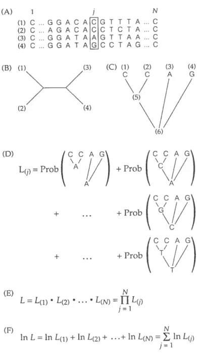
Once a substitution moclel is defined, the likelihood of a given tree is calculated to examine its consistency with the data. Figure 2.1 shows the main steps of calculating the likelihood of a tree.
In Figure 2.1(A), sequences of four taxa with length N are aligned together and vie want to calculate the probability of this alignment. Figure 2.1(3) is an example of one of the possible unrooted trees for these 4 taxa. As discussed earlier in this chapter, for the time-reversible models the position of the hypothetical root does not change the likelihood of the tree. Figure 2.1(C) shows an example of a rooted tree that is obtained by piacing the root at an arbitrary position. It is a.ssumed that the bases of a sequence evolve independently of each other. Hence, the likelihood of each column can be calculated separately and the likelihood of the tree is the product of the likelihoods for each column in the alignment (Fig. 2.1(E)).
In order to calculate the likelihood of colurnn
j,
ail possible scenarios that could generate the columnj
should be considered. Each of the hypothetical roots cari be an A, a C, a G or a T. Since there are 2 hypothetical roots with 4 possibilities for cadi, there are 4 x 4 = 16 different scenarios that could result in the colurnnj.
Given that cadi of these 16 cases are possible, then the total probability of tic columnj
is tic sum of these probabilities (Fig. 2.1(D)).Tic probability of alignment of n sequences wuich are related to eaci other by a phylogenetic tree, T, is equal to the likeliiood of tic tree and can be written as
L(T) = Pr(XT) =
Pr(XT)
where X is the alignment of length N (Durbin et al. 1998). The probability of each site under a given phylogenetic tree is Pr(XT) = Pr(., XT). In tus equation, is the state (i.e. A, C, G or T) of tie n — 1 hypotietical ancestral
nodes of tic tree.
(A) I (1) C G G A C 2) C A G A C (3) C G G A f (4) C G G A T (D) L(1) = Prob (3) (C) (1) (2) (5) (4) (6) CCA +Prob
(
\cÇ/
N = , in Lf/) i=1 ACGT ACC T AAGT AGCC N TTA..C CTA.,C TAA...C TAG...C (B) (1) (2) (3) (4)/
G))
+ CC + Prob (\G// + Prob T + (E) N L = L(fl• L(2) •L(N =U
L(f) j1 (f) In L =in L(1) +in L(2)+ .+ In L(N)Figure 2.1: Overview of calculating the iikelihood of a given phylogenetic tree (from Hiliis et al. 1996)
24 this likelihood (Durbin et al. 1998). A short surnmary of this rnethod is described next.
Suppose n is a node in T. If n is not a leaf, then let u, ‘w be the chuidren of node n. Suppose t anci t are brandi lengths t.hat connect y and w to their parent. If
we are given a model of evolution with its substitution probahility matrix P(t), tien we can calculate the probability that base a changes to base b in tirne t. Tus probability is equal to Pab(t). If u is a leaf, Pr(Lja,T) represents the probability of having base a at node n. If n is not a leaf, Pr(La, T) is the probability of ail the children of n when node n lias base a. This probability is calculateci from the probabilities Pr(Lb) and Pr(Lc) for ail possible values of b and e. Tic recursions are given as:
I(a r) if n is a leaf
Pr(L,11a. T) (ZbPub(tv) Pr(Lb. T)) . (2.4)
otherwise
X
(Z
Pac(tw) Pr(Lc, T))a,. is tic base of X at node n. I is the indicator function. The probability of cadi column of alignment, X, is defined hy Pr(XT) = na Pr(L7.ja, T), where r is tic hypothetical ancestor of ail sequences. This recursive procedure, implemented as a dynamic programming algorithm was introduceci by Felsenstein (1981). Using tus recursion, likeliiood of a single tree witi n leaves of length N anci alphabet of size m, can be calculated in O(nNm) tirne.
The maximum likeliliood estimate of a phylogeny tree can be expressed as:
= arg max Pr(XT) (2.5)
T
can be obtained by calculating the Pr(XT) for ail the possible tree topologies. Finding the optimum tree is a NP-harcl problem (Roci 2006; Chor and Tulier 2005). Therefore, for large number of taxa, heuristic searci techniciues are employed to obtain the near-optimal trees in reasonable computing time (Guindon and Gascuel 2003).
For three sequences, iikelihood of colurnn i of the alignment can be calculated as:
Pr(XT) = aPax(ti)Pax(t2)Pax(t3) (2.6)
a{A,C,G,T}
where is the base of jth sequence at colurnn i; and t is number of mutations occurred along the branch connecting jth sequence to the common ancestor of ail three.
2.3.1 Estimation of Model Parameters
From the above description, it eau be seen that several pararneters must be estimated from the data using maximum likelihood rnethod.
Q,
an instantaneous substitution rate matrix; •T, the tree topology; t, the vector of branch lengths and equilibrium base frequencies are those that are estimated.In some simple cases (three or four taxa), the optimum can be found analyti cally, but in most cases heuristic optimization is necessary. Different optimization methods can be used to estimate the parameters of a given tree. There are two major families of algorithms for optimization (Press et al. 2002). The first family are gradient-based approaches which use the objective function and its derivatives to estimate the optimal values of each parameter. For instance, Newton’s method, needs the first and second partial derivatives of the objective function with respect to each parameter (Hillis et al. 1996).
The second category, derivative-free optimization methods, do not need the derivative of the function and therefore are more practical. Brent’s method (1973), for a single variable; and Poweil’s method (1964), for several variables; are examples of this category (Press et al. 2002).
Ideally, the best tree should be found, by searching over the n dimensional pa rameter space, and giobally optimal values of these parameters should be reported at the end. This means that for every possible tree, all parameters should be op timized for that tree. The tree with the highest likelihood is selected as the best model (Hiffis et al. 1996).
26 2.4 Evolutionary Models with Gaps
Alignment of rnost seciuences contains gaps. Mutationai changes like insertions, deletions, and rearrangernent of genetic materials produce gaps in the alignrnent. Varions methods are irnplernented in pliylogenetic programs to t.reat the gaps, and each methoci lias its advantages and disadvantages. Cornrnonly, phylogenetic analysis programs ignore the colurnns of alignrnent that contain gaps (Siepel and Haussier 2004). This approacli lias the drawback tliat the alignrnent of divergent sequences may have only a small rninority of colurnns without any gaps.
McGuire et al. (2001) suggested to treat the gap as an extra character in the evolutionary model. Using this approach, a multiple-site insertion or deletion is considereci as a series of independent events. However, it is well known that gaps tend to lie persistent and to occur as a consecutive group ratlier tlian to be scattered individually (Durbin et al. 1998). Tlierefore, this approaci overweights multiple-site gaps when it cornes to calculating the likelihood of a tree (McGuire et al. 2001).
Boffeffi et al. (2003) replace the gaps in each colurnn with the least frecuent1y occurred hase in that column. Global eciuilibriurn base frequencies are used to break the ties. Since this thesis deals with three sequences, this approach is not appropriate.
In our program, two different approaches of treating gaps are implemented. Gaps can be treated either as missing data or they can be used to learn about their patterns through a tree-hidden Markov model (tree-HIVIM) architecture.
In the following sections, first I describe how gap can be treated a.s missing data. Next, the model proposed by Mitchison and Durbin (1995) is presented. This model, called tree-HMIVI, allows affine-type gap penalties to lie learned and incorporated into the standard evolutionary models.
2.4.1 Phylogeny and Missing Data
Many phylogeny programs, inciuding PHYLIF (Felsenstein 1993), treat gaps as missing data. In order to describe the method more precisely, the notation given by Siepel and Haussier (2004) is followed.
Suppose an alignment X is given. X is one of the columns of alignment with gaps. If gaps are replaced with a character from alphabet Z {A, C, G, T}, set M is obtained. Since every element of M could lead to have the colurnn X, the probability of X.j is obtained by summing over ail elements of M.
Pr(XT) Pr(yT)
yCM
The eiernents of X that are gaps can be seen as wildcards. For instance, by de noting * to gaps, X = (A, C, G, *,A)T wouid lead to
M = {(A, C, G, A, A)T, (A, C, G, C, A)T, (A C, G, G, A)T, (A, C, G, T, A)T}. Felsen stein’s formulas (E.q. 2.4) are extended to treat gaps as missing data (Felsenstein 2004). Equation 2.4 is generaiized to
I(a matches x) if u is a leaf
Pr(Lja,T) = (bPab(tv)Pr(Lvb,T)) (2.7)
otherwise
X
(
Pac(tw) Pr(Lc, T))Thus, if node u has a “t”,
Pr(La) = 1 for every possible a. This can be seen as removing the branch connecting u to its parent (IVlcGuire et al. 2001). Therefore, the gaps in the ahgnment neither remove nor add any information in inferring phylogenies. This approach has no additionai cost in calcuiating the likelihood of the tree. Throughout this thesis, this model is referred to as standard phylogeny mo del.
In this model, eaci coiumn of aiignment is independent of other columns. This means that if the columns of aiignment are shuffled, the likelihood of the resulted alignment is the same as the original alignment. Patterns of insertions and deletions
28 are not used in this model. Therefore, shared patterns of insertions and deletions which may disclose useful information about the relationship between secinences are ignored and are not taken into account (McGuire et al. 2001).
2.4.2 Tree-Hidden Markov Model
Tree-HMM takes into account the pattern of gaps in the alignment. This model is considered as the composition of an alignment model (i.e. a profile-HIVIIVI, Krogh et al. 1994) and a standard evolutionary model (Neyman 1971; Felsenstein 1981). In this model, alignment is regarded as a series of paths through an HMM-profile. Rearranging the columns of alignment would resuit in an aligilment with different likelihood from the origillal alignment.
Tree-HMM lias match (lvi) and delete (D) states. Insertions are not rnodeled with an explicit state; they happen wlien a sequence goes to a match state at a position whule its ancestor goes to a delete state.
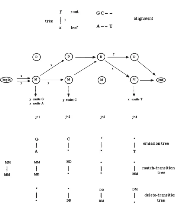
In order to describe the tree-HMM , we follow the description given by IViitchison
(1999). A simple phylogenetic tree, T, is sliown in Figure 2.2. This tree lias a sequence y at the root and sequence r at the leaf. This tree indicates tliat sequence r lias evolved from sequence y over time t. At cadi column of the aligument, each sequence lias an emission and a transition; these two are referreci to as the path of the sequence at that position. Figure 2.2 shows an example of tic paths r and y take at four columiis of tic aligument. The differences in tic paths eau lie either because they emit different nucleotides or they use different states and transitions. A probability is given to eaci pati at every column; multiplying ah these probabilities gives Pr(ay,T). The probability of having sucli an alignment is Pr(x, yt, T) = Pr(yT) Pr(ry, T), where Pr(yT) is tic prior probability of the root sequence.
At position 1, both sequences are in tie Match (M) state; x emits A while y emits G. Tus cari lie seen as a tree witi G at tic root and A at the leaf anci Pr(AG, t, T) = PGA(t) is computed from the substitution probability matrix of tic piylogeny model (Eq. 2.1).
Y root —
tree aligrnnent
X leaf A——T
rO
yemitsG yemitsC x emlisT
emitsA j=1 j=2 j=3 j=4 G C * *
I
I
I
emissiontree A * T MJT MJI *I
I
I
I
match-transition tree * DD DMI
I
I
I
DD DM treeFigure 2.2: A short tree-HMM for a simple tree with two nodes (from IViitchison 1999)
30
The tree that depicts the substitution of nucleotides is called the emission
tree in a tree-HMM. The probability of the column 1 in the emission tree is
Pr(A,
Git,
T) = 7IPr(AIG, t, T) where ir is the base frequency of nucleotide G.In going from position 1 to position 2, x has a transition from M state to D
state, whereas y bas a transition from M to M state. “MD” is useci for the former transition and “MM” for the latter. This substitution of transitions is denoted by Pr(IvIDMM, t, T). There are four possible substitutions of transitions from the match state and they form a 2 x 2 matrix:
(
Pr(MMIMM,t) Pr(MDIMM,t)(28)
Pr(MMMD,t) Pr(MDjMD,t)
)
which is called the match-transition family matrix, The substitutions of tran
sitions from match state define t.he match-transition Lree. This tree bas MM
at the foot and MD at the leaf at position 1. Pr(A1D, MMt., T) is equal to
rrp./IM Pr(MDMM, t, T). The prior probability of MM transition is denoteci by
1rMM.
At position 3, x has a DD transition and y a DM transition. The probability of this substitution of transition is denoted by Pr(DD, DMt, T) anci is equal to
DM Pr(DDDM, t, T). The delete-transition matrix is defined as:
(
Pr(DDDD,t) Pr(DMIDD,t)9
Pr(DDDM,t) Pr(DMDM,t)
)
The substitutions of transitions from delete state define the dcl etc-transition tree.
In positions Ï and 3 both sequences are in the same state, but they are in different
states in position 2 and 4; therefore, x can not be seen as being evolved from y
(Mitchison 1999). Mitchison and Durbin (1995) proposed that at these positions
the transitions of x and y should be regardeci independent of each other. The
symbol *
is used to denote the missing ancestor or descendant sequences at such
For example at position 2, delete-transition tree lias * at the root and DD at
the leaf.
Pr(DD, *t, T) 7rDjI Pr(DDIDM, t, T) + 7CDD Pr(DMDD, t, T)
DD (Pr(DDDD, t, T) + Pr(DMDD, t, T))
=
The second step in the above calculation is based on the assumptioi that t.he delete-transition matrix is reversible. In the similar manner, at position 2, MD is at the root of match-transition tree and * is at the leaf, therefore
Pr(*, MDt, T) = 7rjr Pr(MMMD, t, T) + 7CAID Pr(MDMD, t, T)
= MD
At the positions of the tree where ancestor and descendant at both root and leaf are missing, Pr(*, *T) = Ï.
Pr(x, yT) is calculated by multiplying the prohahilities of ail transitions and
emissions of x and y. Suppose E(r) denotes the emission of at position i. At
position i, r can be either in match state or deiete state. Let M(x) 5e the transition
from the match state or *
if x does not use match state at position i. Suppose
D(x) denotes the transition from the delete state by sequence x at position i or *
if delete state is not used. Then the joint probability of alignment of x and y can
5e expressed as:
N
Pr(x, yT, t)
=
fl
Pr(M(x), ‘i(y)) x Pr(D(), D(y))x Pr(E(x), E(y))
32 and
Fr(xIT)
is calculated by snrnming over ail possible paths of the root sequence:Pr(xIT)
=fl
Pr(M(x) T) Pr(D(x) T) Pr(E’(x) T)Pr(E(x)T),
the
probabihty of the emission of r at position i, is calculated hy summing over ail possible root residues. Pr(IVI(x)T) is obtained by summing overail possible match transitions of the root. Similarly, Pr(D(x)T) is defined by summing over ail possible delete transitions of the root.
The probability of a tree T with n leaves modeled by a tree-HIVI]\/1 is:
Pr(i,. , T)
fl fl
Pr(S(i),... , $(xT) (2.10) i=1 Swhere $ is E, M or D; and N is the number of columns in the alignment (Mitchi son 1999). This probability can be calculated using the dynamic programming algorithm of Felsenstein. The above probability can be regarded as:
Pr(r1 = L(emission tree) x L(match-transition tree)
x L(delete-transition tree) (2.11)
where L is the likelihood. Since the columns of alignment are assurned to be indepenclent of each other, likelihood of each tree is the product of the likelihoods for every column of alignment for that tree.
IViitchison used the following form for the match-transition matrix
(Ï_a)(1_e_Tt)
(2.12)
a — ae_Tt 1
— a + ae_rt
)
The rows and columns of this matrix correspond to the MM and MD transitions respectively. In this matrix, t represents the time elapsed since sequence x divergeci from its ancestor; r O is a rate constant; and O < a < 1 is the equilibrium
probability of “IVIM” transition. The equilibrium frequencies are used as the priors: = a and 7rfD = 1—a. TRis form of matrix is time reversible and multiplicative (I\’Iitchison 1999). Delete-transition matrix is also assumed to have the same forrn but with different parameters.
(b + (1 — b)e (1 — b)(1 — (2.13) b — be’t 1 — b + be_ut
J
The rows and columns correspond te DD and DM respectively. Similarly nDD = b
and ‘JrD,J 1 — b and u O is a rate constant.
As previously mentioned, in tRis thesis we are working with three sequences. Likelihood of colurnn i in a tree-HMM for three sequences is calculated as:
Pr(XT)
=
(
n (Pr(E(xi)v, t,) Pr(E’(x2)v, t2) Pr(E3)v, t3)) \vE{A,C,G,T} x n (pr(Mz(xi)m. t,) Pr(Mz(x2)rn,t2) Pr(M’(:3)Im,,t:3)) \rnE{MM.AÏD} x n \oE {DD ,DM} (2.14)where [t,,t2,t3] is the divergence time vector. In Equation 2.14, Pr(Ez(xj)v,tj) is calculated from the substitution probability matrix P(t) (Eq. 2.3); Pr(M(xm, t) is calculated from the match-transition family matrix (Eq. 2.12); and Pr(Dz(xj)o, t) from delete-transition family matrix (Eq. 2.13).
2.5 Phylogenetic Analysis Tools
Several phylogenetic analysis programs are available. The main ones are PHYLIP, phylogenetic inference package (Felsenstein 1989-1996); at
34
phvlogenetic analysis using parsimony; at http //www. ims si edu/PAUP/.
The three main methods of phylogenetic analysis (parsimony-based. distance-based and maximum likelihood) are implemented inthese two packages. A comprehensive list of available packages and servers are listed at http: //evo lut ion. genetics. washington. edu/pliylip/software.html.
There are also a few useful Web sites that. provide information on phylogenetic relationships among species and organisms. Among them, tree of life at http: // tolweb.org/tree/ and Taxonomy buowser at http://pubmedexpress.nih.gov/ Taxonomy/ can be rnentioned.
METHODOLOGY
The assumption about equaÏ rate of evolution along a sequence is often unrealis tic (felsenstein and Churchill 1996). I\’Iutational and selective pressures vary with nticieotide position in a genorne (Nielsen 2005). The evolutionary forces affecting
a nucleotide in a genomic sequence depend on miscelianeous factors, including lo
cal sequence context, and whether the nucleoticle belongs to coding or non-cocling region. The model of sequence evolution that imposes the same rate of evolution across ail columns of a multiple alignment is used as nuit hypothesis in this the
sis. Felsenstein (1981) and Neyman (1971) used this nuil hypothesis in maximum
likelihood methods to infer phylogenies (Felsenstein and Churchill 1996).
Heterogeneous evolutionary rates at different sites in molecular sequences are addressecl by different authors, including Yang (1993, 1994); Kelly anci Rice (1996); Felsenstein and Churchill (1996).
We have employed heterogeneous evolutionary rates to reach our objective which is to find the signatures of negatively and positively selected regions in closely relatecl genomes. Here, we limit the number of sequences under stuclv to
three. However, our methoci can he readily adapted to more than three secluences. The sequences under study can be aligned using any publicly available multiple alignment tool. The alignrnent of these sequences is used as the input of our pro-gram.
Three rate categories are defined: neutral, slow and fast. Neutral rate regions represent the positions in a genorne that have accumulated mutations over time and
have not been under selection. These regions are assumed to be non-functional. Slow rate regions represent the positions in a genome that have been uncler negative selection and have tmdergone little changes since the separation from the species’ rnost recent common ancestor. These regions are likely to be functional.