HAL Id: hal-01716280
https://hal.archives-ouvertes.fr/hal-01716280
Submitted on 15 Feb 2019
HAL is a multi-disciplinary open access
archive for the deposit and dissemination of
sci-entific research documents, whether they are
pub-lished or not. The documents may come from
teaching and research institutions in France or
abroad, or from public or private research centers.
L’archive ouverte pluridisciplinaire HAL, est
destinée au dépôt et à la diffusion de documents
scientifiques de niveau recherche, publiés ou non,
émanant des établissements d’enseignement et de
recherche français ou étrangers, des laboratoires
publics ou privés.
Design and optimization of three-dimensional extrusion
dies, using constraint optimization algorithm
Nadhir Lebaal, Fabrice Schmidt, Stephan Puissant
To cite this version:
Nadhir Lebaal, Fabrice Schmidt, Stephan Puissant. Design and optimization of three-dimensional
extrusion dies, using constraint optimization algorithm. Finite Elements in Analysis and Design,
Elsevier, 2009, 45 (5), pp.333-340. �10.1016/j.finel.2008.10.008�. �hal-01716280�
Design and optimization of three-dimensional extrusion dies, using constraint
optimization algorithm
Nadhir Lebaal
a,∗, Fabrice Schmidt
b, Stephan Puissant
aaGIP-InSIC, ERMeP, Institut Supérieur d'Ingénierie de la Conception, 27 Rue d'Hellieule, 88100 Saint-Dié, France bEcole des mines d'Albi Carmaux, Laboratoire CROMeP, Campus Jarlard- Route de Teillet, 81013 Albi Cedex 9, France
A B S T R A C T
Keywords: Polymer extrusion Response surface method DoE
Optimization Kriging interpolation Finite element analysis
Balancing the distribution of flow through a die to achieve a uniform velocity distribution is the primary objective and one of the most difficult tasks of extrusion die design. If the manifold in a Coat-hanger die is not properly designed, the exit velocity distribution may be not uniform; this can affect the thickness across the width of the die. Yet, no procedure is known to optimize the coat hanger die with respect to an even velocity profile at the exit. While optimizing the exit velocity distribution, the constraint optimization algorithm used in this work enforced a limit on the maximum allowable pressure drop in the die; according to this constraint we can control the pressure in the die. The computational approach incorporates three-dimensional finite element simulations software Rem3D!and includes an optimiza-tion algorithm based on the global response surfaces with the Kriging interpolaoptimiza-tion and SQP algorithm within an adaptive strategy of the search space to allow the location of the global optimum with a fast convergence. The optimization results which represent the best die design are presented according to the imposed constraint on the pressure.
1. Introduction
The design of dies for polymer extrusion often involves trial and error corrections of the die geometry to achieve uniform flow at the exit. If the repartition channel in a flat die is not designed properly, the velocity at the exit of the flat die may not be uniform[1], and leads to a variation in the sheet thickness across the width of the die. Often, the number of the involved variables and their interactions prevent any optimization according to the trial and error corrections, because the number of evaluations needed may become very high. Design of experiment, in particular the Taguchi method[2], allows obtaining invaluable information on the important variables of the process in order to achieve the required goals. The effects of the var-ious factors can be represented on graphs to support the discussion and to lead to identify the most sensitive to minimize the defects. Within this framework, we can mention Chen et al.[3]. They showed, using the Taguchi method, that the operating conditions, the type of materials, and the geometry of the die have a great influence on the exit velocity distribution on the die.
Prior works in sheet die optimization have involved the use of lubrication approximations of the momentum equations[4,5]. If the
∗ Corresponding author. Tel.: +33 329 421 821; fax: +33 329 421 825. E-mail addresses:[email protected],[email protected](N. Lebaal).
geometry is more complex, a flow channel can be approximated with simple geometric sections[6]. Smith et al.[7,8]modeled Newtonian and non-Newtonian isothermal flow in a coat hanger die using a generalized Hele–Shaw (HS) approximation, and optimized the die by minimizing pressure drop subject to exit flow uniformity being within a tolerance set. The sensitivities analysis needed for the se-quential quadratic programming (SQP) algorithm was calculated by direct differentiation and the adjoint method are compared, and si-multaneous minimization of velocity dispersion subject to residence time variations is added using Broyden Fletcher Goldfarb Shanno (BFGS) algorithm and penalty function. The same author[9]in order to optimize the shape of the extrusion die for two different mate-rials at various temperatures, used and compared two optimization algorithms with constraint based on SQP and sequential linear pro-gramming (SLP). The optimization problem consists in minimizing the pressure loss in the die, with an imposed constraint so that a homogeneous velocity distribution is obtained on the outlet side of the die within an imposed tolerance. Network algorithms have been developed to optimize die designs[10]but they are difficult to ap-ply to arbitrary shapes. Michaeli et al.[11]have used a combination of finite element analysis for isothermal flow and flow analysis net-work to accelerate the iterative optimization process for the design of profile extrusion dies. To optimize the die geometry, they used, respectively, the evolution strategy algorithm and network theory. Sun et al.[12]optimize a flat die using BFGS algorithm. A penalty
Nomenclature
a, m,
!
, A1, A2 material constantsˆa
"
coefficients vectors#
weight coefficientA, B, C, D optimization variables
c dilation parameter
di distance from a discrete node xito
a sampling point x
E velocity dispersion
E0 initial velocity dispersion
$
(v) strain rate tensor !$
toleranceF(x) responses from the function
g constraint function ˙¯
%
shear rate&
fluid viscosity (dependent of thetemperature T, pressure p, and of the strain rate tensor
$
(v) through the shear rate ˙¯%
)&
0(T) thermal dependencyJ normalized objective function !J(x) objective or constraint interpolate
function
k number of the basis function in re-gression model
N number of nodes at the die exit
P pressure
P0 initial pressure in the die
ˆp(x) basis function
R correlation matrix
rw radius of support domain
S1, S2, S3 surfaces
T temperature
Tref references temperature
v velocity
vi exit velocity
v average exit velocity
wi(x) weight function of Gaussian type
x design variables
Z(x) random fluctuation
function was introduced to enforce a limit on the maximum allow-able pressure drop in the die.
The optimization algorithm must be carefully chosen when one single analysis using three-dimensional software requires several hours of CPU time. Non-deterministic or stochastic methods such as Monte Carlo method and genetic algorithm[13] can obtain global minimum but they need a lot of evaluations for the functions to converge. Gradient methods[7–10,12,14]require the computations of the gradients of the functions; the computation of gradients by finite difference is time consuming and depends on the perturbed parameters. For the above reasons we decided to chose a response surface method (RSM)[15].
The ultimate goal of this work is to optimize the coat hanger sheet die geometry (Fig. 1) in a way that a uniform velocity distribution is obtained at the die exit with an imposed nonlinear constraint so that the pressure loss in the die must decrease compared to the initial die. For this end, we developed an automatic optimization algorithm based on SQP algorithm and a RSM together with Kriging interpo-lation and several strategies to permit to obtain a precise global optimum with a fast convergence. A preliminary study based on Taguchi's design of experiments method[3]was conducted, in or-der to identify the most sensitive design variables. To compute a 3D flow in extrusion dies we used FEM software (REM3D
!
)[16]. This software takes into account strain rate and temperature dependence.2. Modeling and simulation
The extrusion simulation is carried out using the 3D computation software by finite elements REM3D
!
[16].The flow equations are derived from the Navier–Stokes incom-pressible equations. A mixed finite element method for incompress-ible viscous flow is used. The flow solver uses tetrahedral elements with a linear continuous interpolation of both the pressure and the velocity and a bubble enrichment of velocity.
The mass, momentum and energy conservation equations, are used to follow the material behavior, from which the velocity, pres-sure and temperature fields are determined.
⎧ ⎪ ⎪ ⎨ ⎪ ⎪ ⎩ ∇(2
&
(˙¯%
)˙$
(v)) − ∇p = 0 ∇ · ⃗v = 0'
ˆcdTdt = −∇ ·q +(
: ˙$
(v) (1)The behaviors laws used in Rem3D
!
give an expression of the viscosity in function of the shear rate and temperature. In this paper, the geometry of a flat die is optimized for an acrylonitrile butadiene styrene (ABS, Astalac EPC 10000). The rheological parameters of the ABS are given inTable 1. Carreau Yasuda/WLF viscosity model is used to characterize the temperature and shear rate dependence[17]. It is written as&
=&
0(T) & 1 + '&
0(T)!
%
˙¯ s (#)m−1/# (2) In this model, a, m,!
are material constants, whereas&
0(T)estab-lishes the thermal dependency, given by the WLF model:
&
0(T) =&
0(Tref) exp& A1(Tref− Ts) A2+ (Tref− Ts) − A1(T − Ts) A2+ (T − Ts) ) (3) where A1, A2are material constants, and Trefis the references
tem-perature.
A flow of 50 000 mm3/s was imposed on the entry with a
tem-perature of 240◦C, and the temperature of the die is constant and
equals to 230◦C.
3. Formulation of the optimization problem
3.1. Objective and constraint functions
This optimization problem consists in determining an optimal ge-ometry to homogenize the velocity distribution through the die exit, which corresponds to the minimum of the velocity dispersion (E). While preventing that the pressure “pressure loss” increases more than the pressure obtained by the initial geometry. We can also impose a more severe constraint on the pressure; this condition is translated by a constraint function (g).
⎧ ⎪ ⎪ ⎨ ⎪ ⎪ ⎩ min J(
)
) =EE 0 such that g =P − (#(#
∗ P∗ P0) 0)!
0 (4)where (J), the normalized objective function, the velocity dispersion (E), is defined as E = ⎛ ⎝1 N N , i=1 -|vi− v| ¯v .⎞ ⎠ (5)
Variable A Variable D Variable B Variable C y mm x mm h = 4 h = 2.67 h = 6.7 z mm 50 36.5 25 25 112.6 156.5161.5 206.5 221.5 45 426.3
Fig. 1. Geometry of the flat die. Table 1
Rheological parameters
&0(Pa s) m #0 !s(Pa)
716.997 0.15862 1 224063
A1 A2(K) Ts(K) Tref(K)
20.4 101.6 397.7 524.7
where E0 and P0 are, respectively, the velocity dispersion and the
pressure in the initial die, N is the total number of nodes at the die exit in the middle plane, viis the velocity at an exit node, and v is
the average exit velocity, is defined as
v =N1
N
,
i=1
vi (6)
The constraint function (g) is selected in a way that it is negative if the pressure is lower than the imposed pressure, if not it will be positive. If
#
= 1; the pressure should not increase compared to the initial pressure. If#
<1; the pressure must be even lower compared to the initial pressure.3.2. Design variables
The design of a flat die is based on the values of various geometri-cal parameters; the optimization variables (A, B, C and D) correspond to the geometry of the coat hanger die. The first variable A represents the depth of the channel repartition, the second variable B represents the opening of the channel repartition, the third one C represents the channel thickness and the fourth variable D represents the thickness of the relaxation zone (Fig. 1). During the optimization process the variables A, B, C and D vary in a limited field. Each variable has its geometrical limitations which are, respectively, 30
!
A!
110 mm, 50!
B!
140 mm, 5!
C!
45 mm and 6.7!
D!
15 mm.Initially, the four geometrical variables of the die are A = 36.5 mm,
B = 112.6 mm, C = 25 mm and D = 6.7 mm.
Surface (S1)
Surface (S2)
Surface (S3) Ni (xi yi zi)
Fig. 2. Procedure for the change of the geometry.
During the optimization process, we developed a Matlab
!
-based program which, allows us to treat the CAD and to change the geom-etry of the die automatically. In the first stage, in order to change the geometry we make a surfaced mesh. Since we know the nodes position, we seek to determine the coordinates of all the nodes (Ni),belonging to both surfaces S1, S2 and S3 (Fig. 2). For this, we use the diffuse approximation[14]with a linear interpolation.
To change the geometry of the channel repartition we define the new surface (S1k), which corresponds to the new optimization
pa-rameters Ak, Bk, and Ck. After that, we carry out a change of
coordi-nates for all nodes which belong to the surface S1, so that they will be relocated on to the new S1ksurface which represents the new
ge-ometry. For S2 and S3 surface, a simple translation of the following nodes is applied there. The same procedure is applied on the other side of the die.
3.3. Optimization procedure
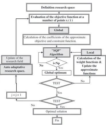
The objective and constraint function (Eq. (4)) are implicit pared to the optimization parameters and its evaluation need a com-plete numerical analysis of the extrusion process, which requires a large computation times. To need the optimum parameters with low cost and with a good accuracy, the RSM is adopted and cou-pled with an auto adaptive strategy of the research spaceFig. 3. The RSM consists in the construction of an approximate expression of objective and constraint function starting from a limited num-ber of evaluations of the real function. In order to obtain a good
Evaluation of the objective function at a number of points x ( i ) Definition research space
No "SQP"
Algorithm
Calculation of the coefficients of the approximate objective and constraint function.
TEST
Calculation of the weight functions &
Update the approximate functions Global optimum i<Np No Yes Local Global Yes Yes Update of the research field TEST No Optimal solution j = j + 1 Fin Auto adaptative research space.
Fig. 3. The flowchart of the adopted optimization strategy.
approximation, we used a Kriging interpolation described in next section. In this method, the approximation is computed by using the evaluation points by composite design of experiments.
Once the approximation of the objective function and the con-straint function are built for each iteration. Since the successive eval-uation of the approximate function does not take much computing time, we use the SQP algorithm to obtain the optimal approximate solution which respects the imposed nonlinear constraints. To avoid the fact of falling into a local optimum, and to respect the imposed nonlinear constraint, we use an automatic procedure which allows the launch of the SQP algorithm starting from each point of our ex-perimental design (Fig. 3). We take then the best approximate so-lution among those obtained by the various optimizations. Then, another approximate function is built by taking into account the weight function of Gaussian type which allows to slightly change the interpolation and makes the approximation more accurate locally (centred around the best minimum). Next, another minimization is carried out by the SQP algorithm with the initial point which rep-resents the best optimum The iterative procedure stops when the successive points of the approximate function are superposed with a tolerance !
$
= 10−6. Finally, another evaluation is carried out toob-tain the real response in the optimization iteration.
An adaptive strategy of the search space is applied to allow the location of the global optimum and, then, to readjust the research space by decreasing it by1
3. A new design of experiment is
automati-cally launched around the optimum. An enrichment of the interpola-tion is made by recovering responses already calculated, and which are located in the new research space. The iterative procedure stops when the successive points are superposed with a tolerance!
$
=10−3.3.4. Kriging interpolation
The Kriging interpolation[18,19], makes it possible to present the complexes function effectively. This method is applied in our work to represent the response surface in an explicit form, according to
the variables of optimization. The approximate explicit relationship of the objective and constraint function, can be expressed as follows: !J(x) = ˆpT(x)ˆa + Z(x) (7)
with ˆp(x) = [ˆp1(x), ... , ˆpk(x)]T, where k denotes the number of the
basis function in regression model, ˆa = [ˆa1, ... , ˆak]Tis the coefficient
vector the, x is the design variables,!J(x) is the unknown objective or constraint interpolate function, and Z(x) is the random fluctuation. The term ˆpT(x)ˆa in Eq. (7) indicates a global model of the design space,
which is similar to the polynomial model in a moving least squares (MLS) approximation. The second part in Eq. (7) is a correction of the global model. It is used to model the deviation from ˆpT(x)a so
that the whole model interpolates response data from the function The construction of a Kriging model can be explained as follows: The output responses from the function are given as
F(x) = {f1(x), f2(x), ... fn(x)} (8)
From these outputs the unknown parameters ˆa can be estimated: ˆa = (ˆPTR−1ˆP)−1ˆPTR−1F (9)
where ˆP is a vector including the value of ˆp(x) evaluated at each of the design variables and R is the correlation matrix, which is composed of the correlation function evaluated at each possible combination of the points of design:
R = ⎡ ⎢ ⎣ R(x1, x1) · · · R(x1, xn) .. . ... ... R(xn, x1) · · · R(xn, xn) ⎤ ⎥ ⎦ + ⎡ ⎢ ⎢ ⎢ ⎣ w(x − x1) 0 · · · 0 0 w(x − x2) · · · 0 .. . ... ... ... 0 0 · · · w(x − xn) ⎤ ⎥ ⎥ ⎥ ⎦ (10) Rij= (|xi− xj|) (11)
A weight function of Gaussian type with a circular support is adopted for the Kriging interpolation. It takes the form
wi(x) = ⎧ ⎪ ⎨ ⎪ ⎩ ' 1 −e−(di/c) 2 − e−(rw/c)2 1 − e−(rw/c)2 ( si di
!
rw 1 si di"
rw (12)where di=78nJ=1(xJ− xJ(i))2is the distance from a discrete node xi
to a sampling point x in the domain of support with radius rw, and
cis the dilation parameter. c = rw/4 is used in computation.
The second part in Eq. (7) is in fact an interpolation of the residuals of the regression model ˆpT(x)ˆa. Thus, all response data will be exactly
predicted; is given as
Z(x) = rT(x)
"
(13)where rT(x) = {R(x, x1), ... , R(x, xn)}.
The parameter
"
is defined as follows:"
= R−1(F − ˆPˆa) (14)4. Result and discussion
4.1. Design sensitivity analysis
A Taguchi's design of experiments method[3]is used to investi-gate the sensitive analysis of the design variables. This preliminary
0 20 40 60 80 100 1
Level of the variables of optimization
Ef
fect on the objective function
Variable A Variable B Variable C Variable C
2 1 2 1 2 1 2
Fig. 4. Effect of the variables on the objective function.
0 5 10 15 20 25 1
Level of the variables of optimization
Effect on the constraint function
Variable A Variable B Variable C Variable D
2 1 2 1 2 1 2
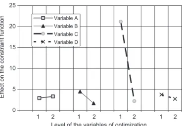
Fig. 5. Effect of the variables on the constraint function.
study was conducted, by considering four geometrical parameters (A, B, C and D), in order to identify the most sensitive ones on the objective and the constraint function.
For this, we have calculated the effect of each variable over all the field of research by studying the contribution of each variable on the variation of the response “velocities distribution and pressure”. The effects of the various variables are represented on graphs to support the discussion and to lead to the identification of those influencing to minimize the defects.
We note inFig. 4 that the variable with less influence on the objective function is the variable D which represents the thickness of the relaxation zone. On the other hand, the variable C has the greatest effect on the velocity distribution at the die exit.
We observe in the seam figure that if the variables “A, B, and
C” are in the lowest level (1), the global relative variation is more important which implies a bad velocity distribution at the die exit. On the other hand, if the variables are in the highest level (2), the global relative variation of velocity at the die exit is less important compared to their lowest level.
For the variable “C”, it is even weaker at the average level, and for the variable “D”, it is noted that it has a very weak effect over the velocity distribution at the die exit.
FromFig. 5we note that the effect of the variables B and D on the constraint function (pressure) is weak. We note that the more the variables “A, C and D” are in the lower level the more the pressure increases. On the other hand, the pressure is lower at their highest level. For the variable B, the variation of the pressure is very weak.
Fig. 6. Convergence history during an optimization process on the objective functions. Table 2
Summary of the results
Results of optimization Initial die (A) Result 1 Result 2 #= 0.5 (B) #= 0.35 (C) “J” 1 0.049 0.09 Improvement (%) − 95 91 “g” 1 0.48 0.38 Profit of pressure (%) – 52 62 Variable A (mm) 36.5 96.6 103.08 Variable B (mm) 112.6 76.15 72.74 Variable C (mm) 25 25.47 31.4
Since the prime objective in the design of the extrusion dies is to obtain at the exit a perfectly homogeneous product, it was noted that the variable D has the least important effect on the velocity distribution at the die exit. This study enables us to limit the number of variables and three sensitive geometrical parameters are selected and considered as design variables to be optimized (A, B and C).
4.2. Optimization results
The optimization strategy described previously is applied to op-timize the die geometry in order to obtain a homogenous exit ve-locities distribution. According to the imposed constraint on the pressure, two optimization cases are formulated:
Case1: A constraint on the pressure is imposed for which the pressure in the optimal die must be lower or equals 0.5∗P0(
#
= 0.5).Case2: The constraint imposed on the pressure is more severe. The pressure in the optimal geometry must be lower or equals 0.35∗P0(
#
= 0.35).A representative convergence history during an optimization pro-cess on the objective functions (J) is represented inFig. 6. After three iterations, the objective function fell below the cutoff of 10−3 and
the simulation stopped.
Given the fixed geometry constraints of the die, the rheological parameters of the ABS resin, and the process conditions, the optimal solution is obtained starting from the second iteration for both cases. The objective function is then reduced to 95% of its initial value for the first case (
#
= 0.5) and 91% for the second case (#
= 0.35). The optimization strategy clearly showed its capacity to obtain an optimal solution with a very fast convergence. A summary of the optimization results obtained for the two cases, is reported inTable 2.We notice that the objective function for both cases has strongly decreased in the first iteration, because of the precision of the Krig-ing interpolation. Nevertheless, to respect the constraint while en-suring a homogeneous distribution of velocity, we observe that case 1 offer the best minimum, because of the less severe constraint on the pressure compared to case 2.
We have represented the relative velocity dispersion obtained in the initial geometry and after optimization, for both results in
Fig. 7. We see that the objective function obtained by imposing a severe constraint on the pressure (
#
= 0.35) is slightly higher of the objective function obtained with a less severe constraint (#
= 0.5).Fig. 7. Velocity dispersion with initial and optimal die.
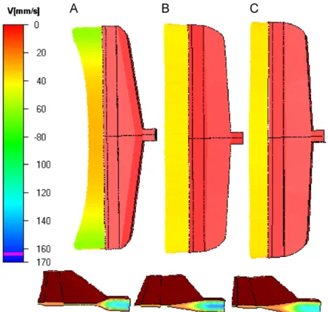
Fig. 8. Velocity distribution in initial and optimal dies.
For a qualitative comparison it is obvious that velocity distribu-tion in the initial geometry (Fig. 8A) is not homogeneous. We notice that in the middle of the die, velocities are lower about 35% of varia-tion compared to the average. On the other hand, in both parts close to the end of the die, we observe an increase of velocities until 50% (Fig. 7), only in the small regions near the end of this die, the exit velocity reduces to zero to satisfy the no slip condition at the walls. After optimization, we notice that velocities became homogeneous all over the width at the die exit. For both optimization results, see-ing, respectively,Fig. 8B and C.
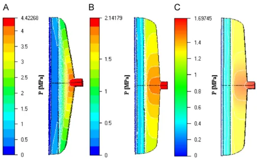
Fig. 10. Pressure distribution in initial and optimal dies.
Fig. 11. Temperature distribution in mid plane in initial and optimal dies.
The constraint on the pressure is represented onFig. 8, in a form of (P/P0) for both cases. We observe that the constraint function is
weaker with a more severe constraint (
#
= 0.35).This optimization problem was formulated in a way to find the best velocity distribution at the die exit while avoiding the increase of pressure compared to an imposed pressure, which is respected by both results (Fig. 9). The pressure drop in the design of the initial die is 4.42 MPa (Fig. 10A). It should be noted that the pressure decreases during the iterations of optimization for the different results. In the first case, the pressure decreases by 52% which gives a pressure of 2.14 MPa (Fig. 10B). In the results of the second case, we note that the pressure has decreased by 62% because of the imposed constraint (Fig. 9), which gives a pressure of 1.69 MPa (Fig. 10C). We notice that the gradient pressure in the initial die is not parallel, which results on a non-uniform flow. Nevertheless, in the optimized dies
the gradient pressure is parallel; furthermore, it denotes a uniform flow distribution for both cases.
It is noted that more the polymer runs towards the border because of the heating by shearing, the temperature is lower in the middle of the die and higher close to the border (Fig. 11A). By comparison, the distribution of the temperatures is uniform in the optimal die (Fig. 11B and C), because of the homogeneous velocities distribution (due to the heating by shearing) at the die exit for the optimal ge-ometries.
5. Conclusion
The design of polymer extrusion dies is complicated by the non-linear relationship between the resin viscosity, shear rate and tem-perature. The first study based on the sensitive analysis enabled us to decrease the number of variables by analyzing their effects on the pressure and the velocity distribution at the die exit. The numerical optimization algorithm presented in this work shows its robustness as a tool for extrusion die design. The applied optimization method with the various strategies proves its ability of predicting optimal die geometry with satisfactory computing time for three-dimensional finite element calculation.
The obtained results with the two optimization examples show that our optimization strategy is well adapted to the nonlinear con-straints. The use of the different constraints on the pressure allowed us to compare the various results obtained after optimization. The optimal die gives a good exit velocity distribution while minimizing the pressure for the same flow. A qualitative comparison enables us to note that we were able to obtain with the optimal geometry a 95% profit of homogeneity compared to the initial geometry with a decrease of pressure of 52% (results obtained with a less severe constraint on the pressure). The algorithm of optimization clearly showed its robustness and its capacity to obtain an optimal solution with a fast convergence.
Future research will involve experimental verification of the al-gorithm and the optimization of complex helicoidally dies.
References
[1] Y. Wang, The flow distribution of molten polymers in slit dies and coat hanger die through three-dimensional finite element analysis, Polym. Eng. Sci. 31 (1991) 204–212.
[2] D.C. Montgomery, Design and Analysis of Experiments, John Wiley & Sons, Inc, USA, 2005.
[3] C. Chen, P. Jen, F.S. Lai, Optimization of the coat hanger manifold via computer simulation and orthogonal array method, Polym. Eng. Sci. 37 (1997) 188–196.
[4] Y.W. Yu, T.J. Liu, A simple numerical approach for the optimal design of an extrusion die, J. Polym. Res. 5 (1998) 1–7.
[5] Y. Xiaorong, S. Changyu, L. Chuntai, W. Lixia, Optimal design for polymer sheeting dies, Chines J. Comput. Mech. 21 (2004) 253–256.
[6] S. Puissant, Y. Demay, B. Vergnes, Two-dimensional multilayer coextrusion flow in a flat coat-hanger die. Part I: modeling, Polym. Eng. Sci. 34 (1994) 201–208. [7] D.E. Smith, D.A. Tortorelliav, C.L. Tucker, Optimal design for polymer extrusion. Part I: sensitivity analysis for nonlinear steady-state systems, Comput. Methods Appl. Mech. Eng. (1998) 283–302.
[8] D.E. Smith, D.A. Tortorelliav, C.L. Tucker, Optimal design for polymer extrusion. Part II: sensitivity analysis for weakly-coupled nonlinear steady-state systems, Comput. Methods Appl. Mech. Eng. (1998) 303–323.
[9] D.E. Smith, An optimisation-based approach to compute sheeting die designs for multiple operating conditions, SPE ANTEC Technical Papers, 2003, pp. 315–319. [10] P. Hurez, P.A. Tanguy, D. Blouin, A new design procedure for profile die, Polym.
Eng. Sci. 36 (1996) 626–635.
[11] W. Michaeli, S. Kaul, T. Wolff, Computer aided optimisation of extrusion dies, J. Polym. Eng. 21 (2001) 225–237.
[12] Y. Sun, M. Gupta, Optimization of a flat die geometry, SPE ANTEC Technical Papers, 2004, pp. 3307–3311.
[13] W. Michaeli, S. Kaul, Approach of automatic extrusion die optimisation, J. Polym. Eng. 24 (2004) 123–136.
[14] H.J. Ettinger, J. Sienz, J.F.T. Pittman, A. Polynkin, Parameterization and optimisation strategies for the automated design of U PVC profile extrusion dies, Struct. Multidisc. Optim. 28 (2004) 180–194.
[15] N. Lebaal, S. Puissant, F.M. Schmidt, Rheological parameters identification using in-situ experimental data of a flat die extrusion, J. Mater. Process. Tech. Papers 34 (2005) 1524–1529.
[16] L. Silva, Viscoelastic compressible flow and applications in 3D injection molding simulation, Thèse de Doctorat, CEMEF, 2004.
[17] G. Balasubrahman, D. Kazmer, Thermal control of melt flow in cylindrical geometries, SPE ANTEC Technical Papers, 2003, pp. 387–391.
[18] I. Kaymaz, Application of Kriging method to structural reliability problems, Struct. Safety 27 (2005) 133–151.
[19] H. Li, Q.X. Wang, K.Y. Lam, Development of a novel meshless local Kriging (LoKriging) method for structural dynamic analysis, Comput. Methods Appl. Mech. Eng. 193 (2004) 2599–2619.