HAL Id: dumas-01267161
https://dumas.ccsd.cnrs.fr/dumas-01267161
Submitted on 4 Feb 2016
HAL is a multi-disciplinary open access
archive for the deposit and dissemination of sci-entific research documents, whether they are pub-lished or not. The documents may come from teaching and research institutions in France or abroad, or from public or private research centers.
L’archive ouverte pluridisciplinaire HAL, est destinée au dépôt et à la diffusion de documents scientifiques de niveau recherche, publiés ou non, émanant des établissements d’enseignement et de recherche français ou étrangers, des laboratoires publics ou privés.
communautés pélagiques de l’océan Atlantique tropical
et de l’océan Indien : comparaison de la pêche sous
dispositifs de concentrations de poissons et sur bancs
libres
Charlie Widehem
To cite this version:
Charlie Widehem. Impact de la pêche thonière à la senne sur les communautés pélagiques de l’océan Atlantique tropical et de l’océan Indien : comparaison de la pêche sous dispositifs de concentrations de poissons et sur bancs libres. Sciences du Vivant [q-bio]. 2015. �dumas-01267161�
Impacte de la pêche thonière à al senne sur
les communautés pélagiques de l’océan
Atlantique et de l’océan Indien : comparaison
de la pêche sous dispositifs de concentration
de poissons et de la pêche en bancs libres.
Par : Charlie WIDEHEM
Soutenu à Rennes le 11 Septembre 2015
Devant le jury composé de :
Président : Didier Gascuel
Maître de stage : Frédéric Ménard et Monique Simier Enseignant référent : Etienne Rivot
Autres membres du jury (Nom, Qualité)
Les analyses et les conclusions de ce travail d'étudiant n'engagent que la responsabilité de son auteur et non celle d’AGROCAMPUS OUEST
AGROCAMPUS OUEST CFR Angers CFR Rennes Année universitaire : 2014-2015 Spécialité : Halieutique
Spécialisation (et option éventuelle) : Ressource, Ecosystèmes Aquatiques
Mémoire de Fin d'Études
d’Ingénieur de l’Institut Supérieur des Sciences agronomiques, agroalimentaires, horticoles et du paysage
de Master de l’Institut Supérieur des Sciences agronomiques, agroalimentaires, horticoles et du paysage
d'un autre établissement (étudiant arrivé en M2)
Impact de la pêche thonière à la senne sur les
communautés pélagique de l’océan Atlantique
et de l’océan Indien : comparaison de la pêche
sous dispositifs de concentration de poissons
et de la pêche en bancs libres.
Agronomie Halieutique
Confidentialité :
!!Non Oui si!oui!: 1"an 5"ans 10#ans
Pendant!toute!la!durée!de!confidentialité,!aucune!diffusion!du!mémoire!n’est!possible(1).! A! la! fin! de! la! période! de! confidentialité,! sa! diffusion! est! soumise! aux! règles! ci?dessous! (droits!d’auteur!et!autorisation!de!diffusion!par!l’enseignant).! Date!et!signature!du!maître!de!stage(2)!:! !
Droits d’auteur :
L’auteur(3)!autorise!la!diffusion!de!son!travail!! Oui Non ! Si!oui,!il!autorise! ! la#diffusion#papier#du#mémoire#uniquement(4) la#diffusion#papier#du#mémoire#et#la#diffusion#électronique#du#résumé la#diffusion#papier#et#électronique#du#mémoire#(joindre#dans#ce#cas#la#fiche# de#conformité#du#mémoire#numérique#et#le#contrat#de#diffusion) ! Date!et!signature!de!l’auteur!:! ! !Autorisation de diffusion par le responsable de spécialisation ou
son représentant :
L’enseignant!juge!le!mémoire!de!qualité!suffisante!pour!être!diffusé!!! Oui Non ! Si!non,!seul!le!titre!du!mémoire!apparaîtra!dans!les!bases!de!données.! Si!oui,!il!autorise! ! la#diffusion#papier#du#mémoire#uniquement(4) ! la#diffusion#papier#du#mémoire#et#la#diffusion#électronique#du#résumé ! la#diffusion#papier#et#électronique#du#mémoire ! Date!et!signature!de!l’enseignant!:! ! !(1) L’administration, les enseignants et les différents services de documentation d’AGROCAMPUS OUEST s’engagent à respecter cette confidentialité.
(2) Signature et cachet de l’organisme
(3).Auteur = étudiant qui réalise son mémoire de fin d’études
(4) La référence bibliographique (= Nom de l’auteur, titre du mémoire, année de soutenance, diplôme, spécialité et spécialisation/Option)) sera signalée dans les bases de données documentaires sans le résumé
✗
✗
✗
agroalimentaire, horticole et du paysage Spécialité : Halieutique
Spécialisation / option : Ressources et Ecosystèmes Aquatiques Enseignant référent : Etienne Rivot
Auteur(s) : Charlie WIDEHEM
Date de naissance* : 19 Novembre 1992
Organisme d'accueil : Institut de Recherche pour
le Développement
Adresse : UMR MARBEC – Station Ifremer de
Sète – Avenue Jean Monet 34203 Sète.
Maîtres de stage : Frédéric Ménard et Monique
Simier
Nb pages : Annexe(s) : Année de soutenance : 2015
Titre français : Impact de la pêche thonière à la senne sur les communautés pélagiques de l’océan Atlantique tropical et de l’océan Indien : comparaison de la pêche sous dispositifs de concentrations de poissons et sur bancs libres.
Titre anglais : Impact of purse-seine tuna fishery on pelagic communities in the Tropical Atlantic and Indian Oceans: comparison of fishing on Fish Aggregating Devices and on Free-Swimming schools.
Résumé : La pêche sous DCP rejette 10% de ses captures contre 3% en bancs libres. Sur les 114 taxa observés entre l'océan Atlantique et l'océan Indien un total de 68 taxa étaient communs aux deux océans, 13 exclusifs à l'océan Atlantique et 34 à l'océan Indien. Pour éviter des soucis d'identification d'espèces, un total de 22 groupes taxonomiques ont été développés. Les analyses de richesse, diversité et d'équitabilité conduites sur ces 22 groupes ont montré que ces index étaient plus élevés sous DCP et dans l'océan Indien. En même temps, les analyses de niveaux trophiques et de classe de taille ont révélé que le niveau trophique moyen des prises accessoires était plus haut sur bancs libres que sous DCP en même temps que les classes de taille étaient légèrement plus petites sous DCP. La pêche sous DCP capture des individus plus petits et de niveau torchis plus faible en plus grande proportion. Les spectres de biomasse-taille construits dans cette étude ont révélé des différences significatives entre les modes de pêche et les océans. La pêche sous DCP impacte plus les communautés marines et une plus grosse part de l'écosystème. La majeure partie des requins soyeux attrapés par la pêche à seine française est capturée sous la DCP et est principalement caractérisée par des individus immatures. Le modèle a montré des effets spatiaux et temporels forts sur les niveaux de captures accessoires de requins soyeux. La côte somalienne et l'intérieur du Golfe de Guinée sont des zones fortement sujettes aux prises accessoires de requins soyeux et pourraient être protégées afin réduire les captures de cette espèce. Les résultats de notre modèle multispécifique ont révélé des effets spatiaux et temporels sur les valeurs de l'indice de diversité de Simpson qui pourraient être utilisés dans le cadre d'une gestion écosystémique des pêcheries thonières à la seine.
Mots-clés : Captures accessoires, Dispositifs de Concentration de Poissons, Modèle zéro-inflaté, Indices de diversité, Spectre de biomasse-taille
Abstract: FAD-fishing discards 10% of its capture versus 3% in FSC-fishing. In the 114 taxa observed between the Atlantic and the Indian ocean a total of 68 taxa were common to both oceans, 13 exclusive to the Atlantic and 34 to the Indian ocean. To avoid species identification issues, a total of 22 taxonomic groups were developed. The richness, the diversity and the equitability analysis conducted on those 22 groups showed that these index were higher under FAD and in the Indian ocean. At the same time, trophic and length class analysis revealed that the mean trophic level of the bycatch was higher on FSC than under FAD and length class were slightly smaller under FAD. FAD fishing catches smaller individual of a larger portion of lower trophic level. The biomass-size spectra constructed in this study revealed significant difference between fishing modes and oceans. Fishing under FAD impact more marine communities and a larger part of the ecosystem. Most of silky sharks caught by the french tuna purse-seine fishery are captured under FAD and are mainly dominated by immature individuals. The model showed a strong spatial and temporal effect on the silky sharks bycatch level. The Somalian coast and the inner Guinean Gulf are hotspots of silky sharks bycatch and could be protected in order to reduce the capture of this species. The results of our multispecific model have shown spatial and seasonal pattern characterised by high and low value of Simpson diversity index and could be used for an ecosystem based fishery management for tuna purse-seine fisheries.
Key Words: Bycatch, Fish Aggregating Device,, Zero-inflated model, Diversity indicators, Biomass-size spectrum.
Agronomie
Introduction 1
1 Materials and Methods 2
1.1 Data . . . 2
1.1.1 Data collection . . . 2
1.1.2 Data description . . . 3
1.2 Species composition and diversity indexes . . . 4
1.2.1 Taxonomic richness, diversity and evenness . . . 4
A. Taxonomic richness . . . 4
B. Taxonomic diversity and evenness . . . 4
1.2.2 Species Identification . . . 4
1.3 Impact descriptors methodology . . . 7
1.3.1 Mean trophic level of the bycatch . . . 7
1.3.2 Length-class frequency of the bycatch . . . 7
1.3.3 Biomass-size spectrum of the whole capture . . . 7
1.4 Explicative and predictive model method . . . 8
1.4.1 Monospecific model . . . 8
1.4.2 Expansion of the model to the total catch composition . . . 9
2 Results 10 2.1 Descriptive approach . . . 10
2.1.1 Distribution of purse seine set . . . 10
2.1.2 Catch over Oceans and fishing methods . . . 10
2.1.3 Richness, diversity and evenness indexes . . . 11
2.1.4 Typical fishing set species composition profile . . . 12
2.2 Indicators of the fishery impacts . . . 15
2.2.1 Length-class distribution of the bycatch . . . 15
2.2.2 Mean Trophic Level of the bycatch . . . 16
2.2.3 Biomass-size spectrum . . . 16
2.3 Monospecific model on Carcharhinus falciformis. . . 18
2.3.1 Explicative model . . . 18
A. Data exploration . . . 18
A. Monospecific model in the Atlantic Ocean . . . 19
B. Monospecific model in the Indian Ocean . . . 19
C. Residuals analysis . . . 20
2.3.2 Prediction of the catch amount . . . 21
A. Prediction in the Atlantic Ocean . . . 21
B. Prediction in the Indian Ocean . . . 21
2.4 Multi-specific models . . . 22
2.4.1 Model on the Simpson diversity . . . 22
B. Multispecific model in the Atlantic Ocean . . . 22
C. Multispecific model in the Indian Ocean . . . 22
2.4.2 Predictions . . . 25
A. Prediction in the Atlantic Ocean . . . 25
B. Prediction in the Indian Ocean . . . 26
3 Discussion 28
References 31
Webliography 34
Abstract 35
Annexes 36
Fishes Aggregating Devices . . . 36 Entity diagram . . . 37
1 Coverage rate . . . 2
2 Number of purse-seine set . . . 3
3 Taxa listing and presence/absence per ocean and fishing mode. . . 5
4 Landings and discards under FAD and FSC among oceans . . . 11
5 Exclusive and common taxa over fishing modes and oceans . . . 11
6 Estimated richness from bootstrap. . . 11
7 Estimated diversity and Evenness per oceans and fishing mode. . . 12
8 Group listing and occurrences per ocean and fishing mode (captures are only from the french observers database and haven’t been elevated to the whole tuna fishery). . . 13
9 Kruskal-Wallis test on trophic level. . . 16
10 Zero-inflation model in the Atlantic Ocean . . . 19
11 Zero-inflation model in the Indian Ocean . . . 20
12 GAMbinomial model in the Atlantic Ocean . . . 24
13 GAMbinomial model in the Indian Ocean . . . 25
List of Figures
1 Biomass-size spectrum alteration . . . 82 Frequency distribution of silky sharks in purse-seine set . . . 8
3 Purse-seine set in the Atlantic and Indian Ocean . . . 10
4 Rarefaction curves . . . 12
5 Diversity and evenness Indexes . . . 12
6 Purse-seine catch per fishing mode and species group . . . 14
7 Length class spectrum of the bycatch . . . 15
8 Mean trophic level per ocean and fishing mode . . . 16
9 Biomass by length class spectrum . . . 17
10 Effect of the fishing mode and the season on the number of silky sharks caught . . . 18
11 Mapping of the number of silky sharks caught . . . 18
12 Standardised residuals versus fitted predictions and Normal Q-Q plot . . . 21
13 Predicted number of silky sharks caught in the Atlantic Ocean . . . 22
14 Mapping of the predicted number of silky sharks caught in the Atlantic Ocean . . . 23
15 Predicted number of silky sharks caught in the Indian Ocean . . . 23
16 Mapping of the predicted number of silky sharks caught in the Indian Ocean 24 17 Smoothing curves of the smooth parameters latitude and longitude in the Atlantic Ocean . . . 25
18 Smoothing curves of the smooth parameters latitude and longitude in the Indian Ocean . . . 25
19 Predicted Simpson diversity index in the Atlantic Ocean . . . 26
Introduction:
Tuna fisheries exploitation effects not only target species populations but can also af-fect the associated communities structure and diversity by removing non-target species through bycatch. Following the PCP reform (a discard ban) and public perception, an ecosystem approach to tuna fisheries management is a strongly recommended goal ( Pik-itch et al. 2004; Levin et al.2009; Mc Leod and Leslie 2009). The degree to which fisheries affect the structure and function of ecosystems depends on the biomass, com-position, life history, and ecological role of the different species captured (Gerrodette et al. 2012). Purse-seine fishing is conducted in the Tropical Atlantic and Indian Oceans in two main ways: fishing on Free-Swimming Schools (FSC) or on Fish Aggregating De-vice (FAD, Annex 1). Tuna are known for aggregating in proximity of floating objects, both natural and artificial. Many types of FAD can be distinguished: natural floating objects or artificial object for example. Tropical tuna fishery is a multi species fishery targeting yellowfin tuna (YFT, Thunnus albacares), skipjack (SKJ, Katsuwonus pelamis), bigeye tuna (BET, Thunnus obesus) and, to a lesser extent, albacore tuna (ALB, Thunnus
alalunga). A significant amount of non-target species such as billfishes, sharks, rays and
miscellaneous fishes are caught. Where catch refers to all animals captured and removed from the ocean, discards refers to all animals dropped back dead, most of the time, in the ocean. bycatch is the part of the catch that is not targeted by fishermen (Kelleher 2005) and can be either discarded (because the animals are too small, damaged or have no value) or retained on board as byproduct when having a high value in local market (Hall 1996; Romagny et al. 2000). bycatch is thus distinct from discarded catch even if bycatch species caught are often discarded. Both fishing methods (FAD and FSC) pro-duce bycatch in different species composition and proportion. Reduction of bycatch is an explicit goal of the Food and Agriculture Organisation’s (FAO) guidelines for respon-sible fisheries management plans. The european project ’Catch, Effort, and eCOsystem impacts of FAD-fishing’ (CECOFAD) pursues to improve the knowledge on Fish Aggre-gating Device and provide reliable estimates of abundance indices and accurate indicator on the impact of FAD-fishing on juveniles of tuna and on bycatch species. This project, co-Financed under European Fisheries Policy and the DG MARE policy is supervised by IRD (Institut de Recherche pour le Développement) in association with AZTI and IEO (Spanish research institutes). Its main objectives are: (i) to define a unit of fishing effort for purse seiners using FAD that accounts for different factors influencing catchability, (ii) to standardize catch-per-unit-effort series of the EU purse-seine fleet, and (iii) to provide information on catch composition around FAD and estimate impacts on other marine organisms. The project is structured in four working packages: (WP1) defining a unit of fishing effort for purse-seiners using FAD, (WP2) standardizing the catch-per-unit-effort of the EU purse-seine fleet and exploring some FAD-regulations in management strategies, (WP3) alternatives to catch rates and (WP4) providing information on catch composition around FAD and estimating potential impacts on other marine organisms. The present study is conducted within the framework of the WP4. Data were derived from observer trips conducted during 2005-2014 in the Tropical Atlantic and Indian Oceans within the framework of the European ’Data collection Regulation DCF’ (Reg. 1543/2000) for the recent period. FAD-fishing bycatch is greater than that obtained from fishing on FSC (Amandé et al 2008). In his study,Gerrodette (2012) studied bycatch in tuna purse-seine in the western Pacific Ocean by using diversity indexes, trophic analyzes etc. The main purpose of this study is to extend previous assessments of these purse-seine fisheries by (1) quantifying the impact on targeted and bycatch species captured by purse-seine fishing for tuna in the Atlantic and Indian Oceans, (2) using descriptors of the composition of total
capture (catch and bycatch) in terms of species diversity, numbers of individuals, weight, etc. and through these previous goals (3) giving some help for an ecosystem approach to purse-seine fisheries management. A special interest is carried on endangered or vul-nerable species defined by the ’Convention on International Trade in Endangered Species of Wild Fauna and Flora’ (CITES) and Regional Fisheries Management Organisations (RFMOs) such as sharks (Carcharhinus falciformis, the silky shark and Carcharhinus
longimanus, the oceanic whitecap shark), turtles (Lepidochelis olivacea, the olive ridley
turtle and Chelonia mydas, the green turtle) and rays (Manta birostris, the giant manta).
1 Materials and Methods
1.1 Data
1.1.1 Data collection
Records for the french purse-seine fisheries were collected by observer trips conducted during 2005-2014 within the framework defined by the European Council Regulation n
1543/2000 and the European Commission Regulation n¶ 1639/2001, targeting the whole
purse-seine bycatch species. The data collection process takes place in a large sampling project attempting to collect data on tuna fisheries. This sampling plan is subdivided in two main strategies: a sampling effort focused on tuna and conducted in the harbour (data from this approach are compiled in a large database called Balbaya), the second sampling approach is conducted directly on board and focused on bycatch species and discarded tuna (data are then compiled in the database Obstuna). The average coverage rate in the DCF IRD (Table 1) has been computed in the ratio observedP roduction
totalP roduction . The coverage
rate in the Indian Ocean is widely below than in the Atlantic Ocean. Observers onboard have to fill five forms : (A) Shipping route and environmental parameters, (B) Fishing set characteristics, (C1) tuna length and weight samples, (C2) bycatch length and weight samples and finally (D) FAD description and characteristics. For the species identification, observers have been trained. Depending on the qualification and skills of the observer, some bycatch species may have been grossly identified and classified at genus or family level. Generally the catch is boarded and observers have to select a representative sample of bycatch by sampling 100 to 150 individuals. Sampling the bycatch and discard is the priority: estimations of weight, length class distribution and number of individual caught. Sometimes, when the net is opened in the sea without being boarded, the observers have to register the weight estimated by the captain.
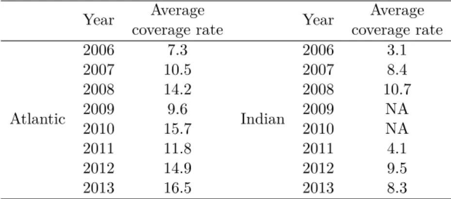
Table 1: Coverage rate of the french purse-seine fisheries in the Atlantic and Indian Ocean
Year coverage rateAverage Year coverage rateAverage
Atlantic 2006 7.3 Indian 2006 3.1 2007 10.5 2007 8.4 2008 14.2 2008 10.7 2009 9.6 2009 NA 2010 15.7 2010 NA 2011 11.8 2011 4.1 2012 14.9 2012 9.5 2013 16.5 2013 8.3
For most species, the fork length is preferred rather other length measurements. The fork length is the distance in a straight line from the tip of the nose to the fork of the
tail. For billfishes, the straight line starts from the tip of the lower jaw, for rays, the width is measured and for sharks or some fishes such as balistidae, observers measure the total length. All the length are taken at the centimetre below. Twenty random individuals (taken as a representative subsample) from the 100-150 sampled individuals are measured. When it is possible, the observer has to determine the sex of the individual. Observers sample bycatch species giving priority to certain species following the order below:
(i) Selachians - Sharks and Rays (ii) Turtles
(iii) Billfishes - Marlins, Sailfishes and Swordfishes (iv) Miscellaneous fishes
1.1.2 Data description
Data collected by observer trips (table 2) are organized in a R-data object with multiple tables ("tr" fishing trip details, "hh" fishing station details, "hl" samples, "sl" species details). The organization of the Rdata file is described by the entity diagram (Annex 2 -entity diagram). The sampling method is explained in a manual given to the observers which describes the different handling the observers have to do depending on what species occur in the net.
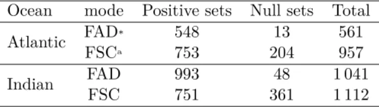
Table 2: Number of french purse-seine set sampled by observers program in the Atlantic and Indian Ocean. * Fish Aggregating DeviceaFree-Swimming Schools
Ocean mode Positive sets Null sets Total
Atlantic FADFSCa* 548753 20413 561957
Indian FADFSC 993751 36148 1 0411 112
Observers recorded the month, the time (hour/minutes), the ocean ("AtlOcean" for Atlantic Ocean, "IndOcean" for Indian Ocean) or more precisely the FAO area or the statistical square ("area" for the FAO fishing area, and "rect" for the 1¶x1¶ statistical
square), the type of fishing set ("FAD" or "FSC"), estimations of total weight of catch including bycatch ("wt" if it is from the logbook or "subSampWt" from the samples), length (subdivided in length classes of one centimetre each : "lenCls" ), geographic location of the fishing set (geographic coordinates "lonIni" and "latIni"), species or at least genus encountered ("spp"), the commercial category (discard "DIS" or landed "LAN"). There is an important inter-annual variability in terms of number of purse seine sets regardless of the ocean or the fishing method. We thus decided to conduct this work at the scale of the whole study period rather at a year scale (table 2). The amount of FAD sets in the Indian Ocean is twice higher than in the Atlantic Ocean, even if there was an interruption/reduction of any fishing activity in the Indian Ocean between 2009 and 2010. Seasons have been defined (warm season from December to May or cold season from June to November in the Atlantic and austral summer from October to march or austral winter April to September in the Indian Ocean).
1.2 Species composition and diversity indexes
In addition of studying the catch composition in terms of species list, using taxonomic richness, evenness and diversity indexes is a simple way to describe community and re-gional diversity.
1.2.1 Taxonomic richness, diversity and evenness A. Taxonomic richness
We estimated the richness in purse-seine sets by computing the taxonomic richness indexes
Sobs for all the modalities of the factors of interest (year, fishing mode). The best way to
compare taxonomic richness between different strates is to build rarefaction curves. Those curves are used first to show up the richness in a strate. Because hypothetical rarefaction curves should converge to an asymptote, we could use the curves build from the data to decide if there were enough sets to sample the total richness of the strate (asymptote reached or not) (Gotelli et al. 2001). Sample size (here the number of sets) strongly influences taxonomic richness. To deal with this bias, we applied a bootstrap procedure and randomly took with replacement 400 sets from the total number of sets in a modality of a given factor. This procedure was repeated 500 times and a Sboot,i was calculated for
all the samples i = 1, · · · , 500. Finally we computed the mean and standard deviation of the bootstrap samples Sboot,i for each modality and for all the factors of interest.
B. Taxonomic diversity and evenness
For practical and interpretational reasons, Simpson diversity and Simpson evenness in-dexes (⁄ and ESimpson) (Equations 1 and 2) were used to compare taxonomic diversity
and evenness among oceans and fishing methods (Hortal et al. 2006, Magurran 1988).
⁄ = 1 ≠ S i=1(p2i) (1) ESimpson = 1 ≠ D 1 ≠ 1 S (2)
With pi the proportion of biomass belonging to the ith species, S the number of present
species and D = S
i=1(p2i)
Where ⁄ is the probability for drawing randomly two different species, ESimpson is the
probability for drawing two different individuals. We tested then the significance of those indexes with variance analyses.
1.2.2 Species identification by ocean - species listing and grouping
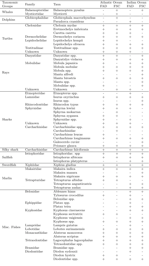
Maximising species richness is often an explicit or implicit goal of conservation studies. However, estimated species richness scores depend both on the estimator considered and on the grain size used to aggregate data (Gotelli et al. 2001). There were up to 114 taxa observed between the Atlantic and the Indian ocean (table 3) regardless of the fishing method.
Whales, dolphins and whale sharks are released before the closure of the net uninjured. However, observers estimated the weight of the animals encountered. Some turtles died in the net by suffocation because they got tided in the net. Silky sharks have been pulled out from the global group of sharks because of their emblematic and sensitivity to fishing despite their near-threatened status on the CITES list and frequency of occurrences in
Table 3: Taxa listing and presence/absence per ocean and fishing mode. (The presence in an ocean and under a fishing mode is symbolised by a + and absence with a -)
Taxonomic Family Taxa Atlantic Ocean Indian Ocean
Groups FAD FSC FAD FSC
Whales BalaenopteridaeMysticetidae Balaenoptera pysalusMysticeti -- ++ -- + -Dolphins Globicephalidae Globicephala macrorhynchusPseudorca crassidens -- +- +- -
-Turtles
Chelonidae Chelonia mydas + + + +
Eretmochelys imbricata + + + +
Caretta caretta + + +
-Dermochelidae Dermochelys coriacea + + + +
Lepidochelidae Lepidochelys kempii + + -
-Lepidochelys olivacea + + + + Testitudinae Testitudinae spp. + + + + Unknown Unknown + + + -Rays Dasyatidae Dasyatidae spp. + + - + Dasyatidys violacea + + + +
Mobulidae Mobula japanica + - + +
Mobula mobular + + + + Mobula spp. + + + + Manta alfredi - - - + Manta birostris + + + + Manta spp. - - - + Mobulidae spp. + - - + Unknown Unknown - + + -Sharks Etmopteridae Etmopterus spp. - - +
-Lamnidae Isurus oxyrinchus + + + +
Isurus spp. - - - +
Rhincodontidae Rhincodon typus + + + +
Sphyrnidae Sphyrna lewini + + +
-Sphyrna mokarran - + - -Sphyrna zyganea + + - -Sphyrnidae spp. + - + -Unknown Unknown + + + -Carcharhinidae Carcharhinidae spp. + + + + Carcharhinidae - + - -Carcharhinus leucas + - - -Carcharhinus longimanus + + + + Galeocerdo cuvier - - - + Prionace glauca + + + +
Silky shark Carcharhinidae Carcharhinus falciformis + + + +
Sailfish Istiophoridae Istiophoridae. sppIstiophorus albicans ++ ++ ++ ++
Istiophorus platypterus - - + +
Swordfish Xiphiidae Xiphius gladius + + + +
Marlin
Makairidae Makaira indica + + + +
Makaira mazara - - - +
Makaira nigricans + + + +
Tetrapturidae Tetrapturus albidus + + -
-Tetrapturus angustirostris - - + +
Tetrapturus audax - - + +
Misc. Fishes
Belonidae Ablennes hians - - + +
Tylosurus crocodilus + - +
-Belonidae spp. - - + +
Ephippidae Platax spp. - - +
-Platax teira - - + +
Kyphosidae Kyphosus cinerascens - - + +
Kyphosus sectratrix + + -
-Kyphosus vaigiensis - - + +
Kyphosus spp. + + + +
Lampridae Lampris gutatus - - +
-Lobotidae Lobotes surinamensis + + + +
Monacanthidae Aluterus monoceros + + + +
Aluterus scriptus + + + +
Tetraodontidae Lagocephalus lagocephalus + + + +
Tetraodontidae spp. + + + +
Bramidae Bramidae spp. - - + +
Diodontidae Diodon eydouxii - - +
-Diodon hystrix + + -
Taxonomic Family Taxa Atlantic Ocean Indian Ocean
Groups FAD FSC FAD FSC
Misc. Fishes
Exocoetidae Exocoetidae spp. + + + +
Serranidae Seriola rivoliana + + + +
Serranidae spp. - - +
-Sphyraenidae Sphyraena barracuda + + + +
Sphyraenidae spp. - - +
-Balistidae
Balistidae Abalistes stellatus - - + +
Balistes carolenensis + + -
-Balistes punctatus + - -
-Balistidae spp. + + + +
Canthidermis maculata + + + +
Molidae
Molidae Masturus lanceolatus + + + +
Mola mola + + + + Molidae spp. - - - + Ranzania laevis + + - -Carangidae Carangidae Carangidae spp. + + + + Carangoides orthogrammus - - + -Caranx crysos + + + + Caranx sexfasciatus - - + + Decapterus macarellus - - + -Decapterus spp. - - + + Naucrates ductor + + + + Uraspis helvola - - + -Uraspis secunda + + + + Uraspis spp. + - + -Uraspis uraspis - - + + Echeneidae
Echeneidae Phtheririchthys lineatus + + + +
Remora remora + + + +
Remorina albescens + + + +
Echeneis naucrates + + + +
Elagatis bipinnulata + + + +
Echeneidae spp. + + + +
Dorado Coryphaenidae Coryphaena equiselisCoryphaena hippurus ++ ++ ++ ++
Coryphaenidae spp. + - +
-Wahoo Scombridae Acanthocybium solandri + + + +
Auxis spp. Scombridae Auxis rocheiAuxis thazard ++ ++ ++ ++
Auxis spp. + + + +
Misc. Scombridae
Scombridae Euthynnus affinis + + + +
Euthynnus alletteratus + + + +
Sarda sarda + - -
-Scomber japonicus - - +
-Scombridae spp. - - +
-ALB Scombridae Thunnus alalunga + + + +
YFT Scombridae Thunnus albacares + + + +
SKJ Scombridae Katsuwonus pelamis + + + +
BET Scombridae Thunnus obesus + + + +
the net. Whale sharks haven’t been taken separately because there are just 13 sets with
Rhyncodon typus in the net and it has been released without any injuries. Whales and
dolphins occur in fishing operation report but are released safely and uninjured. Auxis spp. compared to Scombridae are dealt with separately because of their relative abun-dance compare to other small Scombridae.
The identification of the various taxa depends on how closed morphologically they are or on the ability of the observers to distinguish one taxon from another. Some bycatch species may have been grossly identified and were classified at genus or family level because of the difficulty to identify precisely some of them (33 taxa in 114). As a consequence to this, 22 taxonomic groups were developed. It helped to reduce the variability of the catch composition. Taxonomic groups help to smooth species identification issues by aggregat-ing captures.
1.3 Impact descriptors methodology
Additional criterions, other than richness, diversity and evenness indexes, have been used to compare the composition and changes of the taxonomic groups: length-class distribu-tion trophic and length-biomass spectrum amongst others.
1.3.1 Mean trophic level of the bycatch
The mean trophic level of the total catch and bycatch may help to understand the targeted part of the marine community structure. It is one of the most used indicators to describe the health of an ecosystem (Borcard et al. 2011). It gives a schematic illustration of the average composition of the studied community. The trophic level of each taxon has been resumed (Froese and Pauly 2014, Olson and Watters 2003) considering the maturity state (juvenile and adult) depending on the size of the individual. Then a geometric mean has been calculated among taxa of a same taxonomic group to give a mean trophic level of this group.
1.3.2 Length-class frequency of the bycatch
The length class distribution may be the easiest way to explore the range of size of the bycatch captured by a fishing mode. Size of the individuals are computed by fishing set in the subsample data of Obstuna and have been elevated to the whole fishing set using the ratio totalweighttaxa
sampleweighttaxa.
1.3.3 Biomass-size spectrum of the whole capture
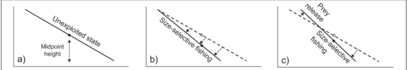
Biomass size spectra, the distribution of biomass across body size classes, appears to be a very conservative feature of marine communities. It summaries complex communities, comprising numerous species with complex trophic interactions, within a simple plot and two numbers: the slope (describing the exploitation rate of the ecosystem) and intercept (the accessible biomass) of the spectrum (Jul-Larsen et al. 2003). It allows also predictions of the effect of various human perturbations. It has been shown that linear biomass-size spectra are stationary solutions of the model. At the same time it was found that realistic fishing should affect the curvature and stability of the biomass-size spectrum rather than its slope. When there is no fishing activity, the spectrum is in a non impacted stationary state ( i.e. the slope of the spectrum is -1). Introducing a fishing activity will change the slope and the intercept of the spectrum or the amount of accessible biomass. Slopes (⁄) of log numbers versus log length have been ranged from -4 to -10 for weakly to heavily exploited fish communities (Benoît et al. 2003). In our case, we investigate the relation between log weight and log length and not log numbers versus log length, but there is a proportional relation between numbers and weight. The reasoning applies to any spectrum of this kind. According to Figure 1, three main stationary state could be possibly observed: non impacted stationary state, the fishing activity targets a specific size range but does not change the intercept (or the biomass accessible to the fishery) and a size-selective fishing which could occasionally release preys in the environment (both slope and intercept change).
There is a bias in the observer database: tuna are sampled only when they are dis-carded (so only the smallest ones are sampled). To correct that bias, we used the Balbaya database which corresponds to the sampling process conducted in the harbour at the land-ing. We then made the length classes corresponding to our fishing operations) because the sampling conducted in the harbour covers a whole boat slip and it is very difficult to tell to what fishing operation correspond a fish or another. There is a corrective process
Figure 1: How the biomass-size spectrum is modified from (a) an unexploited community, (b) alters as a results of size-selective fishing, and (c) potential prey release. (the dashed line: unexploited stationary state) (Jul-Larsen et al. 2003)
used for Balbaya which reduces that bias. By this operation, we reconstructed the length distribution for targeted tuna and corresponding biomass.
1.4 Explicative and predictive model of species composition and
abundance among space and seasons
1.4.1 Monospecific model
Silky sharks are mainly found in warm water in the Atlantic, Indian and Pacific Oceans. It is a large and slim shark growing up to a maximum length of 3.3 m. This shark is known to feed on bony fish such as tuna, mackerel, sardines and mullets.
Silky sharks occurred only in 161 sets on 1518 in the Atlantic ocean (11%) versus 704 sets on 2153 (32%) in the Indian Ocean. The captures data are zero inflated. A poisson distribution is more appropriated to low number of individuals where a negative binomial distribution is useful with rare high number of individuals. According to Figure 2, a zero-inflated Negative Binomial distribution ZINB with a logit-link function was selected to predict the presence/absence and number of Silky sharks caught (Amandé et al. 2011).
AtlOcean IndOcean 0 50 100 150 200 01 10 20 30 40 50 60 65 01 10 20 30 40 50 60 65 nSS count
Figure 2: Frequency distribution of silky sharks in purse-seine set per Oceans (captures are only from the french observers database and haven’t been elevated to the whole tuna fishery).
Parameters we decided to use in the model are: two spatial parameters (longitude and latitude), a temporal variable (the season) and the fishing mode. We will also extract the residuals from the ZINB and inspect these for any spatial correlation we could have forgotten in the model (Zuur et al. 2012). The zero inflated model fits two separate models: one to the zeros (absences) only, and the other to the counts. The mathematical equation for the model is:
Yi ≥ ZINB(µi, fii, ◊) (3)
log(µi) = —0+ —1.longitudei+ —2.latitudei+ —3.Seasoni+ —4.modei(4)
logit(fii) = “0+ “1.longitudei+ “2.latitudei+ “3.Seasoni+ “4.modei(5)
With E(Yi) = µi.(1 ≠ fii) and var(Yi) = (1 ≠ µi).µi.(1 + fii.µi+µ 2 i
◊ )
If we just consider a Negative Binomial distribution, its variance is given by the formula V = µi+ µ
2 i
◊ … V = µi+ –iú µ 2
i with –i = 1◊. ◊, —i, “i are unknown parameters
to estimate. If ◊ is large (◊ ∫ 0 … – ‘æ 0), the Negative Binomial distribution converge to a P oisson distribution. In the other way, when ◊ ‘æ 0, the variance is larger than in a
Poisson distribution and it was right to select a Negative Binomial distribution rather a Poisson’s.
1.4.2 Expansion of the model to the total catch composition
Diversity in purse-seine sets is an important component of the understanding of the impact of fishing activities on the ecosystem because it gives clues to determine how large is the community impacted. In their model, Oxbrough et al. (2005) investigated how spider communities change over forestation cycles in conifer and broadleaf plantations. They identified environmental and structural features of the habitat that can be used as indicators of spiders biodiversity. This model structure was used to describe how bycatch diversity changes across fishing methods and among oceans using structural, temporal and spatial parameters (Oxbrough et al. 2005 and Zuur, 2013). Inspired by this model, the objective was to determine what could affect the diversity in purse-seine sets . The effect of structural, temporal and spatial parameters on Simpson index among oceans and fishing methods were investigated. A General Addidive Model with a Binomial distribution
GAMbinomial with a logit-link function was selected to predict the value of the Simpson
index because of its range from 0 to 1. Parameters we decided to use in the model are: two spatial parameters (longitude and latitude), a temporal variable (the season) and the fishing mode. Residuals from the GAMbinomial were extracted and inspected for
any spatial correlation we could have forgotten in the model (Zuur et al. 2013). The mathematical equation for the model is:
Yi ≥ GAMbinomial(fii) (6)
logit(fii) = – + s(longitudei) + s(latitudei) + f(Seasoni) + f(modei) (7)
With E(Yi) = fii and var(Yi) = fii.(1 ≠ fii)
Because GAM models are non-parametric models, the smoothing splines approach the relation between the predictive variable and the explicative parameters (Maindonald, 2010).
2 Results
2.1 Descriptive approach
2.1.1 Distribution of purse seine set
The purse-seine sets are located in the Atlantic Ocean between 30¶ West to 12¶ East and
15¶ South to 20¶ North. For the Indian Ocean, the range of longitudes and latitudes
is: 40¶ West to 80¶ East and 21¶ South to 10¶ North (Figure 3). The spatial location
in the Atlantic Ocean has not really changed along years of the time series but changes along seasons. During the beginning of the warm season (from December to February), the fishing trips are conducted in the north of the Gulf of Guinea before moving offshore near the Senegal Coast at the end of the warm season (from march to may), then the prospection goes down to the extreme south of the Gulf of Guinea for the beginning of the cold season (from June to September) and then moves back inside the Gulf at the end of the cold season (from October to November). In the Indian Ocean, from December to march (austral summer), fishing sets are conducted in the Mozambican Channel and offshore of the Somalia coast before moving in the central part of the ocean from April to September (austral winter). In the Indian Ocean, fishing operations were disturbed in 2009 and 2010 by Somalian piracy and the number of observers onboard has been reduced to make place for marines (for the safety of the crew). As a consequence, in the Indian Ocean, there is a gap in the coverage rate and number of set between 2009 and 2010, period of the highest level of piracy.
● ● ●● ●●●●●● ● ● ● ● ● ● ● ● ●●● ● ●● ● ●● ●● ●● ● ● ● ● ● ●● ●● ● ● ● ●● ● ● ● ● ● ● ● ● ●● ● ● ●● ● ● ● ● ● ● ●● ● ● ● ● ● ● ●● ●● ● ●● ● ● ● ● ● ● ● ● ● ● ●● ● ● ●● ● ● ● ● ● ● ●● ● ● ● ●●● ● ● ● ● ● ● ● ● ● ● ●●● ● ● ● ● ● ● ●● ● ● ● ● ● ● ● ● ● ● ● ● ● ● ● ● ● ● ● ● ● ● ● ●● ● ● ● ● ● ● ● ● ● ● ● ● ●● ● ● ● ● ● ● ●●● ● ● ●● ● ● ● ● ● ● ● ● ●●● ● ● ●● ●●●● ●●●●● ● ● ● ●● ●●● ● ● ● ● ● ● ● ● ● ● ● ● ● ● ● ● ● ●● ● ● ● ● ● ● ● ● ● ● ● ● ●● ● ●● ● ● ● ● ● ● ● ● ● ● ● ● ● ●● ● ● ● ● ● ● ● ● ● ●●● ● ● ● ● ● ● ●●●●●●●●●● ● ● ●● ● ● ● ● ● ● ● ● ● ● ● ● ● ● ● ● ● ● ● ● ● ● ● ● ● ● ● ● ●●●●●● ● ● ● ● ● ● ● ● ● ● ● ● ●● ● ● ● ● ● ● ● ● ● ● ● ● ● ● ● ● ●● ● ● ● ● ● ● ● ● ● ● ● ● ● ●● ●●● ● ● ●● ● ● ● ●● ● ● ● ● ● ● ● ● ● ● ● ● ● ● ● ● ● ● ● ● ● ● ● ● ● ● ● ● ● ● ● ● ● ● ● ●●● ● ● ●● ●● ● ● ● ● ● ● ● ● ● ● ● ● ● ● ● ● ●●●● ● ●● ●●●●●●●●●●●●●●●●●●● ●●● ●● ● ● ● ● ● ● ● ● ● ● ● ● ● ● ● ● ● ● ● ●● ● ● ● ● ● ●●●●● ● ● ● ●● ● ●● ● ●● ● ● ● ● ● ● ● ● ●● ● ● ● ● ● ● ● ● ●● ● ● ●●●●●● ● ● ●● ● ● ● ● ● ●● ●●●●●●● ● ● ● ●● ● ● ● ●●●● ● ●● ● ● ● ● ● ● ●● ● ● ● ●● ● ● ● ● ● ● ●●● ● ● ● ● ● ● ● ● ● ● ●● ● ● ● ● ● ● ● ● ● ●● ● ● ● ● ● ● ● ● ● ● ● ● ● ●●●●● ● ● ●● ● ● ● ● ● ● ● ●●●●●● ● ● ● ● ● ● ●●●● ●● ●● ● ●● ● ● ● ● ● ●●● ● ● ●● ● ● ● ● ● ● ● ● ● ● ● ● ● ● ● ● ● ● ●● ● ● ● ●●● ● ●● ● ● ●●● ● ●● ● ● ● ● ● ● ● ● ● ● ● ● ● ● ●●● ● ● ● ● ● ● ● ● ● ● ● ● ● ● ● ● ●● ● ● ● ● ● ● ● ● ● ● ● ● ● ● ● ●● ● ● ● ● ● ● ● ●● ● ● ● ● ● ● ● ● ● ● ● ●●● ● ●●●● ● ● ● ● ●●●●●●●●●●● ● ● ●●●●●● ●● ●●●● ● ● ● ● ● ● ●●●● ● ● ● ● ●● ● ● ● ● ● ● ● ●● ● ● ● ● ● ● ● ● ● ● ● ● ● ● ● ● ●● ●● ● ● ● ● ● ● ● ● ● ● ● ● ●● ● ●●● ● ●●●●● ● ● ● ● ●● ● ● ● ●●●● ● ● ● ● ●●● ● ● ● ● ●●●● ● ●● ● ● ● ● ● ● ● ● ● ●● ● ● ● ● ● ●●●● ● ● ●● ● ● ● ● ● ● ● ● ● ● ●● ● ●● ● ● ● ● ● ● ● ● ● ● ● ● ● ● ● ● ● ● ● ● ● ● ● ● ●● ● ●●● ● ● ● ● ● ●● ● ● ● ● ● ●●● ● ● ● ● ●●●●●● ● ● ● ●●●● ● ● ● ●● ● ● ● ● ● ● ● ● ● ● ● ● ● ● ● ● ● ● ●●● ● ●●●●● ● ● ●●●●●● ●●●● ● ● ● ● ● ● ● ● ● ● ● ● ● ● ● ● ● ● ● ● ● ● ● ● ● ● ●●●●●●● ● ● ● ● ● ● ● ● ● ● ● ●●● ● ● ● ● ● ● ● ● ● ● ● ●●●●● ● ● ● ● ● ● ●●● ● ● ● ● ● ● ● ● ● ● ● ● ●● ● ● ●●● ● ● ● ● ● ● ● ● ● ● ● ● ●●●● ●● ● ● ● ● ● ●●●● ●● ● ● ● ● ●● ● ●● ●● ● ● ● ● ● ● ● ● ●● ● ● ● ● ● ● ● ● ● ● ● ● ● ● ● ●● ● ● ● ● ●● ● ● ● ● ●●●● ● ● ● ● ● ●● ● ● ●● ● ● ●●●●●●●●● ●●● ● ● ● ● ● ● ●●●●● ● ● ● ● ● ● ● ● ● ●●● ● ● ● ● ●● ● ●●● ● ● ●●● ● ●●● ● ● ● ● ●● ● ● ● ● ● ● ● ● ● ● ● ● ● ● ● ●● ● ● ● ● ●●● ●● ●● ● ●● ● ●● ● ● ● ● ●● ●●● ● ● ● ● ● ●● ● ● ● ● ● ● ● ● ●● ●●● ● ●● ● ●●● ●● ●● ●● ● ● ● ● ●●● ● ●● ● ● ● ● ● ● ● ● ●● ●●● ●● ● ● ● ● ● ●● ● ● ● ● ● ● ● ● ● ● ● ● ● ●●● ● ●●●●● ●●●●●●● ● ● ● ● ● ● ● ●●● ● ● ● ● ● ● ● ● ● ● ● ● ● ●● ● ● ● ● ● ● ● ● ●●● ●● ● ● ● ● ● ● ●●● ● ● ● ●●● ●● ● ● ● ● ●● ● ● ● ● ● ● ● ● ● ● ● ● ● ● ● ● ● ● ● ● ● ● ● ● ●● ● ● ● ●●●●● ● ● ●● ● ● ● ● ● ●●● ●●●●●●● ● ● ● ● ● ● ● ● ● ●● ● ● ● ● ●●● ● ● ● ● ●● ● ●● ●●●●● ● ●●●● ● ● ● ●● ● ●● ● ● ●●●● ● ● ● ● ●● ● ●●●●●●●●● ● ● ● ● ● ●●● ● ● ● ● ● ● ● ● ● ● ● ●● ●●● ● ● ● ●● ● ●●●● ● ●●●●● ● ● ●●● ● ● ● ● ● ● ● ● ● ● ● ● ● ● ● ● ● ● ● ●●● ●●●●●●●●●●●●●●●● ● ● ● ●●●●●●●●●●●●●●● ● ● ● ●●● ● ● ● ●●●● ●●●●●● ● ● ● ● ● ● ● ●●●●●●●● ● ● ●●● ● ● ● ●● ● ● ●●●● ●●●●●●● ● ● ● ● ●● ● ● ● ● ● ● ● ● ●● ● ●● ●● ● ● ● ● ● ●●●●●●● ● ● ● ● ●●●● ● ●●● ● ● ●●● ● ● ● ● ● ●● ●●●● ● ● ●●● ● ● ● ● ● ● ● ● ● ● ● ● ●● ● ●●●●●● ● ● ● ●●● ● ● ● ● ● ●●● ● ● ● ● ● ● ● ● ● ● ● ● ● ● ● ● ● ● ● ● ● ● ● ● ● ●●●● ● ● ●● ● ● ●● ● ● ● ● ● ● ● ● ● ●●●● ● ● ● ● ●●● ●● ● ● ● ● ● ● ●● ● ●●●● ● ● ● ● ●● ● ● ● ● ● ●● ●●●●●● ● ● ● ● ● ● ● ● ●● ● ● ● ● ● ● ●● ● ● ● ● ● ●● ● ● ● ● ● ● ● ● ● ● ● ● ● ● ● ● ● ● ● ● ● ● ● ● ● ● ● ● ● ● ● ● ● ● ● ● ● ● ● ● ● ● ● ● ●●●●●●●●●● ●●● ● ●●●●●●●●●● ● ● ● ● ● ●● ● ● ● ● ● ● ●●● ● ● ● ● ● ● ●● ● ● ● ● ●●●● ● ● ● ● ● ● ● ● ● ● ● ● ● ● ● ● ●● ● ●● ● ● ●●●● ● ● ● ● ● ● ● ● ● ● ● ● ● ● ● ● ●● ● ●● ● ● ● ● ●●●●●●●●● ● ● ●● ● ● ● ● ● ● ●●●●● ● ● ● ● ● ● ● ● ● ● ● ● ● ● ●●●●●●●●●●●●●●●●●●● ● ● ● ● ● ● ● ● ● ● ● ● ● ● ● ● ● ● ● ●●●●●●● ● ● ● ● ● ● ● ●●●● ● ● ●●●●● ●● ● ●●●●●● ● ● ● ● ●● ● ● ●●●●● ● ● ● ●● ● ● ● ● ● ● ●● ● ● ● ● ● ● ● ●● ● ● ● ● ●●● ● ● ● ● ● ● ● ●●● ● ● ● ●●● ● ●●●●● ●● ●●● ● ● ● ● ●● ● ● ● ● ● ●●● ● ● ● ● ● ● ● ●● ● ● ●● ● ● ● ●● ● ● ● ● ● ● ● ●● ● ● ● ● ● ●●●●●●●●● ● ● ● ● ● ● ● ● ●●●●●●● ●● ●●●●●●● ● ● ● ●●● ● ● ●● ● ● ● ● ● ● ● ●● ● ●●●● ●●●● ● ● ●●●●●● ● ● ●●●●●●●●●● ● ● ● ●●●●●● ● ● ●● ●●●●●● ● ● ● ●● ● ●●●● ● ● ● ● ● ● ● ● ● ● ● ● ●● ●●● ●●●●●● ● ●● ● ●● ●●●● ● ● ● ● ● ● ● ● ● ● ● ● ● ● ● ●● ● ● ● ● ● ● ● ● ●● ● ● ● ● ● ● ●● ● ● ● ● ● ●●●●●●●●●● ●●● ●●●●●●●●●● ● ● ●●● ● ●● ● ● ● ● ● ● ●●● ● ● ●● ●● ● ● ● ● ● ● ●●●●● ●●●● ● ● ● ● ● ● ●●● ● ● ● ● ●●● ● ● ● ● ● ● ●● ●● ●● ● ● ● ● ● ● ●● ● ● ● ● ● ●●●●●●●●●● ● ● ● ● ● ● ● ● ● ● ● ● ●●●●●●●●●●● ● ● ● ● ● ● ●●●●● ●●●●●●●●●● ● ● ● ●●●● ●● ● ● ● ●●● ●●●●●●●● ● ● ●● ●●●●●●●●●● ●● ● ● ● ● ● ● ● ● ● ● ● ● ● ● ●●● ● ● ●●● ●● ●●●●●●●●●●●●●●● ● ● ● ● ●● ● ● ● ● ● ● ● ● ● ● ● ● ● ● ●● ●● ●● ● ● ● ● ● ● ● ● ● ● ● ●●●●●●● ● ● ● ●●●●●●●●●●●●●● ●● ● ● ● ● ● ● ● ● ●●●● ●● ● ● ● ● ● ●● ●●● ●●● ●● ● ● ● ●● ● ● ● ● ● ● ● ●●● ●●●●●●●●●● ● ● ● ● ●● ● ●● ● ●●●●●●● ● ● ● ● ● ● ● ● ●●●●● ● ● ●● ● ● ● ● ● ● ● ●● ● ● ● ● ● ● ● ● ●● ● ● ● ● ●●● ●● ● ● ● ● ●●● ● ● ● ● ● ● ● ● ● ● ● ●● ● ● ● ● ● ● ● ● ● ● ●● ● ●● ● ●● ● ●●●●● ●● ●● ● ● ● ● ● ● ● ● ● ● ● ● ● ● ● ● ●● ● ● ● ● ● ● ● ● ●●● ● ● ● ● ● ● ● ● ●● ● ● ● ● ● ● ● ● ● ● ● ● ● ● ● ● ● ● ● ● ●● ● ● ● ● ● ● ● ● ● ● ● ● ● ● ● ●●●●●●●● ● ● ● ● ● ● ● ●● ●● ●● ● ● ● ●●● ● ● ● ● ● ● ● ●● ● ●●● ● ● ● ● ● ● ● ● ●● ● ● ●●●●●● ●●●●●● ● ● ●●●● ● ●●● ● ● ● ● ● ● ● ●● ● ● ● ● ●●● ● ● ● ●●● ● ●●●● ● ● ● ● ● ● ● ● ● ● ●●●● ● ●●● ● ● ● ● ● ● ● ● ● ● ● ● ● ● ● ● ● ● ● ● ●● ●● ● ● ● ●●●● ● ●● ●●●● ●● ● ● ● ● ● ● ● ● ● ● ● ● ●●●●● ●●●●●●●● ● ● ● ● ● ● ● ● ● ●● ● ● ● ● ● ● ● ● ● ● ●●●●●● ● ● ● ● ●● ● ● ● ● ● ● ● ● ● ●● ● ● ● ●●●● ● ● ●● ● ● ● ●● ● ● ● ●●● ● ● ● ●● ● ● ● ● ● ●●●●●●● ● ● ● ●● ●●●● ● ● ● ● ●● ● ● ● ● ●●● ● ● ●● ● ● ● ● ● ● ● ● ● ● ● ● ● ● ●● ●●●●● ● ● ● ●●●●● ● ●●●●●● ● ● ● ● ● ● ● ●●● ● ● ● ● ● ● ● ● ● ● ● ● ● ● ● ● ● ● ● ● ●●●● ● ● ●●● ● ● ●●●● ●●●●●●●●●● ● ●●● ● ● ● ● ● ●●● ● ● ● ● ●●●●●●● ● ● ●● ● ● ● ● ●●●●● ● ● ● ● ● ● ● ●● ● ● ● ● ● ● ● ● ● ● ● ● ● ● ●●● ● ● ● ● ● ●● ● ● ● ● ● ● ● ●●●● ● ● ● ● ● ● ● ● ●● ● ● ● ● ● ● ● ● ● ● ● ● ● ● ● ● ● ● ● ● ●●●● ● ● ● ● ●●● ● ● ● ● ● ●● ● ● ● ● ● ●●● ●● ● ● ● ● ● ● ● ● ● ● ● ● ●● ● ● ● ● ● ● ● ●● −20 −10 0 10 20 −30 0 30 60 lonIni latIni
Figure 3: Purse-seine FAD and FSC set in the Atlantic and Indian Ocean from 2006 to 2013 ( underFADin red and underFSCin blue)
2.1.2 Catch over Oceans and fishing methods
Discards are much higher under FAD (table 4). Captures are higher in the Indian Ocean regardless to the fishing mode due to the lower number of set in the Atlantic Ocean compared to the Indian Ocean. Furthermore, in the Atlantic Ocean, captures under FAD are slightly lower than in FSCs. It is the contrary in the Indian Ocean where captures are slightly higher under FAD.
Table 4: Landings and discards proportion and amount under FAD and FSC among oceans (captures are only from the french observers database and haven’t been elevated to the whole tuna fishery).
Atlantic Ocean Indian Ocean
FAD FSC FAD FSC
Discards (t) 1 409 425 1 504 778
Landings (t) 11 745 17 464 22 743 19 928
Discards (%) 10.71 2.38 6.39 3.76
2.1.3 Richness, diversity and evenness indexes
On the 114 taxa, a total of 68 taxa were common to both oceans (table 5), 13 exclusive to the Atlantic (such as Tetrapturus albidus and Kyphosus sectatrix) and 34 to the Indian ocean (such as Galeocerdo cuvier or Manta alfredi).
Table 5: Exclusive and common taxa over fishing modes and oceans.
Atlantic Ocean Indian Ocean
FAD FSC FAD FSC
Exclusive Taxa per fishing mode 2 4 13 5
Exclusive taxa per ocean 13 34
Taxa in common between fishing mode 62 63
Taxa in common between oceans 68
Total number of taxa 68+13 = 81 68+34 = 102
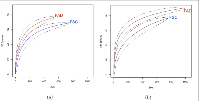
Rarefaction curves have been constructed by ocean and fishing mode (figure 4). The FAD rarefaction curve converges in the Atlantic ocean to an asymptotic value of 80 taxa where the FSC rarefaction curve converges to 70. In the Indian Ocean, the asymptotic value under FAD is 90 and under FSC it is 75 (captures are only from the french observers database and haven’t been elevated to the whole tuna fishery).
The bootstrap procedure had for result an estimation of both the richness and the uncertainty of measurement (table 6). As expected, richness under FAD is higher than in FSC. Moreover, richness is higher in the Indian Ocean than in the Atlantic Ocean.
Table 6: Estimated richness from bootstrap (400 samples and 500 iterations).
Atlantic Ocean Indian Ocean
FAD FSC FAD FSC
Richness 66 57 74 58
Ecart type ± 2.5 ± 2.9 ± 3 ± 3.6
Both Simpson diversity and Simpson evenness indexes are higher under FAD than under FSC for a given ocean (figure 5 and table 7). The value of those indexes under FAD is significantly higher in the Indian Ocean (anova with a p-value<5%). Captures under FSC are often monospecific. As a consequence of that, the value of the Simpson diversity and evenness indexes are 0. It explains the box plot sprawl under FSC. Fishing under FAD impacts a larger range of the species spectrum.
0 200 400 600 800 1000 0 20 40 60 80 Atl Sets NB Species (a) 0 200 400 600 800 1000 0 20 40 60 80 Ind Sets NB Species (b)
Figure 4: The rarefaction curves for the Atlantic Ocean (a) and the Indian Ocean (b) (FAD
in red andFSCin blue) shows sample-based rarefaction and asymptotic richness for the different
fishing mode in both oceans.
● ● ● ● ● ● ● ● ● ● ● ● ● ● ● ● ● ● ● ● ● ● ● ● ● ● ● ● ● ● ● ● ● ● ● ● ● ● ● ● ● ● ● ● ● ● ● ● ● ● ● ● ● ● ● ● ● ● ● ● ● ● ● ● ● ● ● ● ● ● ● ● ● ● ● ● ● ● ● ● ● ● ● ● ● ● ● ● ● ● ● ● ● ● ● ● ● ● ● ● ● ● ● ● ● ● ● ● ● ● ● ● ● ● ● ● ● ● ● ● ● ● ● ● ● ● ● ● ● ● ● ● ● ● ● ● ● ● ● ● ● ● ● ● ● ● ● ● ● ● ● ● ● ● ● ● ● ● ● ● ● ● ● ● ● ● ● ● ● ● ● ● ● ● ● ● AtlOcean IndOcean 0.00 0.25 0.50 0.75 FAD FSC FAD FSC year Simpson Div ersity Inde x
Simpson Diversity index per year and fishing mode and Ocean
(a) ● ● ● ● ● ● ● ● ● ● ● ● ● ● ● ● ● ● ● ● ● ● ● ● ● ● ● ● ● ● ● ● ● ● ● ● ● ● ● ● ● ● ● ● ● ● ● ● ● ● ● ● ● ● ● ● ● ● ● ● ● ● ● ● ● ● ● ● ● ● ● ● ● ● ● ● ● ● ● ● ● ● ● ● ● ● ● ● ● ● ● ● ● ● ● ● ● ● ● ● ● ● ● ● ● ● ● ● ● ● ● ● ● ● ● ● ● ● ● ● ● ● ● ● ● ● ● ● ● ● ● ● ● ● ● ● ● ● ● ● ● ● ● ● ● ● ● ● ● ● ● ● ● ● ● ● ● ● ● ● ● ● ● ● ● ● ● ● ● ● ● ● ● ● ● ● ● AtlOcean IndOcean 0.00 0.25 0.50 0.75 1.00 FAD FSC FAD FSC year Simpson Ev enness Inde x
Simpson Evenness index
(b)
Figure 5: Simpson diversity index (a) and Simpson evenness index (b) in the Atlantic and Indian Ocean
Table 7: Estimated diversity and Evenness per oceans and fishing mode.
Atlantic Ocean Indian Ocean
FAD FSC FAD FSC
Diversity 0.7814 0.3266 0.8363 0.3245 Evenness 0.8031 0.3376 0.8547 0.3358
2.1.4 Typical fishing set species composition profile
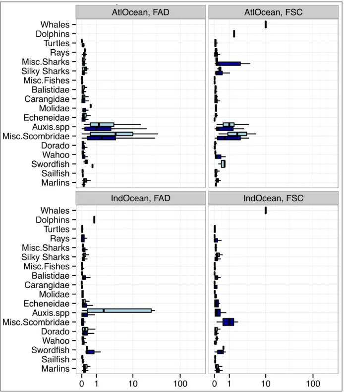
In terms of numbers of occurrences, the taxonomic composition reveals differences between oceans and fishing modes (table 8). Sailfishes are more present in FSC rather in FAD
FAD FSC FAD
contrary to marlins which occur more frequently under FAD. Rays are more frequently observed in FSC and sharks (miscellaneous and Silky sharks independently) under FAD. Table 8: Group listing and occurrences per ocean and fishing mode (captures are only from the french observers database and haven’t been elevated to the whole tuna fishery).
Category Group Taxonomicgroups Atlantic Ocean Indian OceanFAD FSC FAD FSC
bycatch Cetaceans Whale 0 8 0 3 Dolphins 0 1 1 0 Turtles Turtles 25 35 17 6 Selachians Rays 19 39 57 87 Misc. sharks 47 36 68 20 Silky sharks 118 43 647 57 BillFishes Marlins 94 44 161 82 Sailfishes 34 158 28 21 Swordfishes 5 3 9 3
Fishes Misc. Fishes 273 81 730 65
Balistidae 368 42 753 49 Molidae 13 28 4 9 Carangidae 332 34 275 10 Echeneidae 349 64 703 53 Dorado 274 44 747 53 Wahoo 310 42 640 39 Misc. Scombridae 93 8 59 3 Auxis spp. 164 15 428 44 Target spp. Tuna ALB 4 15 17 106 YFT 317 597 875 594 SKJ 498 149 922 150 BET 163 94 388 138
Landings and discards data have been summarized by ocean, fishing method (FAD or FSC) and species or group of species. The amount and composition of catches vary among oceans and fishing methods. All the 22 species groups are caught in both oceans but most species caught are different. Catch per set and taxonomic group were plotted (Figure 6) among fishing methods, oceans. While considering a specific Ocean, some species groups are predominant in the catch depending on the fishing method. In the Atlantic Ocean, the most common groups encountered under FAD are: Auxis spp., Misc. Scombridae and various fishes such as Balistidae and Carangidae ; while under FSC, the main groups are: Auxis spp., misc. Scombridae, Sailfishes and Wahoo. In the Indian Ocean, under FAD it is common to observe more sharks and mesopelagic fishes like Balistidae, Echenidae and Dorado while under FSC there are more Billfishes, Misc. Scombridae, Carangidae and Rays. It is in accordance with the table 8 summarising the occurrences of each taxonomic groups.
AtlOcean, FAD AtlOcean, FSC
IndOcean, FAD IndOcean, FSC
Marlins Sailfish SwordfishWahoo Dorado Misc.ScombridaeAuxis.spp Echeneidae Molidae CarangidaeBalistidae Misc.Fishes Silky Sharks Misc.SharksRays Turtles DolphinsWhales Marlins Sailfish Swordfish Wahoo Dorado Misc.Scombridae Auxis.spp Echeneidae Molidae Carangidae Balistidae Misc.Fishes Silky Sharks Misc.Sharks Rays Turtles Dolphins Whales 0 1 10 100 0 1 10 100
catch (t/year) log−scale
species group
catchCat
DIS LAN
catch per set under FAD in the Atlantic Ocean
Figure 6: Purse-seine FAD and FSC catch (t/set) in the Atlantic and Indian Ocean per species group (Discardsin dark blue andlandingsin blue)(captures are only from the french observers
2.2 Indicators of the fishery impacts
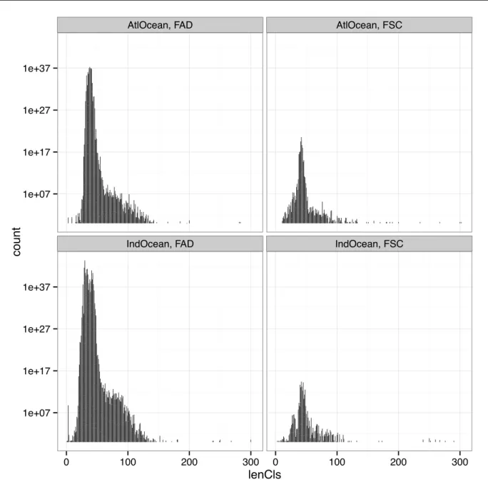
2.2.1 Length-class distribution of the bycatch
The length class distribution of the bycatch community has been plotted (figure 7). There is no significant difference between oceans and fishing mode (p-value > 5%). But on FSC it seems that the length class distribution is slightly broken down in two modes: one around 50 cm and the second around 80 cm. On FAD the length class distribution is smoother and if two modes should be viewed, the first one is around 35 cm and the second around 70-80 cm. In short, therefore, it appears that, even if it is not significant, length class are shifted to smaller distributions under FAD.
AtlOcean, FAD AtlOcean, FSC
IndOcean, FAD IndOcean, FSC 1e+07 1e+17 1e+27 1e+37 1e+07 1e+17 1e+27 1e+37 0 100 200 300 0 100 200 300 lenCls count
Figure 7: Length class spectrum of the bycatch under FAD and FSC in the Atlantic and Indian Ocean (captures are only from the french observers database and haven’t been elevated to the whole tuna fishery).
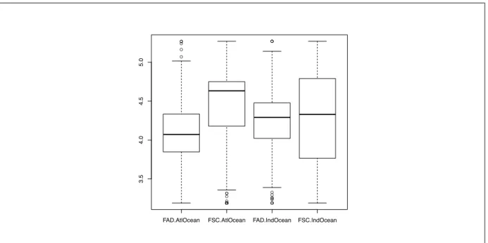
2.2.2 Mean Trophic Level of the bycatch
The mean trophic level appeared to be quite different from FAD to FSC (figure 8). Indeed, a Kruskal-Wallis test has been done and shows up significant difference between fishing mode for a given ocean (table 9). The median of trophic level in the Atlantic Ocean is 4.07 under FAD and 4.63 on FSC, where in the Indian Ocean the median trophic level is 4.29 under FAD and 4.33 on FSC.
● ● ● ● ● ● ● ● ● ● ● ● ● ● ● ● ● ● ● ● ● ● ● ● ● ● ●● ● ● ● ● ● ● ● ● ● ●
FAD.AtlOcean FSC.AtlOcean FAD.IndOcean FSC.IndOcean
3.5
4.0
4.5
5.0
Figure 8: Mean trophic level per set for both oceans and fishing mode
The difference in mean trophic level between fishing mode is strongly significant in the Atlantic ocean but slightly significant in the Indian Ocean (table 9).
Table 9: Kruskal-Wallis test on trophic level.
Atlantic Ocean Indian Ocean
FAD FSC FAD FSC
median trophic level 4.07±0.03 4.63±0.05 4.29±0.02 4.33±0.09
kruskal wallis test ˙p value <˝¸2.2e ≠ 16˚ ˙p value˝¸= 0.01232˚
2.2.3 Biomass-size spectrum
Slopes of the biomass-size spectrum (figure 9) are always higher under FAD (slopes ranged from ≠12 to ≠15 for respectively the Atlantic and the Indian Ocean) than under FSC (slopes ranged from ≠6.5 to ≠9.9 for respectively the Atlantic and the Indian Ocean). The impact on the overall community size structure of a fishing mode appears to be mostly higher under FAD. Although the means of biomass-size distribution (intercepts) are higher under FAD too. It means that the amount of total accessible biomass is not the same depending on the fishing fishing mode (fishermen don’t exploit the same part of the overall marine community).
The spectra in the Indian Ocean cross themselves for a log-length of 4.70 which corre-sponds to a length class of 109 cm. It could mean that the fishing pressure is mostly on fishes longer than 109 cm and that smaller fishes (under 109 cm) are mostly discarded or released. The spectra in the Atlantic Ocean cross themselves for a log-length of 5.05
which corresponds to a length class of 161 cm. It could mean that the fishing pressure is mostly on fishes longer than 161 cm and that smaller fishes (under 161 cm) are mostly discarded or released. The impact of the tuna purse-seine fishery seems to be higher in the Indian ocean than in the Atlantic ocean
● ● ● ● ● ● ● ● ● ●● ● ● ● ● ● ● ●●● ● ● ●● ●●●● ●● ●● ● ● ●● ● ● ● ● ● ● ● ● ● ● ● ● ●● ●● ● ●● ● ● ● ● ●● ● ● ● ● ● ● ● ● ● ●● ●● ● ● ● ● ● ● ● ● ● ● ● ● ● ● ● ● ● ● ●● ● ● ● ● ● ● ● ● ● ●● ● ● ● ● ● ● ● ● ● ● ● ● ● ● ● ● ● ● ● ● ●● ● ● ● ● ● ● ● ● ● ● ● ● ● ●● ● ● ● ●●● ● ●●●● ● ● ● ●● ● ● ● ● ● ●●● ●● ● ● ● ● ● ● ●● ● ● ● ● ● ● ● ●● ● ● ● ● ● ● ● ● ● ● ●● ● ●●● ● ● ● ● ● ● ● ● ● ● ● ● ●● ● ● ● ● ● ● ● ● ● ●● ● ●● ●●● ● ● ● ● ● ● ● ● ● ● ● ● ● ● ● ● ● ● ●●●●● ● ● ●● ●● ●● ● ●● ●●● ● ● ●● ● ●●●● ●●●● ● ●● ●●● ● ● ● ● ● ●● ●● ● ● ● ● ● ●● ● ● ●● ● ● ●● ● ● ● ● ● ● ● ● ● ● ● ●● ● ●●● ● ● ● ● ● ● ● ● ● ● ● ● ● ● ● ● ● ● ● ●●● ● ●● ● ● ● ● ● ●● ● ● ● ● ●● ● ● ● ● ● ● ● ● ● ● ● ● ● ● ● ● ● ●●● ● ● ● ● ● ● ● ● ● ● ● ●● ● ● ● ● ● ● ● ● ● ● ● ● ● ● ● ● ● ● ● ● ●● ● ● ● ● ● ● ● ● ● ● ●● ● ● ● ● ● ● ● ● ● ●● ● ● ● ● ● ● ● ● ● ● ● ● ● ● ● ● ●● ● ● ● ●● ● ● ● ● ● ● ● AtlOcean IndOcean 10 20 30 3 4 5 3 4 5 log(length) Log(wt)
Figure 9: Biomass by length class spectrum (FAD in red full line andFSCin blue dashed line)(captures
are only from the french observers database and haven’t been elevated to the whole tuna fishery).
Equations of the spectra are:
log(WF ADAtl ) = 70 ≠ 12.log(LAtlF AD); r2 = 0, 838 (8) log(WF SCAtl ) = 42 ≠ 6.5.log(LAtlF SC); r2 = 0, 549 (9) log(WF ADInd ) = 86 ≠ 15log(LIndF AD); r2 = 0, 825 (10) log(WF SCInd ) = 62 ≠ 9.9.log(LIndF SC); r2 = 0, 513 (11)
FAD
FSC
FAD