REVIEW ARTICLE
Standard epidemiological methods to understand and
improve
Apis mellifera
health
Dennis vanEngelsdorp
1*, Eugene Lengerich
2, Angela Spleen
2, Benjamin Dainat
3, James Cresswell
4,
Kathy Baylis
5, Bach Kim Nguyen
6, Victoria Soroker
7, Robyn Underwood
1, Hannelie Human
8, Yves Le
Conte
9and Claude Saegerman
101Department of Entomology, 3136 Plant Sciences, University of Maryland, College Park, MD 20742, USA.
2Department of Public Health Sciences, College of Medicine, The Pennsylvania State University, Hershey, PA, 17033, USA.
3Swiss Bee Research Centre, Agroscope Liebefeld-Posieux ALP-Haras, Schwarzenburgstrasse 161, 3003 Bern, Switzerland.
4Biosciences, College of Life & Environmental Sciences, University of Exeter, Hatherly Laboratories, Prince of Wales Road,
Exeter, EX4 4PS, UK.
5Department of Agriculture and Consumer Economics, University of Illinois, Urbana, IL 61801, USA.
6Department of Functional and Evolutionary Entomology, University of Liege, Gembloux Agro-Bio Tech, B-5030 Gembloux,
Belgium.
7Department of Entomology, Agricultural Research Organization, The Volcani Center P.O.B. 6, Bet Dagan 50250, Israel.
8Department of Zoology and Entomology, University of Pretoria, Pretoria, South Africa.
9INRA, UR 406 Abeilles et Environnement, Site Agroparc, Domaine St Paul, 84914 Avignon Cedex 9, France.
10Research Unit in Epidemiology and Risk Analysis Applied to Veterinary Sciences (UREAR-ULg), Department of Infectious and
Parasitic Diseases, Faculty of Veterinary Medicine, University of Liège, Boulevard de Colonster 20, B42, 4000 Liège, Belgium.
Received 1 June 2012, accepted subject to revision 10 August 2012, accepted for publication 26 October 2012.
*Corresponding author: Email: dennis.vanengelsdorp@gmail.com
Summary
In this paper, we describe the use of epidemiological methods to understand and reduce honey bee morbidity and mortality. Essential terms are presented and defined and we also give examples for their use. Defining such terms as disease, population, sensitivity, and specificity, provides a framework for epidemiological comparisons. The term population, in particular, is quite complex for an organism like the honey bee because one can view “epidemiological unit” as individual bees, colonies, apiaries, or operations. The population of interest must, therefore, be clearly defined. Equations and explanations of how to calculate measures of disease rates in a population are provided. There are two types of study design; observational and experimental. The advantages and limitations of both are discussed. Approaches to calculate and interpret results are detailed. Methods for calculating epidemiological measures such as detection of rare events, associating exposure and disease (Odds Ratio and Relative Risk), and comparing prevalence and incidence are discussed. Naturally, for beekeepers, the adoption of any management system must have economic advantage. We present a means to determine the cost and benefit of the treatment in order determine its net benefit. Lastly, this paper presents a discussion of the use of Hill’s criteria for inferring causal relationships. This framework for judging cause-effect relationships supports a repeatable and quantitative evaluation process at the population or landscape level. Hill’s criteria disaggregate the different kinds of evidence, allowing the scientist to consider each type of evidence individually and objectively, using a quantitative scoring method for drawing conclusions. It is hoped that the epidemiological approach will be more broadly used to study and negate honey bee disease.
Métodos estándar epidemiológicos para entender y mejorar la
salud de
Apis mellifera
Resumen
En este trabajo se detalla el uso de métodos epidemiológicos para entender y reducir la morbilidad y la mortalidad de las abejas. Se presentan y definen algunos términos esenciales y también se ponen ejemplos de su uso. La definición de términos tales como enfermedad, población, Journal of Apicultural Research 52(1): (2013) © IBRA 2013 DOI 10.3896/IBRA.1.52.1.08
Footnote: Please cite this paper as: VANENGELSDORP, D; LENGERICH, E; SPLEEN, A; DAINAT, B; CRESSWELL, J; BAYLISS, K; NGUYEN, B K; SOROKER, V;
UNDERWOOD, R; HUMAN, H; LE CONTE, Y; SAEGERMAN, C (2013) Standard epidemiological methods to understand and improve Apis mellifera health. In V Dietemann; J D Ellis, P Neumann (Eds) The COLOSS BEEBOOK: Volume II: Standard methods for Apis mellifera pest and pathogen research.Journal of Apicultural Research 52(1): http://dx.doi.org/10.3896/IBRA.1.52.1.08
sensibilidad y especificidad, proporciona un marco de referencia para las comparaciones epidemiológicas. El término población, en particular, es muy complejo en un organismo como la abeja de la miel, porque uno puede ver la "unidad epidemiológica" como las abejas individuales, las colonias, los colmenares o incluso, determinadas operaciones. La población de interés debe, por lo tanto, estar claramente definida. Se proporcionan además ecuaciones y explicaciones sobre cómo calcular las medidas de la tasas de enfermedad en una población.
研究和改善西方蜜蜂健康的标准流行病学研究方法
本文详述了如何应用流行病学的研究方法,探明和降低蜜蜂发病率及死亡率。同时还对一些关键术语进行了定义,并举例和说明了它们的用途。 定义了诸如:疾病、群体、敏感性和特异性等术语,为流行病学比较研究提供了框架。“群体”的含义在蜜蜂学研究中是比较复杂的,研究者可将 一个蜜蜂的个体、一个蜂群、一个蜂场或某项实验定义为一个 “流行病学研究单位”。所以,在开展流行病学研究时必须对所研究的群体加以明 确定义。本文还阐述了如何评价群体的发病程度,并给出了相关的计算公式和注解。
Key words: COLOSS, BEEBOOK, honey bee Apis mellifera, epidemiology, disease, case definition confidence interval, odds ratio, relative risk, Hills Criteria
1. Basic epidemiological terms and
calculations
Epidemiology is traditionally defined as the study of the distribution and determinants of disease within a human population (Woodward, 2005). To accomplish this, epidemiological studies attempt to identify factors which may explain or contribute to disease outbreak. Once identified, these factors not only inform future clinical etiological studies, but also, and perhaps more importantly, they inform disease prevention and control programmes (Mausner and Kramer, 1985). The success of epidemiologists in reducing the occurrence of human disease over the last century is undeniable. The identification of factors that contribute to the occurrence of diseases such as lung cancer (smoking), sexually transmitted diseases (unprotected sex), and cardiovascular disease (high blood pressure) have permitted targeted community health initiatives aimed at preventing or controlling risk factor exposure. These initiatives, in turn, have helped reduce the rate of disease in targeted populations (Mausner and Kramer, 1985; Koepsell and Weiss, 2003; Woodward, 2005).
Considering the success of human epidemiology, it is not surprising that epidemiological methods have been adopted by those wishing to understand and reduce disease outbreak in non-human animals (epizootiology) (Nutter, 1999). The term epidemiology is now widely adopted by those studying disease and disease determinants in non-human organisms, including honey bees, and will be the term used in this paper. Nutter (1999) argued that the application of epidemiological methods for understanding disease occurrence in plant, human, and animal populations involves the implementation of six common steps which include defining disease in quantitative terms and quantifying state and rate variables of the disease system. An alternative way to look at this process is to consider the "virtuous epidemiological cycle" (Fig. 1) which outlines the various steps involved in quantifying disease in a population, determining risk factors contributing to disease occurrence, determining methods to
reduce disease occurrence and then evaluating the effectiveness of these methods (Toma et al., 1991).
A comprehensive review of all of these steps is well beyond the scope of this paper. Similarly, much of the data used by
epidemiologists are derived from surveillance efforts, a discussion of which is also beyond the scope of this paper, but has received attention in other recent work (Hendrikx et al., 2009, vanEngelsdorp et al., 2013). Instead, we focus on presenting and defining the vocabulary needed to implement epidemiological studies, and then outline study design, analysis and interpretation. It is also the intent of this paper to present a framework for understanding and initiating ongoing and future studies of honey bee health. Unless otherwise noted, the following terms and concepts have been adapted from Koepsell and Weiss (2003).
Fig. 1. The virtuous circle of epidemiology: Step 1. describe health characteristics of the population in space and time (descriptive epidemiology); Step 2. analyse data and mechanisms of development of the disease to understand behaviour (analytical epidemiology); Step 3. produce, select and apply control or preventive measures (operational epidemiology); Step 4. give necessary information that permits the follow up of measures (evaluative epidemiology); In addition, changing epidemiological methods should be supported by theoretical epidemiology (modelling).
1.1. Disease
To successfully develop tools which either quantify the rate of disease development in a population or quantify the factors which may contribute to disease occurrence, the “disease” of interest must be clearly defined. Broadly speaking, disease is any departure from perfect health. When applied to specific studies, a precise definition - the case definition - must be developed which unambiguously allows subjects to be classified as a case or not.
1.1.1. Case definition
The case definition is the operating definition of a disease for study purposes. Aristotle identified two crucial components that made for a good case definition: 1. it specifies characteristics common to all diseased individuals; and 2. it specifies how diseased individuals differ from non-diseased individuals (Koepsell and Weiss, 2003). Ideally, the characteristics used to identify the disease should be simple and recognizable by independent observers in different geographies. Because characteristics cannot always be recognized in the field, case confirmation by laboratory analyses is sometimes necessary. Case definitions, especially for emerging or newly identified diseases, often suffer from having limited specificity. Further, case definitions for a disease can evolve as understanding of a disease changes and / or the diagnostic tests performed to determine a diagnosis are refined. An outline of different classifications of case definitions has been provided by the World Health Organization (WHO, 1999). When applied to apiculture, it is important to define the “epidemiological unit” for which the case definition is being applied (discussed in greater detail in section 1.2). Epidemiological units are the groups which make up the population of interest, and can range from individual bees, colonies, apiaries, and operations.
1.1.2. Test sensitivity and specificity
Many case definitions are based on laboratory or clinical tests, but tests in themselves are prone to errors either by misidentifying truly positive cases incorrectly as negative cases, or truly negative cases as positive cases. The accuracy of a test is primarily given as sensitivity and specificity.
Sensitivity
Sensitivity is the probability that a human or animal will have a positive test result if indeed the human or animal does have a disease. This is expressed as: P(T+|D+), where P is the probability, T+ is a positive test result and D+ is a disease being present. In applied epidemiology, sensitivity is often expressed as a proportion, and thus expressed as equation 1.1.2.a.
The COLOSS BEEBOOK: epidemiological methods 3
Specificity
Similarly, specificity is the probability that a human/animal will have a negative test result if indeed it is disease free. This is expressed as: P (T-|D-), where P is the probability, T- is a negative test result and D- is the disease not being present. In applied epidemiology, specificity is often expressed as the proportion of non-diseased (healthy) animals that test negative, expressed as equation 1.1.2.b.
1.1.2.1. Calculating confidence intervals for a proportion Sensitivity and specificity are based upon a sample of test results around which there is uncertainty. In epidemiology, uncertainty can be expressed as confidence interval (CI). Typically, they are
expressed as a 95% confidence interval (95% CI). Briefly, confidence intervals indicate the precision of the estimate where a wide confidence interval indicates that the estimate is not very precise. In statistical terms, if we were to repeat the test 100 times, the point estimate of 95 of those 100 tests would lie within the confidence interval. Implicit in presenting 95% CI is the assumption that the sample from which the CI is derived is representative of the population from which the sample was drawn. Representativeness is best achieved when the sample is randomly drawn from the population of interest. As long as the sample size is greater than 30, the 95% CI can be calculated using equation 1.1.2.c.
Where Zα is the (1-α/2) percentile of the standard normal distribution (Zα = 1.96 for 95% CI) and s.e. is the standard error.
In cases where the sample size is smaller than 30, where np < 5, n(1-p) < 5 or the proportion estimate is close to 0 or 1.0, standard statistical software tools (e.g. SAS JMP) will use the binomial distribution to calculate the CI. Estimates can also be determined by replacing Zα in equation 1.1.2.c above with the critical value from a published binomial statistical table.
1.1.3. Positive and negative predictive values
While sensitivity and specificity primarily measure a test’s accuracy, epidemiologists use two other measures, positive and negative predictive values, to help describe the certainty of a specific test result. A Positive Predictive Value (PPV) is the probability that a person/animal with a positive test result truly has a disease P(D+/T+). PPV is typically expressed as a proportion (Equation 1.1.3.a).
A Negative Predictive Value (NPV) is the probability that a person/ animal with a negative test result truly does not have disease P (D-/T-). NPV is typically expressed as a proportion (Equation 1.1.3.b).
PPV and NPV decrease and increase, respectively, as a function of the prevalence of the disease in a population. As the prevalence of a disease increases so does the PPV while the NPV decreases (Box 1).
1.2. Population
Defining the population under study is a critical component of all epidemiological studies. Like case definitions, the population under study must have characteristics which set its members apart from non -members. These members can then be categorized into smaller groups for the purposes of comparing disease levels between different sub-groups within the study population. Defining the population of interest in apiculture represents a unique challenge as there is a hierarchy of population units, each of which could be considered “individual members” (Table 1). In apicultural terms there are several levels of potential interest, thus there are several different definitions for what makes up the individual of interest.
Individual bees within a colony
A group of colonies located within one area make up an apiary
One or more groups of apiaries owned or managed by one beekeeper make up an operation
Apiaries contained within a defined geography make up a region
Characteristics that commonly define sub-groups within any of these given populations often differ according to hierarchal classification of the population, but broadly include individual attributes, such as: age (i.e. bee cohort at the colony level (Giray et al., 2000); genetics (i.e. patriline at the colony level (Estoup et al., 1994), queen type at the apiary level); size of operations; production objectives; and management style (at the regional level) (Table 1). Once the defining criteria for a population have been established, the membership (epidemiological unit) of that population can be quantified. However, size may change over time because new members are added or existing members are removed.
1.3. Measures of disease in a population
Comparing frequency of disease between sub-groups of a population underpins most epidemiological research (see study design in Section 2.0). As such, various ways to quantify disease frequency have been developed.
Box 1.
Over the inspection season of 2004 and 2005, Pennsylvania state bee inspectors preformed 107 Holst’s milk tests on suspect cases of clinical American foulbrood disease (for more information about this test, see the BEEBOOK paper on American foulbrood (de Graaf et al., 2013)). Ninety samples tested positive with the Holst’s milk test (Holst, 1945), of which 89 were confirmed in the laboratory to be AFB infection. Confirmation of diagnosis was performed by culturing a smear of diseased larvae sampled from the same colony. The Holst’s milk test resulted in 14 negative and three inconclusive results. The later were discarded. Six of the negative samples were later diagnosed to have had AFB when companion samples were cultured (vanEngelsdorp, unpublished data). The sensitivity and specificity as well as the positive and negative predictive value of this test can be calculated as follows: In summary:
Condition (as determined by AFB Culture)
Positive Negative Total Holst's Milk Test Test Positive 89 1 90 Test Negative 6 8 14 Total 95 9 104 Therefore:
Because the denominator is less than 30, the normal approximation of the binomial distribution cannot be assumed and for the calculation of the 95% CI we used the binomial tables. Thus, the
And And
Thus, when a Holst’s milk test is performed and comes back positive we are 99% certain the sample does contain American Foulbrood spores, while if the Holst’s milk test comes back negative we are 53% sure that the sample does not have American foulbrood spores.
1.3.1. Point prevalence
Point prevalence is the frequency of ongoing disease in a defined population at a certain point in time (Equation 1.3.1).
The method for calculating the 95% confidence interval for point prevalence is outlined in section 1.1.2.1. Again, it is important to stress that calculating the CI assumes the sample pool is
representative of the population as a whole, this is best achieved if the sample was randomly drawn from the population. The estimate of the point prevalence is affected by the likelihood that a disease will be detected during a given inspection. Diseases which occur for only short periods of time are less likely to be observed during an inspection than are diseases that are more chronic (Box 2). 1.3.1.1. True versus apparent prevalence.
As can be inferred from the discussion above, the reported point prevalence of disease is influenced by the case definition and the test employed to determine a case’s outcome. It is conceivable that for some diseases, in-field examination for phenotypic expression of disease may be negative while laboratory tests determine disease presence (i.e. deformed wing virus). In such cases, two types of prevalence can be specified; true prevalence with all cases of disease existing at a specific point in time, and apparent prevalence that is determined by test results (i.e. in-field examination, molecular test, etc.). The apparent prevalence is subject to the accuracy of the test (sensitivity and specificity).
1.3.2. Incidence rate
Incidence is the occurrence of a new case if a disease and is best calculated if the exact period of time at risk for each participant is known. The incidence rate is the proportion of incident cases in a population at risk of becoming an incident case during a specified period of time (Equation 1.3.2.a).
5
The incidence rate (IR) accounts for the fact that the number of incident cases is dependent on the size of the population observed and the time period over which individuals were observed. Because IRs are measured over time, the population under observation may change. Where precise data on the population at risk of becoming an incident case over the period is not available, the average population of individuals at risk for the time period is commonly used as the denominator. This technique is particularly useful when attempting to The COLOSS BEEBOOK: epidemiological methods
Table 1. Hierarchy of possible populations of interest, types of members, and common groupings or sub-categories for comparing members within the same population in honey bee epidemiological studies.
Population Members Common groupings /subcategories for comparisons
Colony Bees Caste (worker vs drone)Cohort (foragers, nurses, pupae, etc.)
Apiary Colonies Queen stockTreatment groups
Micro –environment (shade vs full sun)
Operation Apiaries Region/microclimateManagement system
Disease history
Region Operations Operation sizeManagement practices
Geographic region Box 2.
In the summer of 2006 apiary inspectors in Pennsylvania inspected a sub-set of beekeeping operations in the state. In total, 1,706 apiaries were inspected containing 11,285 colonies. Clinical signs of Chalkbrood (CB) disease were found in a total of 384 colonies located in 156 apiaries (vanEngelsdorp, unpublished data).
Where 95% CI for estimation of the prevalence in the total population
= 0.09 ± 0.017
= (0.073 – 0.107) = 7.3-10.7%
Where 95% CI for estimation of the prevalence in the total Population
= 0.034 ± 0.0033
= (0.0307 – 0.0373) = 3.1 -3.7%
Thus, assuming that the inspected apiaries were representative of the entire Pennsylvanian population, Chalkbrood was present in 9% of all colonies (95% CI: 7.3-10.3%) while 3.4% (95% CI 3.1 – 3.7%) of all colonies had clinical signs of the disease.
calculate the incidence rate of a condition which is very likely to be self-reported in a large population. IRs are presented as a number per time, or per unit-time if the exact time at risk is known for each member of the population.
1.3.2.1. Calculating confidence intervals for incidence rates The confidence interval for an IR can be calculated for a population with the same time at risk using equation 1.1.2.b, where Z∝ is based on the Poison distribution and n is an individual-time constant. In reality the IR is often not homogenous within a population. For instance, a random sample of honey bee colonies would express hygienic behaviour differently. As highly hygienic colonies are more likely to resist brood diseases, these colonies would be less likely to be diagnosed with the condition. Conversely, it is conceivable that the diagnosis of a certain brood disease in a given colony is a marker for increased susceptibility for the disease. Therefore, in comparison to disease-free colonies, a second diagnosis is more likely to occur in colonies that were previously diseased. This phenomenon is referred to as extra-Poison variation and if left uncorrected will result in a confidence interval that is too narrow. To address this, a multivariate logistic regression model with terms for previous disease should be employed.
Just as the IR is not the same for all individuals in a population, it is also not likely to be constant over time. The prevalence of many bee diseases changes over time, thus affecting 95% CI calculation. This problem can be overcome by restricting analysis to sub-periods or “time bands” so that differences in IR over time are not a factor. Alternatively, time itself can be used as a predictor of disease when performing a multivariate analysis (Koepsell and Weiss, 2003). 1.3.3. Special cases of incidence
Over the last few years considerable effort has been placed on documenting winter losses in different regions of the world. As a result, different methods to calculate and report winter losses have been developed including Total Loss, Average Loss (vanEngelsdorp et al., 2011).
1.3.3.1. Total colony loss (TL) (the cumulative incidence of mortality)
This is the percentage of colonies lost in a specific group over a fixed period of time. This figure is the most accurate snap shot of loss in a defined group, such as in an operation or geographic region. If all colonies in a region were enumerated it would give a precise figure for the proportion of all colonies that died in that region. However, within the population of interest, operations with large numbers of colonies will have a greater influence on the total colony loss metric than will the operations with only few colonies. Total Colony Loss in an operation or in a defined group is calculated by dividing the total number of colonies that died over a given time period (Tdead) by the total number of colonies at risk of dying in a given time period
(TColonies at risk) and multiplying the quotient by 100% (Equation 1.3.3.1).
Where the total number of colonies at risk of dying (TColonies at risk of dying) over a period was calculated by adding the number of colonies at the start of the period (TStart) with the number of splits made by the beekeepers over the period (TSplits) and the number of colonies purchased over the period (TPurchased) and then subtracting the number of colonies removed (sold or given away) over the period (TRemoved).
And where the total number of colonies that died (TDead) was calculated by subtracting the total number of colonies at the end of a period (TEnd) from the total number of colonies at risk of dying for the period (Tcolonies at risk of dying).
Where period was the defined period of time for which colony loss was analysed. The unit of time, is the period defined by the time between TStart and TEnd. This unit is often not reported and is often loosely defined by the season encompassed by that time period (e.g. winter).
And where, respondents in a specific group are the group of respondents for whom valid loss data was collected.
1.3.3.1.1. 95% CI for total loss
Because total loss is a proportion, theoretically its confidence interval can be calculated using equation 1.1.2.c. This approach is valid when calculating a 95% CI for losses within one operation. However, if all the colonies in an operation are measured, one’s sample is the whole population, there is no need to calculate the CI. When total losses are calculated for a region, the losses of several operations are being combined, using the previously mentioned equation to calculate the 95% CI is inappropriate as the basic assumption that the total number of dead (TDead) is independent of the total colonies at risk (TColonies at risk of dying) is not met. In such cases the quasi-binomial family is introduced to take into account the increased standard error introduced by dependence within the data (vanEngelsdorp et al., 2011). An R script example which allows for such calculations is given in Box 3.
1.3.3.2. Average loss (AL)
Average loss is the mean % of the total colony loss experienced by respondents in a defined group over a defined period of time. This metric is most appropriately used to compare groups partitioned by different risk factor exposures (see study design in Section 2.1.1.3). Usually average loss calculations are heavily influenced by smaller beekeeper operations as they often compose a larger portion of the response population. Average Loss is calculated by dividing the
summed total colony loss of respondents (TLi) within a specified group by the number of respondents in that group (N) and then multiplying the quotient by 100%. Equation 1.3.3.2
1.3.3.2.1. 95% CI for average loss
Like other proportions, average loss confidence intervals can be calculated using equation 1.1.2.c. As mentioned previously, average losses are often skewed by smaller operations resulting in a Poisson distribution of losses rather than a normal distribution. When the number of respondents exceeds 100, the Poisson distribution resembles a normal distribution so adjustment in the equation 1.1.2.c is not needed. However, when the number of respondents is less than 100, the rate multiplier for the 95% CI can be determined by looking up the lower and higher rate multiplier in an appropriate table (e.g. Paoli et al., 2002) (Box 3.).
2. Study design
Epidemiologists endeavour to reduce disease occurrence in a population. To achieve this one must quantify disease at the population level and determine risk factors that contribute to disease occurrence. Two study designs can be used to determine the association of exposure with a health outcome: observational and experimental. In an experimental design, the exposure is determined by the investigator, whereas in an observational design, the exposure is not determined by the investigator or the study (i.e. exposure is under the control of the study participants or the participant’s environment). For example, if an investigator determines which hives are treated for Nosema and which are not, then the study design would be considered an experimental design. In an observational study, the investigator would observe the Nosema responses for beekeepers who applied and who did not apply treatment for Nosema, wherein this case, the application of the treatment is determined by the beekeeper.
2.1. Observational study designs
2.1.1. Cross-sectional studies
Cross-sectional studies are a point-in-time study, such as a one-time disease surveillance survey, and are typically used to estimate disease prevalence or the simultaneous association between a risk factor and a disease. In this design, the exposure and outcome for each subject in the study are ascertained simultaneously. This simultaneity often leads to difficulty in conclusively establishing the temporal relationship between the exposure and the outcome. It is also important to note that chronic conditions are more likely to be identified in a survey because they are more likely to persist in a population and are more
The COLOSS BEEBOOK: epidemiological methods 7
Box 3.
In the dialogue below, text starting with # describes the R script which follows. Text in bold is R script and text in italics is output. # import data (format csv)
data <- read.csv("C:\\Users\\ ruchersWinterLoss.csv", header = T, sep = ",")
summary(data)
Colony nCol nDead nAlive Min. : 1.00 Min. : 1.00 Min. : 0.00 Min. : 0.00 1st Qu.: 44.75 1st Qu.: 2.75 1st Qu.: 1.00 1st Qu.: 0.00 Median : 88.50 Median: 5.00 Median : 3.00 Median : 2.00 Mean : 88.50 Mean : 96.51 Mean : 33.60 Mean : 62.91 3rd Qu.: 132.25 3rd Qu.: 12.00 3r Qu.: 8.25 3rd Qu.: 5.00 Max.: 176.00 Max.: 6000.00 Max.: 2000.00 Max.: 5000.00 attach(data)
# general linear model, family quasibinomial
wloss.glm1 <- glm(cbind(nDead, nAlive)~1, fami-ly=quasibinomial, data=data)
# generate confidence intervals via GLM require(boot)
Loading required package: boot
prop <- with(data, sum(nDead)/sum(nCol)) # Verification : 'raw' confidence intervals (Wald formula) nColonies <- sum(data$nCol)
#deriving the 95% confidence interval
prop+c(-1,1)*1.96* sqrt(vcov(wloss.glm1))) [1] 0.194553621 0.501666796
#call specific output and bind them together as a single object titles=c("tot loss","SE"," Conf. Int.","")
stats=c(prop,sqrt(vcov(wloss.glm1)),(prop+c(-1,1) *1.96*sqrt(prop*(1-prop)/nColonies)))
output=rbind(titles,stats) print(output)
[,1] [,2] [,3] [,4]
titles "tot loss" "SE" " Conf. Int." "" stats "0.348110208406923" "0.0794099959221504" "0. " "0.194553621 0.501666796"
Thus, this table states the total loss was 34.8% with a standard error of 7.9 percentage points, giving a 95% CI of 19.3% to 50.2%.
common. Therefore this study design is less useful for studies of rare exposures and rare outcomes. However, cross-sectional studies can be inexpensive, relatively quick to conduct, and are used to identify potential associations between exposures and outcomes that warrant further research with more rigorous population-based study designs. An example of a cross-sectional study is when a bee inspector examines hives in an apiary for characteristics, such as size, strength, activity, and disease and then uses these data to generate estimates of the prevalence of hives with a particular disease (e.g., Chalkbrood) in a region.
2.1.1.1 Detection of rare events
Epidemiological surveys are often designed to detect (or not detect) relatively rare events in a population. It is often impractical or impossible to prove that a disease or pest organism is not found in a region with 100% certainty. However, a properly designed disease surveillance system can give a set level of confidence that a disease or pest species is not present in a defined population at a predefined prevalence level. These results, by extension, can help to declare a region as free from a particular disease or parasite which may have important implications for policy makers.
In most cases, disease prevalence in individual members (i.e. colonies) will be categorical, that is the disease will either be present or absent (Fosgate, 2009). The number of individuals that would need to be examined (n) in an infinite population (where the number of individuals exceeds 1,000 members) given a minimum disease prevalence (P) is given by equation 2.1.1.1.a (Hill, 1965).
Equation 2.1.1.1.a
Where α is the confidence with which one wants to be certain the disease is detected. In finite populations (< 1,000) with a population size of N, the number of individuals that need to be examined (n) to be certain to detect at least one positive case at a defined confidence (α), where the minimum prevalence of disease in the population (P) is given by equation 2.1.1.1.b.
Equation 2.1.1.1.b
Where D = N × P. Both of these approaches assume tests which are 100% sensitive, which is often unrealistic. In cases where sensitivity is imperfect but known (S), the number of individuals that would need to be examined (n) in an infinite population to be confident (α) of detecting at least one diseased case with a disease prevalence of P is given by equation 2.1.1.1.c
Equation 2.1.1.1.c
Box 4.
The bump technique is a new method meant to detect the presence of Tropilaelaps mites (Anderson et al., 2013). This test, when applied to colonies that have an average infestation of 4.6 ± 0.06 mites per 100 brood cells, has a sensitivity of 36% (Pettis, Rose, and vanEngelsdorp, unpublished data). How many colonies need to be tested in a region with more than 1,000 colonies in order to detect one infected colony with 95% Confidence, assuming that 5% of colonies are infested?
Thus, 165 randomly selected colonies would need to be tested to be 95% confident of detecting at least one positive colony given a 5% infestation rate.
2.1.1.2 Data analysis and interpretation: making associations between exposure and disease in cross-sectional studies When cross-sectional studies collect information on disease
prevalence and simultaneous exposure to factors that may contribute to disease, Odds Ratios (ORs) can be used to calculate the degree of association between concurrent exposure and disease state. We can calculate the odds of exposure among cases compared to the odds of exposure among non-cases (controls). The OR is the odds of exposure in an individual who was diseased divided by the odds of exposure in an individual who was disease free (Equation 2.1.1.2.a).
Equation 2.1.1.2.a
Where a,b,c,d are defined by the Table 2. The Confidence Intervals for Odds Ratio can be calculated using Equation 2.1.1.2 b.
Equation 2.1.1.2.b
2.1.1.3. Significance of odds ratio measures
Generally speaking OR (and Relative Risk see below) values greater than 1 indicates that a disease is more likely to occur in an exposed group as compared to an unexposed group. Conversely, an OR value less than 1 means that a disease event is less likely to occur in an exposed groups compared to unexposed group. An OR that has a 95% CI that overlaps with 1 is indicative of an OR that is not a significant (Box 5).
Disease
Exposure Present Absent All Individuals
Yes a b a+b
No c d c+d
2.1.1.3 Comparing prevalence / incidence rates
Some cross sectional studies may collect information on presumptive risk factors as well as health outcomes. For instance, winter loss surveys may collect information on management practices utilized in addition to health outcome (mortality). When the study permits the population to be divided based on different “exposures”, the measures of disease outcomes (prevalence or incidence rates) can be
compared. When prevalence is the measure of comparison, differences in exposure between two groups separated by risk factor exposure can be compared using a Chi-Square test, or in cases where fewer than 5 cases were observed in a given cell, the Fisher’s exact test. Resulting from this approach is a p value, which simply provides a goal post by which we can assert that the populations differ significantly (typically when a p ≤ 0.05 is calculated, the prevalence rates in two populations are considered to be significantly different). However, this approach does not give any indication as to the size of the effect of exposure to the risk factor. The magnitude of this effect can be gleaned by comparing the 95% CI of the point prevalence estimates. Generally speaking, populations that have point estimates with overlapping 95% CI are not significantly different, while those who do not have overlapping populations are. More importantly, the 95% CI aid in the interpretation of any exposure effect in that it puts
The COLOSS BEEBOOK: epidemiological methods 9
Box 5.
Between 1996 and 2007 the apiary inspection programme in the Commonwealth of Pennsylvania inspected 19,933 apiaries for clinical signs of chalkbrood and sacbrood disease. Over all inspections, 1,831 apiaries were found to have at least one colony with chalkbrood, and 547 colonies were found to have sacbrood. 212 apiaries had colonies infected with chalkbrood and sacbrood at the same time (vanEngelsdorp, unpublished data). Was there an association between the presence of chalkbrood and sacbrood?
Thus, apiaries infected with chalkbrood are 6.9 times more likely to be infected with sacbrood when compared to apiaries not infected with chalkbrood.
The 95 % confidence interval for the Odds Ratio = Where s.e. =
Thus, the 95% confidence interval in this example is = 5.8 -8.3. The confidence interval does not include 1.0, therefore the relationship between Sacbrood and Chalkbrood is statistically significant, and is unlikely due to chance.
sacbrood
apiaries positive negative total
chalkbrood positive 212 1,619 1,831
negative 335 17,767 18,102
total 547 19,386 19,933
the upper and lower bounds on possible magnitude of any effect (Gardner and Altman, 1986).
When cross sectional studies result in incidence rates (e.g. from winter loss surveys), rates between groups separated by exposure can be compared using ANOVA and other basic parametric tests. As is the case for the non-parametric tests mentioned in the above paragraph, these will result in a P value which indicates if the incidence rates in the populations differ. This result is of limited value because not only is it of interest that the populations are different; the magnitude of the difference is of note. Calculating and comparing 95% CI for the point estimate of Incidence rates has more meaning than stating that the two groups within a population are different or not based on a statistical test (Box 6).
2.1.1.4 Multiple regression models
While comparing exposure prevalence in sub-groups of a population may have benefits in elucidating exposures that have pronounced effects on disease, often, several factors may contribute to disease outcomes. In these cases, multivariate regression analysis can be conducted to highlight exposure factors that differ between groups. If the outcome is at the individual level, a multivariate logit or probit may be appropriate. If the outcome is at a group level, a multivariate
logistic regression may be preferred, although if most ratios or percentages range between 0.3 and 0.7, a linear regression can often give a good fit. Standard statistical packages (SAS, R, etc.) permit fairly straightforward disease modelling for datasets that are complete, that is have all the needed exposure measures present for each "diseased" and "non-diseased" epidemiological unit. However, frequently, cross sectional studies have incomplete data.
2.1.1.5. Classification and regression tree (CART) analysis This analysis is useful for modelling diseases that have multiple contributing factors and an incomplete data set for quantifying possible risk factors in both the disease and disease-free populations. The CART analysis is a non-linear and non-parametric model, fitted by binary recursive partitioning of multidimensional co-variate space (Breiman et al., 1984, Saegerman et al., 2004, Speybroeck et al., 2004). Using CART 6.0 software (Salford Systems; San Diego, USA), the analysis successively splits the data set into increasingly
homogeneous subsets until it is stratified and meets specified criteria. The Gini index is normally used as the splitting method, and a ten-fold cross-validation is used to test the predictive capacity of the trees obtained. The CART analysis performs cross-validation by growing maximal trees on subsets of data, then calculating error rates based on unused portions of the data set.
The consequence of this complex process is a set of fairly reliable estimates of the independent predictive accuracy of the tree, even when some data for independent variables are incomplete and/or comparatively scarce. Further details about CART are presented in previously published articles (Saegerman et al., 2011).
2.1.2 Cohort studies
Cohort studies allow an investigator to estimate the disease incidence rate because the study measures the time that participants don’t have the disease. As compared to cross-sectional studies, cohort studies are better able to assess causality because the temporal relationship of exposure preceding outcome is not subject to question. This design is implemented through three steps. First, exposed and unexposed individuals who are free of the outcome of interest are identified and become the cohort. Next, each cohort is observed for a minimum period of time to determine if the outcome of interest develops. The risk of developing the outcome is calculated separately for the exposed group and for the unexposed group. Finally, the risk for the exposed and unexposed study subjects is compared, often by estimating the relative risk. Essentially, the incidence of disease over time is measured in exposed and unexposed individuals to determine the risk of disease in relation to exposure to a factor of interest. These studies can be performed retrospectively, where a post-hoc study is executed on previously collected data, or prospectively, where study subjects who do not have the outcome of interest are followed forward through time. Examples of cohort studies in honey bees
Box 6.
A winter loss survey was conducted to determine the winter mortality (Oct 1 – April 1) of US beekeepers over the winter of 2010-2011 (vanEngelsdorp et al., 2012). A subset of these respondents also answered various questions regarding their management practices. In all 1,074 beekeepers indicated they had used a known varroa mite control product in a majority of their hives over the previous year, while 1,675 responding beekeepers reported not using any known varroa mite control product in any of their hives. Beekeepers who used a known varroa mite control product lost 29.5% (95% CI 27.5 - 31.4%) of their colonies, while those who did not indicate they used a known varroa mite control product lost 36.7% (95% CI 34.9 - 38.55) (BeeInformed.org Report 30).
As the two confidence intervals do not overlap we know the two populations are different, we can say that beekeepers who treated with a known varroa control product lost 7 fewer overwintering colonies per 100 than those who did not; in other words beekeepers who treated with a known varroa control product lost 20 % (7/37*100 %) fewer colonies than those who did not.
include Genersch et al. (2010), Gisder et al. (2010) and vanEngelsdorp et al. (2013).
2.1.2.1 Data analysis and interpretation: making associations between exposure and disease in cohort studies
If the investigator knows the exact time that each participant was at risk, it is possible to calculate the incidence rate. Incidence rates can be compared between different groups within a population in the same way as prevalence rates can, that is using standard statistical tests, and/or, (perhaps more appropriately) comparing 95% CI between two groups in a population. Another valuable tool that can be used to highlight possible associations between disease outcome and risk factor exposure is the calculation of relative risk.
2.1.2.2. Relative risk
The Relative risk is a measure of the chance of developing a disease after a particular exposure. It is calculated by dividing the incidence rate in an exposed population (Ie) by the incidence rate in an unexposed population (Io). (Equation 2.1.2.2.)
Equation 2.1.2.2
Where a, b, c, d are determined by Table 3. 2.1.2.3. The confidence intervals for relative risk
The Confidence Intervals for Relative Risk can be calculated using the equation given in Equation 2.1.2.3.
Equation 2.1.2.3.
There are numerous online RR calculators (e.g. http:// faculty.vassar.edu/lowry/VassarStats.html). Common statistical packages often give RR and associated CI when performing tests on 2x2 contingency tables. Caution should be used, however, to ensure that the data entered in such packages are in keeping with the layout presented in Table 3.
2.1.2.4. Significance of relative risk measures
Generally speaking RR (and Odds Ratio) values greater than 1 indicates that a disease is more likely to occur in an exposed group as
The COLOSS BEEBOOK: epidemiological methods 11
compared to an unexposed group. Conversely, a RR value less than 1 means that a disease event is less likely to occur in an exposed group compared to unexposed group. The confidence that a RR value is a measure of a real increased measurable risk, and not a consequence of chance, is dependent on several factors: 1. the size of the population; 2. the variability in the responding population; and 3. the intensity of the effect. All of these attributes are accounted for in the calculation of the 95% CI. Thus, to gauge if a RR measure truly does indicate an increase or decrease in risk of disease after exposure, one should examine a RR 95% CI. If the interval overlaps with 1, the RR cannot be considered significant (Box 7).
2.1.3. Case-control studies
In contrast to cohort studies where participants are identified by exposure status, participants in case-control studies are identified by their disease or outcome status. Cases are participants who have developed the outcome of interest. Controls are subjects who do not have the outcome of interest and provide an estimate of the frequency of exposure in the population at risk. In this retrospective study design, cases and controls are first identified. Subsequently, the Box 7.
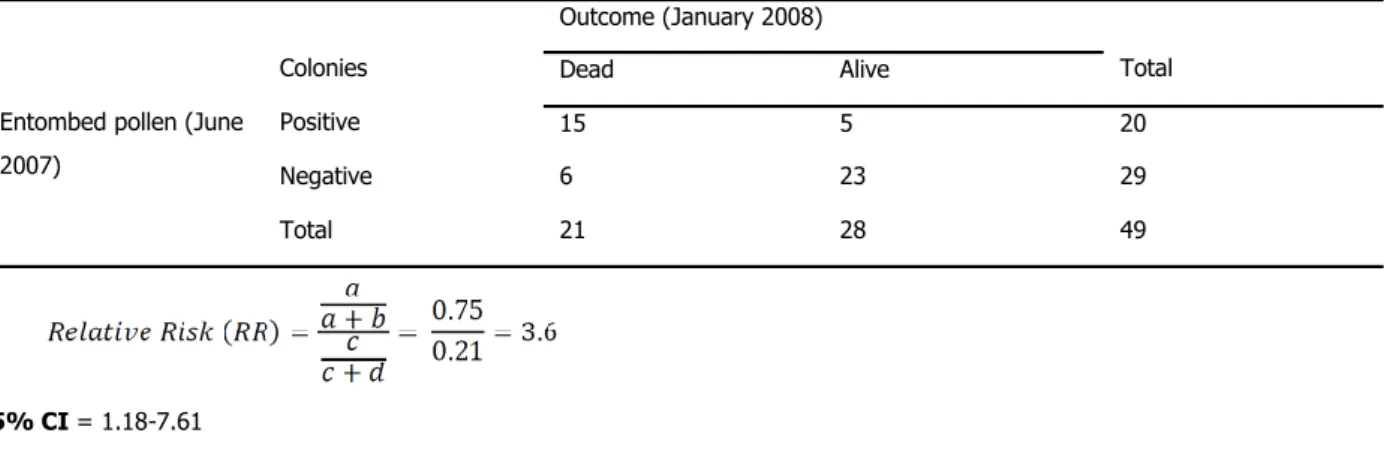
A longitudinal study was set up to monitor colonies for mortality and other factors as they moved up and down the east coast to pollinate crops. Forty nine colonies were examined in June of 2007, and 20 of them were found to have entombed pollen during the examination. In January 2008, 15 of the colonies that had entombed pollen were dead, as compared to the 6 colonies that died in the cohort without entombed pollen (vanEngelsdorp et al., 2009a).
95% CI = 1.18-7.61
As the RR is greater than 1 and the 95% CI do not overlap with 1, we can say that the increased risk of mortality associated with entombed pollen is significant. For every colony that died by January that did not have entombed pollen in June, 3.6 colonies died that did have entombed pollen.
Outcome (January 2008)
Colonies Dead Alive Total
Entombed pollen (June 2007)
Positive 15 5 20
Negative 6 23 29
Total 21 28 49
Outcome
Exposure Present Absent All Individuals
Yes A b a+b
No c d c+d
Table 3. Structure of data for calculation of Relative Risk. Both disease outcome and risk factor exposure are dichotomous.
exposure to the factor of interest is ascertained, for each case and control. Lastly, an odds ratio for the outcome of interest (in relation to exposure status) is calculated. Case-control studies are retrospective because they seek to determine previous exposure after the outcome has been established. Thus, they are subject to recall or information bias. Case-control studies are also subject to sampling bias because it is difficult to select controls which are (ideally) perfectly similar to cases, with the exception of outcome status. However, techniques such as matching controls to cases and stratified analysis can improve the precision of estimates from case-control studies.
Case-control studies are useful when attempting to isolate a cause or causes for an emerging disease condition. Most recently this approach was used in attempts to determine the factors contributing to Colony Collapse Disorder (CCD) (vanEngelsdorp et al., 2009b, 2010; Dainat et al., 2012)
2.1.3.1. Data analysis and interpretation
The data analysis is similar to that presented in cross-sectional study designs above. However, the results from case-control studies have more importance in determination etiology because exposure status is ascertained at a time prior to case and control status are determined.
2.2. Experimental study designs
In contrast to observational studies, an experimental study assigns subjects to different treatment or exposure levels. This type of study design can be used to investigate the change in health status due to disease screening programs, prevention plans, interventions, diagnostic techniques or treatment procedures. Ultimately, a research team decides who will be treated or exposed, which consequently results in experimental intervention, not just observation of natural events.
Randomized studies are very powerful for investigating cause and effect because of the random assignment of study subjects to two or more intervention strategies, which leads to a compelling test of causality. The most simple randomized trial design consists of participants being randomly assigned to one of two treatment arms, the experimental arm (receive treatment of interest) or the control arm (receive no, placebo or standard treatment). Data from randomized trials can be utilized to calculate incidence of outcomes per treatment arm and then compare the incidence using the relative risk or risk differences. Randomization helps protect against bias, because it is likely that potential confounders are equally distributed across the treatment and control study groups. The scope of randomized studies is limited because these studies aim to confirm or disprove a specific hypothesis. Additionally, the cost and time needed to conduct trials are two primary disadvantages of this study design. A third concern is that the results from a controlled randomized trial may not be generalizable to uncontrolled real-world settings. There are many different variations on the simple randomized study design in which randomization schemes are modified and researchers are blinded to study conditions.
3. Economic considerations
Understanding those factors that are associated with a lower rate of loss may provide potential treatment options for beekeepers. However, just because a practice appears to be effective in reducing loss does not mean that it is necessarily in the beekeeper’s best interest to adopt it. An additional piece of information for apiary managers is how much the treatment will cost and how much money the producer will likely save with its application.
Calculating the costs of practices in beekeeping is relatively straight forward, in that it includes the purchase cost of treatment and any labour or materials costs associated with its application. While each producer can calculate their costs, accurate aggregate data are more difficult to obtain, particularly for labour costs, or for
applications where producers use their own recipe. Thus, the true costs of treatment may vary from producer to producer, and individual managers can be guided to compare their own costs to the average for a better cost estimate.
Calculating the benefit from reducing disease is more nuanced. One simple approach is to use the replacement cost of a hive as an estimate for the benefit of losing one less colony. To be as close as possible to the actual cost, one would like to find the replacement process that most closely replicates the scenario of having not lost the colony in the first place, such as a nuclear colony. Thus, one would not simply want to use the cost of splitting a hive, but would want a replacement that would be as productive as quickly as an existing colony while not reducing the productivity of surviving colonies. The true replacement costs would include extra feeding and labour costs associated with getting that colony to productivity (Equations 3.0).
Equation 3.0.a
Benefit of saving one colony = Replacement cost
Where replacement cost = cost of nuclear colony + cost of feed + cost of labour
Once one has a measure of the benefit of saving one colony, one can determine the expected net benefit of treatment for a disease (Equation 3.0.b).
Equation 3.0.b
Expected net benefit of treatment =
Replacement cost x (mean survival of untreated colonies – mean survival of treated colonies)
Where: mean survival = 100 - Average Loss
If the cost of treatment exceeds the expected benefit, generating a negative expected net benefit, then despite the fact that the treatment may reduce colony loss, it may not be in the producer’s best interest to use that treatment.
Note that the above calculation, even if all treatment and replacement costs are included, will tend to underestimate the benefits associated with treatment. Disease not only affects mortality, it also affects productivity, which is not captured in the above calculation. Thus, the above calculation should be thought of as generating a lower bound on expected net benefit. A more nuanced approach would be to estimate the effect of treatment on disease load, and the effect of disease load on productivity of honey
production, pollination or other revenue-generating activities. Further, some beekeepers may place personal value on not losing a colony, and for them, their expected benefit of treatment may be higher still. These data are more difficult to collect, and will likely vary greatly from producer to producer. Nonetheless, giving beekeepers an estimate of the net benefit of treatment should allow them to compare the pure monetary costs and benefits to any other idiosyncratic costs of colony loss and help them in their management decisions.
4. Inferring causal relationships
using Hill’s Criteria
To diagnose the cause of a disease in honey bees, scientists typically compare observed symptoms with a list of exposures in colonies that implicate a particular pathogen, toxin or other detrimental aspect of the environment. Confirming the cause of the particular instance of these symptoms is relatively straightforward – the scientist either tests for the presence of the diagnosed causal agent itself or removes it and checks for amelioration of the symptoms. These approaches are feasible when the symptoms occur at the level of the individual or colony, because effects on growth, short-term survival or reproduction are readily measured (see the BEEBOOK paper on measuring colony strength parameters (Delaplane et al., 2013)). In principle, it is possible to estimate the impact of the disease on the population’s dynamics by using demographic models that quantify the effect on population growth (Varley et al., 1973).
There are some cases, however, that are problematic for two reasons. First, the symptom is itself a population-level attribute; for instance, a general population decline. Second, the normal procedure is reversed because the causal agent is already identified, albeit as a hypothesis. An example is the supposed role of trace dietary pesticides in causing honey bee declines. In this case, scientists are asked whether dietary exposure to the pesticide is capable of causing the observed population decline. Studying impacts at the population level by experiments with replicated comparisons presents a severe logistical challenge because the required manipulations are at the landscape scale. Some alternative tools are available, such as the classic ‘life table’ method of insect population ecology (Varley et al., 1973), but these can be applied only if detailed census data are
The COLOSS BEEBOOK: epidemiological methods 13
available that precisely identify causes of death over extended time periods. Where such resorts are stymied, scientists must use the available circumstantial evidence to pass an expert judgement. Hill’s criteria (Hill, 1965) provide a valuable framework that supports a repeatable and quantitative evaluation process.
Sir Austin Bradford Hill, a leading 20th century epidemiologist, identified nine types of information that provide ‘viewpoints’ from which to judge a proposed cause-effect relationship (Hill, 1965). The nine criteria include not only experimental evidence, but also eight kinds of circumstantial evidence that fall into two categories (Table 4).
For each criterion, scientists survey the available evidence and then formally describe the level of conviction with which they subsequently hold the proposed cause-effect hypothesis to be true: slight; reasonable; substantial; clear; and certain (Weiss, 2006). The descriptors are then associated with numerical values to produce a quantitative score of certainty (Cresswell et al., 2012). Specifically, an eleven-point scale for each criterion returns a positive value
(maximum five) if the evidence suggests that the agent certainly causes population decline, a negative value (maximum minus five) if the factor certainly does not and a zero if the evidence is equivocal or lacking. For example, if the evidence for a criterion gives a
reasonable indication that an agent does not cause the symptom, the score for that criterion would be -2, etc.
Box 8.
Using the numbers from the winter loss survey given in Box 6, we observed that beekeepers that used a known varroa mite control product lost 7.2% fewer colonies than beekeepers that did not use a product (29.5% versus 36.7% loss, respectively). To calculate the 95% CI for the difference in the mean, we need to calculate 1.96 × s.e.d, where s.e.d is the standard error of the difference in means. The standard error of the difference, s.e.d is defined as
where se1 is the standard error of the mean for sample 1, and s.e.2 is the standard error of the mean for sample 2. The standard error for the sample using treatment is 1.02 and the standard error for the control sample (or no-treatment sample) is 0.92. Thus, the standard error of the difference in means is
If using the replacement costs of a hive, including labour and feeding are $150, then the expected benefit of the treatment is the change in probability of loss times the replacement costs, or 0.07 × $150 = $10.80 (95% CI $8.07 to $13.53). Assume the cost of treatment is $7.50 per colony. Thus the expected net benefits would be $10.80 - $7.50 = $3.30 (95% CI $0.57 to $6.03) per hive. Thus, the producer is expected to benefit from the treatment and those benefits will range from $0.57 to $6.03, 95 times out of 100.
One major value of the criteria is that they disaggregate the different kinds of evidence, requiring the scientist to consider each kind carefully, separately and explicitly. Once the scores are given, there is no a priori reason either to give equal weight to the nine criteria or to calculate an average score. It is important, moreover, to consider whether any large scores have arisen principally on the theoretical criteria, because it is conventional in science to favour material evidence (i.e. associational criteria) over conjecture. For example, an evaluation by Hill’s criteria (Cresswell et al., 2012) revealed that the proposition that dietary pesticides cause honey bee declines was a substantially justified conjecture in the context of current knowledge (positive scores on the theoretical criteria), but was substantially contraindicated by a wide variety of circumstantial evidence (negative scores on the associational criteria). The disparity in the scores on the two categories of criteria explains in part the controversy over this question, because different constituencies make differential use of the two kinds of evidence. Hill (1965) himself refused to weight the criteria because the evaluation of circumstantial evidence cannot be made algorithmic.
The use of Hill’s criteria formalizes the evaluation of cause-consequence associations and applies a quantitative scoring method which makes the conclusions both apparent and repeatable. Since their inception over 40 years ago and subsequent widespread use, no criterion has been abandoned and none added, which means that they provide a stable and well-established infrastructure in which to process scientific evidence.
5. Conclusions
The general aim of all scientists studying honey bee health is the same; preservation of the bees. However, without common methods and shared terminology, it is difficult to confidently compare reported Table 4. The nine criteria established by Hill (1965), each with a brief description.
Criterion Brief description
1. Experimental evidence
2. Coherence Fails to contradict established knowledge 3. Plausibility Probable given established knowledge 4. Analogy Similar examples known
5. Temporality Cause precedes effect
6. Consistency Cause is widely associated with effect 7. Specificity Cause is uniquely associated with effect 8. Biological gradient Monotonic dose-response relationship 9. Strength Cause is associated with a substantive
effect
results. In an effort to standardize the efforts of those interested in improving honey bee health and make studies comparable, we have introduced epidemiological terminology, experimental design, and methods of calculation that are often different enough to preclude comparisons between studies.
6. References
ANDERSON, D (2013) Standard methods for Tropilaelaps mites research. In V Dietemann; J D Ellis; P Neumann (Eds) The COLOSS BEEBOOK, Volume II: standard methods for Apis mellifera pest and pathogen research. Journal of Apicultural Research 52(4): http://dx.doi.org/10.3896/IBRA.1.52.4.21 BREIMAN, I; FRIEDMAN, J H; OLSEN, R A; STONE, C J (1984)
Classification and regression trees. Wadsworth; Pacific Growe, CA, USA. 358 pp.
CRESSWELL, J E; DESNEUX, N; VANENGELSDORP, D (2012) Dietary traces of neonicotinoid pesticides as a cause of population declines in honey bees: an evaluation by Hill's epidemiological criteria. Pest Management Science: 68: 819-827.
http://dx.doi.org/10.1002/ps.3290
DAINAT, B; VANENGELSDORP, D; NEUMANN, P (2012) Colony Collapse Disorder in Europe. Environmental Microbiology Reports 4: 123-125. http://dx.doi.org/10.1111/j.1758-2229.2011.00312.x DE GRAAF, D C; ALIPPI, A M; ANTÚNEZ, K; ARONSTEIN, K A; BUDGE,
G; DE KOKER, D; DE SMET, L; DINGMAN, D W; EVANS, J D; FOSTER, L J; FÜNFHAUS, A; GARCIA-GONZALEZ, E; GREGORC, A; HUMAN, H; MURRAY, K D; NGUYEN, B K; POPPINGA, L; SPIVAK, M; VANENGELSDORP, D; WILKINS, S; GENERSCH, E (2013) Standard methods for American foulbrood research. In V Dietemann; J D Ellis; P Neumann (Eds) The COLOSS BEEBOOK, Volume II: standard methods for Apis mellifera pest and pathogen research. Journal of Apicultural Research 52(1):
http://dx.doi.org/10.3896/IBRA.1.52.1.11
DELAPLANE, K S; VAN DER STEEN, J; GUZMAN, E (2013) Standard methods for estimating strength parameters of Apis mellifera colonies. In V Dietemann; J D Ellis; P Neumann (Eds) The COLOSS BEEBOOK, Volume I: standard methods for Apis mellifera research. Journal of Apicultural Research 52(1):
http://dx.doi.org/10.3896/IBRA.1.52.1.03
ESTOUP, A; SOLIGNAC, M; CORNUET, J-M (1994) Precise assessment of the number of patrilines and of genetic relatedness in honey bee colonies. Proceedings of the Royal Society of London B, Biological Sciences 258: 1-7.
FOSGATE, G T (2009) Practical sample size calculations for surveillance and diagnostic investigations. Journal of Veterinary Diagnostic Investigation 21: 3-14.
GARDNER, M J; ALTMAN, D G (1986) Confidence intervals rather than P values: estimation rather than hypothesis testing. British Medical Journal 292: 746-750.
GENERSCH, E; VON DER OHE, W; KAATZ, H H; SCHROEDER, A; OTTEN, C; BERG, S; RITTER, W; GISDER, S; MEIXNER, M; LIEBIG, G; ROSENKRANZ, P (2010) The German bee monitoring project: a long term study to understand periodically high winter losses of honey bee colonies. Apidologie 41: 332-352.
http://dx.doi.org/10.1051/apido/2010014
GIRAY, T; GUZMAN NOVOA, E; ARON, C W; ZELINSKY, B; FAHRBACH, S E; ROBINSON, G E (2000) Genetic variation in worker temporal polyethism and colony defensiveness in the honey bee, Apis mellifera. Behavioural Ecology 11(1): 44-55. http://dx.doi.org/10.1093/beheco/11.1.44
GISDER, S; HEDTKE, K; MÖCKEL, N; FRIELITZ, M C; LINDE, A; GENERSCH, E (2010) Five-year cohort study of Nosema spp. in Germany: does climate shape virulence and assertiveness of Nosema ceranae? Applied and Environmental Microbiology 76: 3032-3038. http://dx.doi.org/10.1128/AEM.03097-09 HENDRIKX, P; CHAUZAT, M-P; DEBIN, M; NEUMAN, P; FRIES, I;
RITTER, W; BROWN, M; MUTINELLI, F; LE CONTE, Y; GREGORC, A (2009) Bee mortality and bee surveillance in Europe. Scientific report, European Food Safety Authority, Parma, Italy, pp. 217 (available at http://www.efsa.europa.eu/en/scdocs/doc/27e.pdf) HILL, A B (1965) The environment and disease: association or causation?
Proceedings of the Royal Society of Medicine 58: 295-300. HOLST, E C (1945) A simple field test for American foulbrood.
American Bee Journal 14: 34.
KOEPSELL, T D; WEISS, N S (2003) Epidemiologic methods: studying the occurrence of illness. Oxford University Press; New York, USA. MAUSNER, J S; KRAMER, S (1985) Epidemiology: an introductory text.
W B Saunders Company; Philadelphia, USA. 361
NUTTER, F W Jr (1999) Understanding the interrelationships between botanical, human, and veterinary epidemiology: the Ys and Rs of it all. Ecosystems Health 5: 131-140.
PAOLI, B; HAGGARD, L; SHAH, G (2002.) Confidence intervals in public health. Office of Public Health Assessment, Utah Department of Health, USA. p 8.
SAEGERMAN, C; SPEYBROECK, N; ROELS, S; VANOPDENBOSCH, E; THIRY, E; BERKVENS, D (2004) Decision support tools for clinical diagnosis of disease in cows with suspected bovine spongiform encephalopathy. Journal of Clinical Microbiology 42: 172-178. http://dx.doi.org/10.1128/JCM.42.1.172-178.2004
SAEGERMAN, C; PORTER, S R; HUMBLET, M F (2011) The use of modelling to evaluate and adapt strategies for animal disease control. Revue Scientifique et Technique - Office International des Épizooties 30: 555-569.
The COLOSS BEEBOOK: epidemiological methods 15
SPEYBROECK, N; BERKVENS, D; MFOUKOU-NTSAKALA, A; AERTS, M; HENS, N; HUYLENBROECK, G V; THYS, E (2004) Classification trees versus multinomial models in the analysis of urban farming systems in Central Africa. Agricultural Systems 80: 133-149. http://dx.doi.org/10.1016/j.agsy.2003.06.006
TOMA, B; BENET, J-J; DUFOUR, B; ELOIT, M; MOUTOU, F; SANAA, M (1991) Glossaire d'épidémiologie animale. Editions du Point Vétérinaire; Maisons-Alfort, France. 365 pp.
VANENGELSDORP, D; CARON, D; HAYES, J Jr; UNDERWOOD, R; HENSON, K R M; SPLEEN, A; ANDREE, M; SNYDER, R; LEE, K; ROCCASECCA, K; WILSON, M; WILKES, J; LENGERICH, E; PETTIS, J (2012) A national survey of managed honey bee 2010-11 winter colony losses in the USA: results from the Bee Informed Partnership. Journal of Apicultural Research 51: 115-124. http://dx.doi.org/10.3896/IBRA.1.51.1.14
VANENGELSDORP, D; EVANS, J D; SAEGERMAN, C; MULLIN, C; HAUBRUGE, E; NGUYEN, B K; FRAZIER, M; FRAZIER, J; COX-FOSTER, D; CHEN, Y; UNDERWOOD, R; TARPY, D R; PETTIS, J S (2009b) Colony Collapse Disorder: A descriptive study. PloS ONE 4: e6481. (available at:
http://www.plosone.org/article/info:doi/10.1371/journal.pone.0006481) VANENGELSDORP, D; EVANS, J D; DONOVALL, L; MULLIN, C;
FRAZIER, M; FRAZIER, J; TARPY, D R; HAYES, J Jr; PETTIS, J S (2009a). "Entombed Pollen": a new condition in honey bee colonies associated with increased risk of colony mortality. Journal of Invertebrate Pathology 101: 147-149.
http://dx.doi.org/10.1016/j.jip.2009.03.008
VANENGELSDORP, D; SPEYBROECK, N; EVANS, J D; NGUYEN, B K; MULLIN, C; FRAZIER, M; FRAZIER, J; COX-FOSTER, D; CHEN, Y; TARPY, D R; HAUBRUGE, E; PETTIS, J S; SAEGERMAN, C (2010) Weighing risk factors associated with bee Colony Collapse Disorder by classification and regression tree analysis. Journal of Economic Entomology 103: 1517-1523. (available at:
http://www.bioone.org/doi/pdf/10.1603/EC09429)
VANENGELSDORP, D; BRODSCHNEIDER, R; BROSTAUX, Y; VAN DER ZEE, R; PISA, L; UNDERWOOD, R; LENGERICH, E J; SPLEEN, A; NEUMANN, P; WILKINS, S; BUDGE, G E; PIETRAVALLE, S; ALLIER, F; VALLON, J; HUMAN, H; MUZ, M; LE CONTE, Y; CARON, D; BAYLIS, K; HAUBRUGE, E; PERNAL, S;
MELATHOPOULOS, A; SAEGERMAN, C; PETTIS, J S; NGUYEN, B K (2011) Calculating and reporting managed honey bee colony losses. In D Sammataro; J A Yoder (Eds). Honey bee colony health: challenges and sustainable solutions. CRC Press; FL, USA. pp. 237-244
VANENGELSDORP, D; SAEGERMAN, C; NGUYEN, K B; PETTIS J S (2013) Honey bee health surveillance. In W Ritter (Ed.). OIE Technical Series no 12: The vet and the bee. OIE. (in press).
VANENGELSDORP, D; TARPY, D R; LENGERICH, E J; PETTIS, J S (2013) Idiopathic brood disease syndrome and queen events as precursors of colony mortality in migratory beekeeping operations in the eastern United States. Preventive Veterinary Medicine. (in press). VARLEY, G C; GRADWELL, G R; HASSELL, M P (1973) Insect
population ecology. Blackwell Scientific Publications; Oxford, UK.
WEISS, N S (2006) Clinical epidemiology: the study of the outcome of illness (Third edition). Oxford University Press; UK. 178 pp WORLD HEALTH ORGANISATION (WHO) (1999) Norms and standards
in epidemiology: case definitions. Epidemiological Bulletin 20. WOODWARD, M (2005) Epidemiology. Study design and data