arXiv:1506.08572v1 [astro-ph.SR] 29 Jun 2015
The changing UV and X-ray properties of the Of?p star
CPD −28
◦
2561
⋆
Ya¨el Naz´e
1†‡
, Jon O. Sundqvist
2,3, Alex W. Fullerton
4, Asif ud-Doula
5, Gregg A. Wade
6,
Gregor Rauw
1, Nolan R. Walborn
41GAPHE, Universit´e de Li`ege, Quartier Agora, All´ee du 6 Aoˆut 19c, Bat. B5C, B4000-Li`ege, Belgium 2University of Delaware, Bartol Research Institute, Newark, Delaware 19716, USA
3Institut f¨ur Astronomie und Astrophysik der Universit¨at M¨unchen, Scheinerstr. 1, 81679 M¨unchen, Germany 4Space Telescope Science Institute, 3700 San Martin Drive, Baltimore, MD 21218, USA
5Penn State Worthington Scranton, Dunmore, PA 18512, USA
6Department of Physics, Royal Military College of Canada, PO Box 17000, Station Forces, Kingston, ON K7K 4B4, Canada
ABSTRACT
The Of?p star CPD −28◦2561 was monitored at high energies with XMM-Newton and HST. In X-rays, this magnetic oblique rotator displays bright and hard emission that varies by ∼55% with rotational phase. These changes occur in phase with optical variations, as expected for magnetically confined winds; there are two maxima and two minima in X-rays during the 73d rotational period of CPD −28◦2561. However, contrary to previously studied cases, no
signif-icant hardness variation is detected between minima and maxima, with the exception of the second minimum which is slightly distinct from the first one. In the UV domain, broad-band fluxes remain stable while line profiles display large variations. Stronger absorptions at low velocities are observed when the magnetic equator is seen edge-on, which can be reproduced by a detailed 3D model. However, a difference in absorption at high velocities in the C iv and N v lines is also detected for the two phases where the confined wind is seen nearly pole-on. This suggests the presence of strong asymmetries about the magnetic equator, mostly in the free-flowing wind (rather than in the confined dynamical magnetosphere).
Key words: Stars: individual: CPD −28◦2561– Stars: early-type – Stars: magnetic field – Stars: mass-loss – X-rays: stars – Ultraviolet: stars
1 INTRODUCTION
The massive O-type star CPD −28◦2561 has been known to be
pe-culiar for forty years, as it showed a He ii λ4686 line too strong in comparison to the neighbouring N iii emission lines, broad He ii lines but sharp He i lines, and strong carbon lines but weak ni-trogen lines (Walborn 1973; Garrison et al. 1977). However, the causes underlying its strangeness remained hidden until its thor-ough investigation began, only a few years ago, in the framework of the O and WN survey (Barb´a et al. 2010, 2014). At the time, the peculiarities of CPD −28◦2561 were found to be similar to
those of other members of the class of Of?p stars, despite the ab-sence of strong C iii λ 4650 lines (the initial defining characteristic
⋆ Based on observations made with XMM-Newton (ObsID # 074018) and and HST (program # 13629). XMM-Newton is an ESA Science Mission with instruments and contributions directly funded by ESA Member states and the USA (NASA). The NASA/ESA Hubble Space Telescope is operated by the Association of Universities for Research in Astronomy, Inc., under NASA contract NAS 5-26555.
† Research Associate FRS-FNRS
‡ E-mail: naze@astro.ulg.ac.be
of the Of?p class, see Walborn 1972; Naz´e et al. 2008b for more details). It thus became one of the five known Galactic Of?p stars (Walborn et al. 2010).
Since 2001, it has become clear that the Of?p category gath-ers massive stars exhibiting several interesting properties. To the presence of peculiar lines or line profiles (e.g. strong C iii λ 4650 emission, narrow emissions in Balmer lines, UV line profiles dif-ferent from those of supergiant Of stars) in their spectra was thus added the presence of periodic variability, notably of their Balmer and He i lines in the optical domain (e.g. Naz´e et al. 2001; Walborn et al. 2004), but also of their overall brightness (e.g. Barannikov 2007) and of their (unusually bright) X-ray emission (e.g. Naz´e et al. 2004; Naz´e et al. 2007; Naz´e et al. 2008a). The recurrence timescales range from 7d up to several decades (e.g. Walborn et al. 2004; Naz´e et al. 2006; Naz´e et al. 2008a). More-over, and most importantly, strong magnetic fields with global dipo-lar topologies (e.g. Donati et al. 2006; Martins et al. 2010) were also found to be present in all Galactic Of?p stars.
These characteristics are understood within the framework of magnetic oblique rotators. For massive stars, a strong magnetic field is able to channel the stellar wind outflow. The effectiveness of
the process can be characterized by the wind-confinement param-eter (ud-Doula & Owocki 2002), defined as η∗ ≡B2dR
2
∗/( ˙MB=0v∞),
with R∗ the stellar radius, v∞the wind terminal velocity, Bd the
dipole equatorial surface field strength, and ˙MB=0 the mass-loss
rate the star would have if it had no magnetic field1. The Alfv´en
radius, at which the magnetic and wind energy densities are equal, is RA ≈η1/4∗ R∗and it is located above the stellar surface if η∗ >1.
Below the Alfv´en radius, the magnetic field is strong enough to channel the radiatively driven wind outflow along closed field lines. The trapped wind plasma channelled along field lines from oppo-site poles then collides at the magnetic equator. As a result, there is an overdense region around the magnetic equator, which is seen under different angles and/or with different degrees of occultation as the star rotates, explaining the recurrent changes seen throughout the electromagnetic spectrum (for an example of modelling optical variations in this framework, see Sundqvist et al. 2012).
Since massive O stars have high mass-loss rates, the presence of a strong magnetic field has another consequence for those stars: a rapid spindown due to magnetic braking (ud-Doula et al. 2009), which explains why the Of?p stars rotate slowly. In such a case, ro-tation is dynamically unimportant and the confined wind plasma falls back to the star by gravity, generating a “dynamical mag-netosphere” around the star (e.g. Petit et al. 2013, and references therein).
Indeed, this is the case of CPD −28◦2561, for which a
strong magnetic field was initially detected by Hubrig et al. (2011, 2012). Subsequent spectroscopic and spectropolarimetric monitor-ing (Wade et al. 2015) further established the star’s properties: its (rotation) period is 73.41d, its surface dipolar field Bd amounts
to ∼2.5 kG, and its wind magnetic confinement parameter η∗ is
about 100, implying strong confinement. Notably, during one mag-netic cycle, the Balmer and He i lines present a double-wave vari-ation, i.e. their emission component is maximum (resp. minimum) twice per period, at φ = 0.0 and 0.5 (resp. 0.25 and 0.75). In the framework of magnetic oblique rotators, such an observation im-plies that both magnetic poles are seen during the stellar rotation, as for the magnetic O9.2 IV star HD 57682 (Grunhut et al. 2012), implying that the sum of the inclination i and the magnetic obliq-uity β angles is large. Indeed, Wade et al. (2015) derived (i, β) or (β, i) = (90◦,35◦). With such a configuration, MHD modelling is
able to reproduce the variations of the equivalent width of the Hα line (Wade et al. 2015).
Continuing the work of Wade et al. (2015), we present in this paper high-energy monitoring of CPD −28◦2561, using
XMM-Newton and HST data. Section 2 presents the observations while
the two following sections provide the observational and modelling results in the X-ray and UV domains, respectively. Finally, a sum-mary and conclusions are given in Section 5.
1 This is essentially the mass feeding rate from the photosphere into the magnetic wind (see e.g. Table 4). It is important to realize here that this ˙MB=0 is not the actual mass-loss rate of the star; this actual mass
loss is significantly reduced (of the order of ∼ 80 % for η∗ ≈ 60, cf. ud-Doula, Owocki & Townsend 2008) due to the trapped plasma that even-tually falls back onto the star.
magnetic axis
magnetosphere
dynamical magnetic equator
φ=0.11 φ φ=0.02 φ=0.46 =0.24 =0.74 R RA *
open field lines
closed field lines
Figure 1. Schematic diagram of the system, showing the orientation of the
magnetically confined winds of CPD −28◦2561 with respect to the observer at the phases of the five XMM-Newton observations. Note that the three HST observations were obtained simultaneously with XMM, at φ = 0.01, 0.25, and 0.49.
2 OBSERVATIONS 2.1 X-ray data
In 2014, XMM-Newton (Jansen et al. 2001) observed
CPD −28◦2561 five times, for 10–20 ks each time to monitor
the changes of the X-ray emission with phase (PI Naz´e). Table 1 lists the observation identifiers, the dates, the actual durations (all well below one hundredth in phase), and the phases of the exposures, derived using the ephemeris of Wade et al. (2015,
T0=2 454 645.49 and P=73.41 d). Note that the first four
observa-tions were obtained within the same cycle, but the last one could only be scheduled six months later: this has however not much impact on the phase, considering the small uncertainties on the ephemeris (Wade et al. 2015). The five exposures sample the two maxima, the two minima, and one intermediate phase in the star rotational cycle (see Fig. 1 for the orientation of the system at these phases).
The XMM-Newton data were reduced with the standard Sci-ence Analysis System (SAS) software v14.0.0 using calibration files available in December 2014 and following the recommenda-tions of the XMM-Newton team2. Only the best-quality EPIC data
(Str¨uder et al. 2001; Turner et al. 2001) were kept (PAT T ERN of 0–12 for MOS and 0–4 for pn, note that the source is too faint to have usable RGS data). Large background flares were observed in two exposures (ObsID 0740180501 and 0740180701). The analy-sis was performed with the times of these flares either retained or discarded. As both analyses yielded similar results, we show below only the results for the cleaned datasets.
2 SAS threads, see
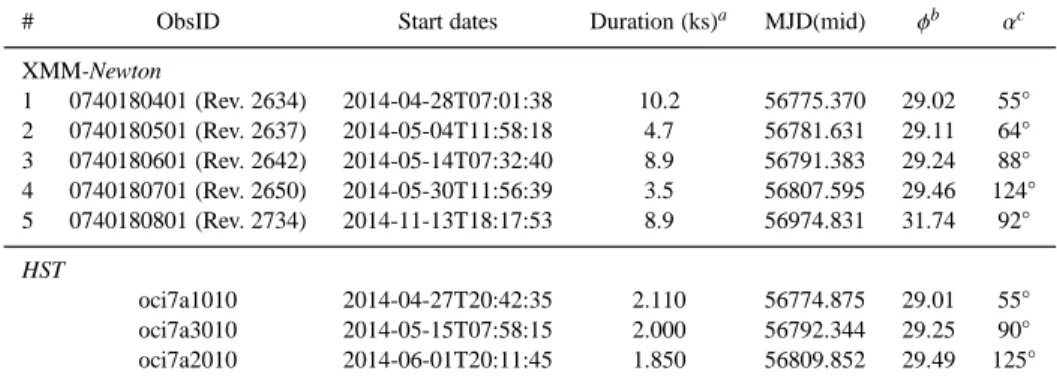
Table 1. Journal of observations.
# ObsID Start dates Duration (ks)a MJD(mid) φb αc
XMM-Newton 1 0740180401 (Rev. 2634) 2014-04-28T07:01:38 10.2 56775.370 29.02 55◦ 2 0740180501 (Rev. 2637) 2014-05-04T11:58:18 4.7 56781.631 29.11 64◦ 3 0740180601 (Rev. 2642) 2014-05-14T07:32:40 8.9 56791.383 29.24 88◦ 4 0740180701 (Rev. 2650) 2014-05-30T11:56:39 3.5 56807.595 29.46 124◦ 5 0740180801 (Rev. 2734) 2014-11-13T18:17:53 8.9 56974.831 31.74 92◦ HST oci7a1010 2014-04-27T20:42:35 2.110 56774.875 29.01 55◦ oci7a3010 2014-05-15T07:58:15 2.000 56792.344 29.25 90◦ oci7a2010 2014-06-01T20:11:45 1.850 56809.852 29.49 125◦
Notes:afor XMM-Newton, this corresponds to the on-axis actual (i.e., after discarding flares) duration for the pn camera;bPhases at mid-exposure using the
ephemeris of Wade et al. (2015);cAngle between the magnetic axis and the line-of-sight, which can be calculated using cos α = sin β cos(2πφ) sin i + cos β cos i.
To extract spectra and lightcurves, we must first derive the best source position. To this end, we applied a source detection algo-rithm on each exposure using the task edetect chain and a likeli-hood of 10. This was done in the 0.4–10.0 keV range, considering two energy bands (a soft band corresponding to the 0.4–2.0 keV energy band and a hard band to the 2.0–10.0 keV band). This de-tection run provided the count rate of CPD −28◦2561 for each
ob-servation (Table 2) in addition to best-fit positions. To get spectra using the task especget, source events were then extracted in circu-lar regions centered on these best-fit positions and with a radius of 38′′ (except for the last exposure, where it was reduced to 33′′to
avoid CCD gaps). Background events were extracted in a circular region with a radius of 45′′(except for the pn data in the last
expo-sure, where it was reduced to 33′′) and centered as close as
possi-ble to the target considering crowding and CCD edges. The relative position of background and source was kept the same throughout exposures and cameras (except for the pn data in the last expo-sure). The EPIC spectra were grouped, using specgroup, to obtain an oversampling factor of five and to ensure that a minimum signal-to-noise ratio of three (i.e. a minimum of 10 counts) was reached in each spectral bin of the background-corrected spectra. After ap-plying the barycentric correction to event files, EPIC lightcurves were produced for the same regions in the 0.4-2.0 keV (soft), 2.0-10.0 keV (hard), and 0.4-2.0-10.0 keV (total) bands and with 1ks time bins. They were then corrected using epiclccorr to get equivalent on-axis, full PSF count rates corrected for (known) photon losses. In addition, as previous experience shows, very large errors and wrong estimates of the count rates are avoided by discarding bins displaying effective exposure time <50% of the time bin length. We also checked that the raw source+background lightcurves and the background-corrected lightcurves of the source yield similar re-sults. Finally, it may be noted that the source is not bright enough to present pile-up.
2.2 UV data
2.2.1 Photometry
In parallel to its X-ray telescopes, XMM-Newton possesses a small optical/UV telescope called the Optical Monitor (OM, Mason et al. 2001) which aims at observing faint sources. With the OM, we ob-tained UV photometry of CPD −28◦2561 in both the UVM2 filter
(centered on 2310Å with a width of 480Å) and the UVW2 filter (centered on 2120Å with a width of 500Å). For each filter, five
short subexposures of 1–2ks were taken, except for the third
XMM-Newton observation where only one long exposure of 5ks was
ob-tained per filter. The data were acquired in image mode for all ex-posures except the last one (which used only one filter, UVM2, and the image-fast mode). No photometry in other filters could be ob-tained as CPD −28◦2561 is too bright in the other bands. In fact, the
target is so bright (about 400 counts per seconds in the UVM2 filter and 200 cts s−1 in the UVW2 filter) that coincidence loss
correction may introduce errors in the results (particularly in fast mode) -see section 4.1 for details. As recommended by the SAS team, we reduced these data using the task omichain and omfchain (the lat-ter for the fast mode only). Note that CPD −28◦2561 has no close
neighbour nor any close straylight feature which could contaminate its photometry.
2.2.2 Spectroscopy
In addition to the XMM-Newton data, we also obtained three ultra-violet spectra of CPD −28◦2561 with the Space Telescope
Imag-ing Spectrograph (STIS) on board the Hubble Space Telescope (HST) under the auspices of the Joint HST/XMM-Newton Observ-ing Proposals program. Table 1 provides a journal of these observa-tions, which constitute HST GO Program 13629 (PI: Naz´e). They were obtained nearly simultaneously with the first, third, and fourth XMM-Newton observations, i.e. they sample the two maxima and one minima according to the ephemeris of Wade et al. (2015).
All the STIS spectra were obtained in the same manner. The observing sequence consisted of a standard spectroscopic acqui-sition in the F28X50OII aperture, an “auto-wavecal” exposure of the internal Pt-Cr/Ne wavelength calibration lamp, and a single ex-posure of CPD −28◦2561 through the 0.2′′ ×0.2′′ aperture with
the standard ACCUM mode of the far-ultraviolet MAMA photon-counting detector. Spectra were produced by the E140M grating, which provided wavelength coverage from 1144 Å (order 129) to 1729 Å (order 86) with a resolving power of ∼46 000. Since suc-cessive visits had a decreasing visibility window, the exposure time varied from 2.11 to 1.85 ks, but in all cases produced a signal-to-noise ratio of about 30 per pixel near the blaze maximum of the most sensitive orders.
The spectra were uniformly processed with version 3.3 (2013 October 03) of the CALSTIS pipeline, which included correction for detector nonlinearity, dark current subtraction, flat field cor-rection, determination and application of corrections to the
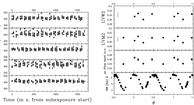
wave-Figure 2. Intra-pointing lightcurves derived from the XMM-Newton observations. The x-axis gives the time, in seconds, elapsed since the beginning of the
observation. Black dots correspond to pn data, green triangles to MOS1 data, and red crosses to MOS2 data. Each row corresponds to one observation and displays the lightcurves in three different bands (from left to right: total, soft, hard).
length zero point, 1-D spectral extraction of each order, application of dispersion solutions, photometric calibration, and scattered-light corrections. Additional effort was devoted to extracting order 86, which contains the N iv λ 1718 resonance line. Although this order falls completely on the MAMA detector and is well separated from adjacent orders, it has not been routinely extracted by CALSTIS for the past few observing cycles. This exclusion is evidently due to small shifts in the location of the order, which push the regions used to model the background and scattered light off the detector and preclude the standard correction for these effects. Since these corrections are less significant for orders that are well-separated, we developed a simplified method of tracing the order, estimating the local background, and extracting the net count rates that uses modified versions of the current reference files.
As a final step, the extracted, calibrated orders for each obser-vation were merged into a single spectrum.
3 THE X-RAY EMISSION OF CPD −28◦2561
In strongly magnetic massive stars, the collision between the wind flows from both hemispheres produces a bright and hard X-ray emission (Babel & Montmerle 1997a; ud-Doula et al. 2014, and references therein). Depending on the geometry of the magneto-sphere, the X-ray emitting regions in such a magnetic oblique ro-tator may be regularly occulted by the star as the system rotates, which yields periodic X-ray variations locked in phase with other periodically variable quantities, such as the recorded magnetic field and the intensities of optical lines. In the next subsections, we ex-amine the properties of the X-ray emission of CPD −28◦2561, to
determine its intensity, variability, and relationship to other obser-vational quantities. -0.5 0 0.5 1 1.5 0 0.02 0.04 0.06 0 0.005 0.01 0.015 0.02 -0.8 -0.6 -0.4 -0.2 -0.5 0 0.5 1 1.5 2 0 -2
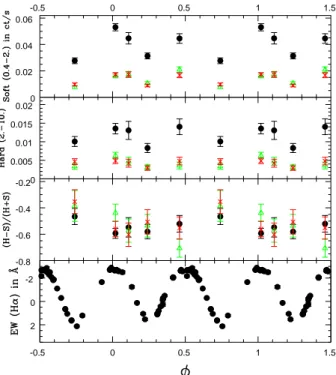
Figure 3. Evolution with phase of the X-ray count rates in the different
bands and of the X-ray hardness ratio of CPD −28◦2561, compared to the Hα variations recorded in the optical domain (Wade et al. 2015). Black dots correspond to pn data, green triangles to MOS1 data, and red crosses to MOS2 data.
3.1 Lightcurves
We searched for X-ray variability in the light curves of CPD −28◦2561 that occurs on short (intra-pointing) and long
we applied a series of χ2 tests (with three different null
hypothe-ses: constancy, linear variation, quadratic variation, as for ζ Pup, Naz´e et al. 2013) to the derived lightcurves (Fig. 2). We further compared the improvement of the χ2 when increasing the
num-ber of parameters in the model (e.g. linear trend vs constancy) by means of F-tests. Adopting a significance level (SL) of 1%, we found that the lightcurves are never significantly variable, but also that the pn lightcurves in the total and soft bands of the first, third, and last exposures are significantly better fit by linear or parabolic trends than by a constant. Indeed, these lightcurves (left panels of Figure 2) show obvious maxima with flux dropping on each side or minima with flux increasing on each side. The larger noise in MOS data (due to redirection of half of their flux into the RGS) prevents us from confirming these results. While more precise X-ray data are needed for a more complete investigation, the detected variations can already be easily understood qualitatively. In fact, the short-term variability only reflects the phase-locked variations of the star with the rotational period. As we will see below, X-ray and optical emissions vary simultaneously: as the phases of these observations correspond to extrema in the optical spectrum and X-ray emission, this explains the shape of the observed lightcurves (which are simply close-up on maxima or minima).
The similarity in behaviour between X-ray and optical do-mains is evident from the analysis of the inter-pointing variability. When phased with the ephemeris of Wade et al. (2015, see Table 2 and Fig. 3), the count rates derived from the source detection algo-rithm show maxima at φ = 0.0 and 0.5, and minima at φ = 0.25 and 0.75, with the intermediate phase (φ = 0.11) yielding inter-mediate results. It may be noted that the total and soft count rates of the second maximum (φ ∼ 0.5) are slightly smaller than those of the first one (φ ∼ 0), but this difference is small (less than 3σ, see Table 2). As for θ1Ori C (Gagn´e et al. 2005; Stelzer et al. 2005)
and HD 191612 (Naz´e et al. 2007, 2010), the X-ray flux variations are thus clearly phased with the stellar rotation period, as demon-strated by the simultaneous minima in X-ray and optical emissions (Fig. 3). In addition, the amplitude of the X-ray changes is also similar: the maximal count rates of CPD −28◦2561 are ∼60% larger
than the minimal ones, comparable to what is observed for θ1Ori C,
HD 191612, and Tr16-22 (Naz´e et al. 2014a).
In addition to brightness changes, varying spectral shapes are observed for the X-ray emission of θ1Ori C, HD 191612, and
Tr16-22 (Naz´e et al. 2014a). The presence of such X-ray hard-ness changes is probably related to a temperature stratification in the magnetospheric plasma, with the warm and hot regions be-ing occulted by different amounts. The situation appears different for CPD −28◦2561, however, as no significant variations of
hard-ness are present over the first four exposures and only a slightly harder emission is found in the last observation. The stratification in the magnetosphere of CPD −28◦2561 thus appears less pronounced
than in other magnetic O-stars.
The variations in X-ray brightness are generally considered to be mostly due to occultation of the X-ray emitting regions by the stellar body as the star rotates. To test to what extent such an occultation can account for X-ray variation in CPD −28◦2561, we
employed a simple toy model wherein the X-ray emission region is an optically-thin ring-like region in the magnetic equatorial plane with negligible thickness but varying widths. One can then derive the expected degree of occultation as a function of geometry of the region, phase, inclination of the star (i), and magnetic obliquity (β). We tested different geometries: a “disk” from R∗to RAand a ring
with a radius restricted to R = (RA−R∗/2) ± R∗/2, which better
mimics the X-ray emitting regions seen in MHD simulations (e.g.
ud-Doula, Owocki & Townsend 2008). We also tested several pos-sibilities for the brightness distribution within the X-ray emitting region: uniform brightness, brightness varying as r−2, and
bright-ness varying as r−4. For the parameters (i, β, R
A) of the three
mag-netic stars with known geometry and X-ray monitoring (θ1Ori C,
HD 191612, and CPD −28◦2561), the ratio between the maximum
and minimum fluxes predicted by this simple model amounts to 110%–130%, and it does not change when considering thicker ring-like regions. This predicted ratio is smaller than the observed ratios (∼140–160%), suggesting that the simple occultation of optically-thin regions near RA is not the dominant process at the origin of
the X-ray variations. However, if such emitting regions are located closer to the photosphere, the agreement is better. But it is not obvi-ous how X-rays could be produced near the surface as this process requires high wind shock velocities which can only occur further out. Clearly, a more sophisticated modelling is required, and will be investigated in the future using fully self-consistent 3D MHD models.
3.2 Spectra
To get more detailed information, we then turned to the X-ray spectra (Fig. 4). The five observations were considered separately, as variations exist (see previous section), but the fitting proce-dure was kept the same. For each observation, all EPIC data (MOS1, MOS2, and pn) were fitted simultaneously within Xspec v12.8.2 using absorbed optically-thin thermal plasma models, i.e.
wabs × phabs ×Papec, with solar abundances (Asplund et al.
2009). The first absorption component is the interstellar column, fixed to 1.8 × 1021cm−2 (a value calculated using the conversion
formula 5.8 × 10²¹×E(B − V) cm−2from Bohlin et al. 1978 and the
color excess of the star E(B−V)=0.31, estimated from B−V=0.04), while the second absorption represents additional (local) absorp-tion. For the emission component, we proceeded in several steps. First, we considered two thermal components (one thermal compo-nent was not enough to achieve a good fitting). In the resulting fits, the additional absorption and temperatures did not significantly dif-fer amongst datasets. We then fixed them to 3.8×1021cm−2, 0.8 keV
and 3.0 keV, respectively, for a last set of fits. Second, to reproduce (to first order) a multi-temperature plasma, we fitted a series of four emission components with temperatures fixed to 0.2, 0.6, 1.0, and 4.0 keV as used in the global X-ray analysis of magnetic hot stars by Naz´e et al. (2014a). This allows us to directly compare with the global survey results. In these fits, the additional absorption was not observed to significantly vary, hence we decided to fix it at the average value of 6.6 × 1021cm−2for another set of fits. Spectral
pa-rameters derived by these different fitting procedures are provided in Table 3 (see also Fig. 5). It should be noted that the different types of models yield similar χ2and similar results, within the
er-rors.
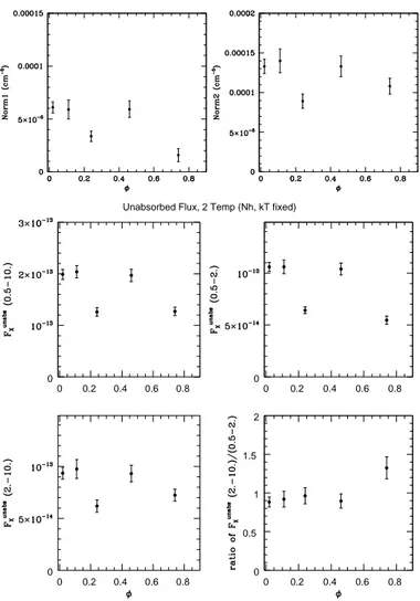
The fitting results agree with what was derived from the count rates: the ISM-absorption corrected fluxes appear larger by ∼55% at maxima (φ = 0.02, 0.11, and 0.46) compared to minima (φ = 0.24 and 0.74), while the hardness of the X-ray emission (traced by the flux ratio and the relative importance of normalization fac-tors, or average temperature3) increases only in the last observation
(φ = 0.74). While the two maxima are quite similar, it clearly ap-pears that the two minima (at phases 0.24 and 0.74) are different
3 Note however that the average temperature is not always a consistent es-timate of plasma hardness (Naz´e et al. 2014a).
Table 2. X-ray photometry of CPD −28◦2561. The hardness ratio is defined as HR = (H − S )/(H + S ), with S and H the count rates in the soft (0.4–2.0 keV) and hard (2.0–10.0 keV) bands, respectively.
# φ pn (cts s−1) MOS1 (cts s−1) MOS2 (cts s−1)
Total Soft Hard HR Total HR Total HR
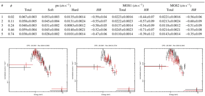
1 0.02 0.067±0.003 0.053±0.003 0.0135±0.0014 −0.59±0.04 0.0223±0.0016 −0.44±0.07 0.0221±0.0016 −0.56±0.06 2 0.11 0.058±0.005 0.045±0.004 0.0131±0.0024 −0.55±0.07 0.0222±0.0023 −0.57±0.09 0.0213±0.0024 −0.60±0.09 3 0.24 0.040±0.003 0.031±0.002 0.0083±0.0012 −0.58±0.05 0.0137±0.0014 −0.54±0.09 0.0118±0.0012 −0.51±0.09 4 0.46 0.059±0.004 0.045±0.004 0.0140±0.0021 −0.52±0.06 0.0245±0.0023 −0.71±0.07 0.0214±0.0021 −0.55±0.08 5 0.74 0.038±0.003 0.028±0.002 0.0101±0.0014 −0.47±0.06 0.0110±0.0014 −0.39±0.12 0.0143±0.0014 −0.35±0.09 1 10 10 −3 0.01 normalized counts s −1 keV −1 Energy (keV) CPD −28 2561 : Rev 2634 & 2650 1 10 10 −3 0.01 normalized counts s −1 keV −1 Energy (keV) CPD −28 2561 : Rev 2642 & 2734 1 10 10 −3 0.01 normalized counts s −1 keV −1 Energy (keV) CPD −28 2561 : Rev 2634 & 2642
Figure 4. X-ray spectra of CPD −28◦2561 in the XMM-Newton observations. Only pn data are shown for clarity. Left: Comparison between the pn data taken at the two maxima (φ = 0.02 in black, φ = 0.46 in red). Middle: Comparison between the pn data taken at the two minima (φ = 0.24 in black, φ = 0.74 in red). Right: Comparison between the pn data taken at the first maximum (φ = 0.02 in black) and the first minimum (φ = 0.24 in red).
Table 3. Best-fit parameters for the fit of X-ray (EPIC) spectra. model with 2 thermal components
# φ NH kT1 norm1 kT2 norm2 χ2(dof) FXobs(tot.) (soft) (hard) FXunabs
(1022cm−2) (keV) (10−5cm−5) (keV) (10−4cm−5) (10−14erg cm−2s−1)
1 0.02 0.34±0.29 0.76±0.12 5.16±6.76 2.71±0.39 1.40±0.14 0.96(77) 16.2±1.4 7.45±0.60 8.70±0.91 19.6 2 0.11 0.35±0.25 0.86±0.12 5.08±5.52 2.71±0.71 1.42±0.23 0.93(33) 16.4±2.6 7.46±1.00 8.92±1.90 19.7 3 0.24 0.26±0.26 0.96±0.18 2.55±2.54 3.08±0.98 0.84±0.13 1.05(40) 10.5±1.0 4.50±0.41 5.97±1.30 12.5 4 0.46 0.66±0.34 0.58±0.35 17.3±194. 3.85±4.21 1.20±0.62 1.17(42) 17.4±3.3 7.50±0.90 9.94±2.64 20.8 5 0.74 0.31±0.35 1.03±0.40 1.86±3.27 3.94±2.47 0.96±0.23 1.29(32) 12.1±2.2 3.95±0.75 8.17±1.80 13.7 1 0.02 0.38f 0.8f 6.10±0.52 3.f 1.33±0.09 0.95(80) 16.6±0.8 7.39±0.30 9.18±0.56 19.9 2 0.11 0.38f 0.8f 5.90±0.90 3.f 1.40±0.15 0.88(36) 17.0±1.0 7.45±0.46 9.56±0.88 20.4 3 0.24 0.38f 0.8f 3.37±0.50 3.f 0.89±0.09 1.02(43) 10.6±0.7 4.52±0.23 6.07±0.58 12.6 4 0.46 0.38f 0.8f 5.93±0.78 3.f 1.33±0.13 1.16(45) 16.4±1.0 7.28±0.40 9.15±0.78 19.7 5 0.74 0.38f 0.8f 1.58±0.61 3.f 1.08±0.10 1.22(35) 11.0±0.7 3.98±0.28 7.11±0.57 12.7
model with 4 thermal components of temperatures 0.2, 0.6, 1.0, and 4.0 keV
# φ NH norm1 norm2 norm3 norm4 χ2(dof) FXobs(tot.) (soft) (hard) FXunabs
(1022cm−2) (10−4cm−5) (10−5cm−5) (10−5cm−5) (10−4cm−5) (10−14erg cm−2s−1) 1 0.02 0.86±0.17 9.88±9.70 8.16±6.36 7.48±3.61 9.96±1.30 0.94(77) 16.9±1.0 7.62±0.50 9.27±0.85 20.5 2 0.11 0.76±0.22 7.25±10.4 0.±5.05 11.6±5.60 10.1±2.10 0.96(33) 17.2±5.5 7.51±4.70 9.74±1.90 20.8 3 0.24 0.50±0.20 0.98±17.2 0.±2.40 4.85±1.72 7.20±1.42 1.07(40) 11.1±2.1 4.51±1.48 6.59±0.90 13.2 4 0.46 0.83±0.36 7.56±22.5 16.0±10.3 1.00±5.39 11.7±1.80 1.15(42) 17.6±3.0 7.54±2.80 10.1±1.50 21.1 5 0.74 0.34±0.43 0.0(unconstrained) 0.±6.30 2.01±2.87 9.63±1.23 1.26(33) 12.2±1.3 3.95±0.90 8.25±0.75 13.8 1 0.02 0.66f 3.71±1.96 6.24±3.63 6.14±1.99 10.6±1.10 0.95(78) 17.2±1.0 7.54±0.28 9.69±0.79 20.9 2 0.11 0.66f 4.44±2.53 0.±4.77 10.5±2.80 10.4±1.80 0.94(34) 17.4±3.2 7.48±1.43 9.88±1.26 20.9 3 0.24 0.66f 2.32±1.69 0.03±2.96 6.29±1.58 6.77±1.16 1.05(41) 10.9±2.1 4.53±1.44 6.38±0.85 13.0 4 0.46 0.66f 2.08±3.44 12.6±6.90 1.64±3.61 11.7±1.60 1.13(43) 17.6±2.0 7.48±1.28 10.2±1.20 21.2 5 0.74 0.66f 0.00±1.95 3.24±2.01 2.78±2.41 9.32±1.30 1.27(33) 12.0±2.9 4.01±1.80 8.03±1.05 13.6
Notes:f means fixed parameter ; for similarity with other papers, energy bands are here defined as 0.5-2.0 keV (soft), 2.0-10.0 keV (hard), and 0.5-10.0 keV
(total) ; Funabs
X is the flux after correction for ISM-absorption in the total band. The relative error on the latter quantity is assumed to be similar to the relative error of the observed flux, though this does not take into account the error coming from the choice of model.
Unabsorbed Flux, 2 Temp (Nh, kT fixed) 0 0.2 0.4 0.6 0.8 0 0 0.2 0.4 0.6 0.8 0 0.5 1 1.5 2 0 0.2 0.4 0.6 0.8 0 0 0.2 0.4 0.6 0.8 0
Figure 5. Evolution with phase of the best-fit normalization factors and
ISM absorption corrected fluxes (for the model with fixed absorption and two fixed temperatures, see Table 3).
with respect to spectral shape (see also Fig. 4). The second mini-mum corresponds to the last observation, taken 6 months (i.e. about 2 cycles) after the first four exposures. A sudden change in mag-netospheric structure would be extremely unlikely, as the optical spectra present an excellent periodicity: no large change in the con-fined wind behaviour was detected over the >25 cycles covered by these data (Wade et al. 2015). The change observed in X-rays may thus rather be related to the asymmetrical structure of the magne-tosphere. Indeed, the Hα emission line displays an obvious radial velocity shift and a profile skew change between the two maxima (phases 0.0 and 0.5), which might plausibly be linked to, e.g., an off-centered dipole. This asymmetry between the two poles will have an effect on the channelling, hence on the X-ray production. No model of that asymmetry exists, however, to compare with the data.
Finally, CPD −28◦2561 has an average log[L
X/LBOL]∼ −5.8 ±
0.1 and a flux hardness ratio (=Funabs
X (hard)/F
unabs
X (soft)) close
to one. Compared to other magnetic O-stars (Naz´e et al. 2014a), CPD −28◦2561 thus appears as slightly brighter (by 0.4 dex with
re-spect to average) and harder (in the survey, most magnetic O-stars have a flux hardness ratio of about 0.3, with only Plaskett’s star and θ1Ori C rivalling CPD −28◦2561). This is not due to the value
of the local absorption, which is quite typical of magnetic O-stars. Considering the stellar properties of CPD −28◦2561 (Table 4), the
semi-analytic X-ray modelling by ud-Doula et al. (2014) yields an X-ray luminosity of log(LX) ∼ 33.2, or a log[LX/LBOL]∼ −5.7, for
CPD −28◦2561, considering a 10% efficiency as found adequate in
both MHD models and observational surveys (Naz´e et al. 2014a). The small difference with the observed value may result from the imperfect knowledge of the wind velocity or initial (B = 0) mass-loss rate. The theoretical value is also close to that derived for HD 191612 (Naz´e et al. 2014a) which is expected as this star presents stellar properties similar to those of CPD −28◦2561. It may
be noted, however, that these objects differ slightly on the obser-vational side as HD 191612 has log[LX/LBOL]∼ −6.05 and a flux
hardness ratio of ∼0.3.
3.3 Comparison with other X-ray observatories
Few other X-ray data of CPD −28◦2561 exist. The star is reported
as 1RXS J075552.8−283741 in the ROSAT faint source catalog, with a count rate of 0.027±0.013 cts s−1. Folding our best-fit
mod-els through the ROSAT response matrices results in an expected count rate of 0.004–0.006 cts s−1, compatible with the reported
value at < 2σ, considering the (large!) errors. A single Suzaku observation was serendipitously taken on the exact same date as the first XMM-Newton exposure. Its analysis was presented by Hubrig et al. (2015). While there is a broad similarity of results with our first XMM-Newton observation (no short-term variabil-ity, presence of a hard component, large log[LX/LBOL]), it must be
noted that the XMM-Newton data are of much higher quality: for example, the lightcurves of the background in the total band ap-pears at count rates ten times lower than the source lightcurves for XMM-Newton, whereas that factor is only about two for Suzaku (see Fig. 10 of Hubrig et al. 2015); many spectral bins in Suzaku actually are lower limits, especially at lower energies (their Fig. 11). This explains why the spectral model of Hubrig et al. (2015) has a reduced χ2 of 5.2 when used on XMM-Newton data.
Com-pared to Hubrig et al. (2015), we may also further note that we use the more recent apec model for the thermal X-ray emission mod-elling as it uses the latest atomic/ionic properties (the older mekal resulting in different spectral parameters), and that we considered absorption in addition to the interstellar one, as is known to be nec-essary for O-stars: this explains the modelling difference between that paper and this work.
4 THE UV EMISSION OF CPD −28◦2561 4.1 OM Photometry
We first examine UV photometry, taken with the OM telescope onboard XMM-Newton. For all observations except the third one, there are five OM subexposures per filter (see e.g. left panel of Fig. 6), so that the intra-pointing variability can be investigated. In ad-dition, the last observation has OM data taken in fast mode, en-suring one measure every 0.5s within each subexposure to study any rapid changes in the UV emission of the target. However, since CPD −28◦2561 is bright, the use of bins with 50–100s duration is
recommended for fast mode data to diminish the effect of coinci-dence losses (see Section 2.2.1) so we could not study variability on shorter timescales than these bin durations.
0 500 1000 1500 300 400 500 300 400 500 300 400 500 300 400 500 0 500 1000 1500 300 400 500 -0.5 0 0.5 1 1.5 9.28 9.26 9.24 9.22 9.2 9.28 9.26 9.24 9.22 9.2 0 0.02 0.04 0.06 0.08 0.1 -0.5 0 0.5 1 1.5 2 0 -2
Figure 6. Left: UV lightcurves in UVM2 filter for the five subexposures of the last XMM-Newton observation (φ = 0.74, taken in fast mode). Right: Evolution
with phase of the UV magnitudes of CPD −28◦2561, compared to the X-ray count rate (pn, total band) and Hα variations. The vertical bars at the left of the top two panels indicate the typical calibration error, to be added to the source specific errors (see text).
Table 4. Summary of the properties of CPD −28◦2561. The first ten lines are copied from Wade et al. (2015). The mass-loss rate ˙MB=0given in this table was calculated using the formula of Vink, de Koter & Lamers (2000): this value (slightly different from the value reported in Wade et al. 2015) was used for the calculation of η∗and RAreported in the last two lines. Note that the bolometric luminosity places the star at ∼8 kpc, that i and β are interchangeable, and that the terminal velocity, assumed by Wade et al. (2015), appears compatible with UV observations (see next section).
Parameter Value Teff(K) 35 000 ± 2000 log g (cgs) 4.0 ± 0.1 R∗(R⊙) 12.9 ±3.0 log(L∗/L⊙) 5.35±0.15 v sin i (km s−1) .80 Prot(d) 73.41 ± 0.05 v∞(km s−1) 2400 Bd(G) 2600 ± 900 i (◦) 35 ± 3 β(◦) 90 ± 4 log ˙MB=0(M⊙yr−1) −6.4 η∗ 50-2300 (230) RA(R∗) 2.8-6.8 (4.2)
reveal any significant variability when comparing the stellar bright-ness measured in the five subexposures of a single observation. The same was true when we examined the individual (fast-mode) lightcurves of the last observation, except for one of them - but fast mode is the most affected by coincidence losses so that this single potential variability detection needs confirmation. This implies that changes in the UV emission rarely occur on short timescales (from tens of seconds to a few ks).
Turning to even longer timescales by examining inter-pointing variability, Table 5 provides the average UV magnitudes derived for each of the OM observations after combining all subexposures (see
Table 5. OM photometry of CPD −28◦2561.
# φ ObsID UVW2 UVM2
1 0.02 0740180401 9.2475±0.0022 9.2562±0.0009 2 0.11 0740180501 9.2338±0.0012 9.2374±0.0006 3 0.24 0740180601 9.2607±0.0027 9.2651±0.0009 4 0.46 0740180701 9.2362±0.0019 9.2436±0.0009
5 0.74 0740180801 9.2429±0.0006
also Fig. 6). At first sight, one might conclude that significant vari-ability is present. If real, the UV changes would apparently lack any phase coherence with respect to the optical and X-ray varia-tions (Fig. 6). However, it must be kept in mind that the errors in Table 5 are underestimated as they do not take into account the sys-tematic errors. This is particularly true for bright sources such as CPD −28◦2561, since the former errors are very small in that case
so that the latter errors largely dominate. Fortunately, stability mon-itoring of the OM calibration and data reduction system was made and it found measurements of standard (bright) stars to be stable by 2% or 0.02 mag (I. de La Calle, private communication). The ob-served “variations” of CPD −28◦2561 are of similar amplitude (see
vertical lines in Fig. 6), hence casting doubt on their actual pres-ence. We may thus conclude that the emission of CPD −28◦2561
over broad UV bands remains stable. This is confirmed by the per-fect overlap of the fluxed UV spectra (see Fig. 7) but it does not prevent line profile changes in that domain to be present, however, as we will see in the next section.
4.2 STIS Spectroscopy
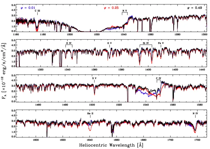
Figure 7 illustrates the three STIS spectra of CPD −28◦2561 that
Figure 7. STIS spectra of CPD −28◦2561 at three phases (0.01 in blue, 0.25 in red, and 0.49 in black), with identification of the key transitions.
see Fig. 1 for the orientation of the observer with respect to the magnetospheric structure inferred by Wade et al. (2015).
As discussed by Wade et al. (2015), the spectral type of CPD −28◦2561 varies between ∼O6.5 at its “high state” (which
corresponds to φ = 0.0 and 0.5, when Hα exhibits emission max-ima) and O8 at its “low state” (i.e. φ = 0.25 and 0.75). These classifications are based on the changes in the ratio of He i λ4471 to He ii λ4542, with the understanding that the low state proba-bly gives a better indication of the general properties of the stellar photosphere because the He i lines are partially filled with emis-sion during the high state. The line strengths in the UV spectra are broadly consistent with a “late O” classification, but are similarly characterized by significant abnormalities. In particular, the pres-ence of O v λ 1371 is atypical for the temperature classes indicated by the optical spectra, since it usually appears at similar strengths only at the earliest types (i.e., O2–O5). Its occurrence, together with the excessive strength of the N iv λ 1718 P Cygni profile indicates the presence of additional highly ionized gas. Another abnormal-ity concerns the Si iv doublet. As usual in spectra of mid-to-late O dwarfs, its components at phases 0.01 and 0.49 are absorption fea-tures with a strong interstellar contribution. However, the doublet becomes dramatically broader at φ = 0.25 (Hα minimum), which is anomalous when compared to the morphological trends exhibited by non-magnetic O-type stars.
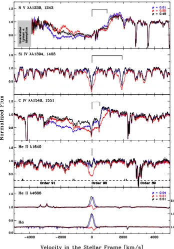
Finally, the most striking peculiarities occur in the P Cygni profiles of the N v and C iv doublets, which are significantly
dif-ferent at all three phases. These profiles are highlighted in Fig. 8, together with the Si iv doublet and He ii λ 1640 as well as spectra of He ii λ4686 and Hα obtained at similar phases by Wade et al. (2015). At all phases, the morphology of the P Cygni wind profiles is quite different from that expected for a spherically symmetric wind, primarily because of the weakness of the emission lobe.
The biggest changes in the UV spectra are seen at φ = 0.25, corresponding to Hα minimum - a time at which the line of sight to a distant observer passes through the material that collects near the magnetic equator. Enhanced absorption is visible in many lines at this phase, notably the Si iv doublet as already mentioned but also “photospheric” features like Fe v λ 1409 as well as diagnos-tics of circumstellar material like the C iii λ 1176 multiplet and the N iv λ 1718 line. The He ii λ 1640 line exhibits enormously en-hanced absorption at this phase, which is all the more noticeable because the line is either completely filled in by emission or dis-plays a weak P Cygni profile at both Hα maxima. The increased density along the line-of-sight at φ = 0.25 is evidently accompa-nied by changes in the velocity structure that reduce the amount of forward-scattered emission along the line of sight: this explains the enhanced absorption at low velocities in the P Cygni absorption trough of the N v and C iv doublets, which weakens the emission lobe and shifts the observed emission peak to longer wavelengths. The simultaneous enhancement of lines that arise from many differ-ent species and stages of ionization confirms that increased density
Figure 8. Normalized UV lines serving as diagnostics of the wind and
magnetosphere for three phases (0.01 in blue, 0.25 in red, and 0.49 in black). For comparison, the variations of He ii λ4686 and Hα at similar phases are shown at the same scale. The optical data were obtained with CFHT/ESPaDOnS (Wade et al. 2015).
is the primary cause of the increased optical depths, rather than changes in the ionization fractions.
Although the P Cygni profiles of the N v and C iv doublets show the presence of high-velocity material at all phases, the ab-sorption at high velocities is greatest near φ=0.01 when the fast polar wind is exposed (see Fig. 1 and Fig. 8). However, when the wind emerging from the opposite hemisphere is visible at phases near φ=0.49, the absorption trough is substantially reduced at all velocities even though the emission lobe is essentially identical in appearance. These differences, together with the similar strength but reversal in skew exhibited by Hα and He ii λ4686 at the two maxima (see Fig. 8 and Wade et al. 2015), indicate a significant asymmetry in the magnetosphere when viewed from these different perspectives.
4.2.1 Comparison with other magnetic massive stars
Although the oblique magnetic rotator model provides a useful conceptual basis for understanding the variability of stars like CPD −28◦2561, it is rich in parameters that determine how different
diagnostics appear and behave. For example, the detailed behavior of a resonance line in a magnetic O-type star depends on the mass flux from the surface of the underlying star, the stellar rotation rate,
the strength and geometry of the magnetic field, the competition be-tween radiative, magnetic, and centripetal forces on the ionization balance in both the magnetosphere and the free-streaming wind, and the observer viewing aspect α (see last column of Table 1). De-spite the diversity of this parameter space and the current difficulty to get UV spectra, some patterns of behaviour for ultraviolet diag-nostics are starting to emerge as more phase-resolved spectroscopy becomes available.
UV spectroscopy is currently available for three Of?p stars (HD 108, HD 191612, and CPD −28◦2561, Marcolino et al.
2012, 2013, and this work), HD 57682 (Grunhut et al. 2009), and the young magnetic O-star θ1Ori C (Stahl et al. 1996;
Smith & Fullerton 2005).
The Of?p stars HD 191612 and HD 108 display weaker P Cygni profiles (i.e. less blueshifted absorption and more red-shifted absorption) of strong UV lines when the Hα emission is minimum (hence equatorial regions are seen edge-on) while weaker UV lines, having no blueshifted absorption, show only stronger low-velocity absorptions at this phase (Marcolino et al. 2012, 2013). For HD 108, the strong lines were N v λ 1240, Si iv λ 1400, C iv λ 1550, and N iv λ 1718, while the Fe iv forest fell in the weak line category. For HD 191612 as for CPD −28◦2561, Si iv λ 1400
changed category, hence changed behaviour. This dichotomy could be qualitatively reproduced by MHD simulations (see Fig. 6 of Marcolino et al. 2013). Strong lines, such as those of C iv, are sen-sitive even to the high-speed wind flowing out of the poles, despite its lower density compared to the confined plasma of the equato-rial regions. Therefore, such lines display absorption over a large range of velocities. They can be broadly described as P Cygni pro-files, which become stronger when the system is seen pole-on (and the free-flowing polar wind comes into view). When the equatorial region is seen edge-on, the line-of-sight absorbing column mostly traces the dynamical magnetosphere region characterized by low velocities, so that the P Cygni profiles appear globally weaker. In contrast, intrinsically weak lines are not sensitive to the outflow-ing wind, so they exhibit less or even negligible absorption at high velocities and display a simple absorption profile located at low velocities. This absorption logically increases when the dense and slowly-moving confined winds of the equatorial regions enter the line-of-sight. In this framework, CPD −28◦2561 appears as both
similar and different. Indeed, purely photospheric lines are con-stant while low-velocity absorptions are indeed stronger at φ=0.25, when the dense equatorial regions enter the line-of-sight. However, the changes in C iv (in particular its different profiles at the two maxima) and He ii are novel.
Outside the Of?p category, the reported behaviours are quite varied. The magnetic O-type star HD 57682 seems perfectly in line with Of?p stars, as its Si iv doublet displays stronger and broader absorptions at Hα minimum (see Fig. 4 of Grunhut et al. 2009, considering ephemeris of Grunhut et al. 2012). However, the situa-tion appears somewhat different for θ1Ori C. While the absorption
in Si iv λ 1400 increases when the magnetic equator is seen edge-on, the C iv and N v lines display an opposite behaviour compared to Of?p stars (Smith & Fullerton 2005): these lines have enhanced blueshifted absorption when Hα emission is minimum (hence equa-tor is seen edge-on) and enhanced absorption at lower velocities when Hα emission is maximum (face-on view of the equatorial re-gions). The reason for this opposite behaviour is not yet known.
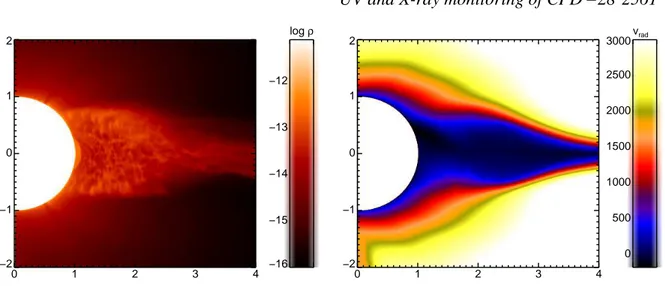
0.00.20.40.60.81.0 −16 −15 −14 −13 −12 −16 −15 −14 −13 −12 0 1 2 3 4 −2 −1 0 1 2 0 1 2 3 4 −2 −1 0 1 2 log ρ 0.00.20.40.60.81.0 0 500 1000 1500 2000 2500 3000 0 500 1000 1500 2000 2500 3000 0 1 2 3 4 −2 −1 0 1 2 0 1 2 3 4 −2 −1 0 1 2 vrad
Figure 9. Plots of logarithmic density (left) in g cm−3and radial velocity (right) in km s−1, computed by averaging 122 zones in azimuth for a snapshot of the 3-D radiation MHD wind simulation described in the text. The x- and y-axes are both scaled to units of R∗, and the magnetic north pole is located to the top at x = 0.
4.2.2 Modelling of the UV spectrum
We now interpret the UV observations described in the previous subsections by considering the structure of the magnetically con-fined winds in CPD −28◦2561, for which η
∗amounts to ∼230 and
RA to ∼ 4.2 R∗(Table 4). We use a snapshot of a full 3-D
numer-ical radiation magnetohydrodynamic (MHD) simulation that fol-lows the dynamics of an O-star wind possessing a large-scale dipo-lar magnetic field, hence a dipo-large η∗of ≈ 100, as described in
de-tail by ud-Doula et al. (2013, see also Fig. 9). This model was ini-tially calculated for HD 191612 but since its properties are simi-lar to those of CPD −28◦2561, the model can directly be applied
to the latter star (taking into account the uncertainties, see Table 4). A key aspect of the model is the over-dense region around the magnetic equator, which is characterized by quite low veloc-ities when compared to the free-flowing wind of a non-magnetic O star. Considering the geometry of the specific system under in-vestigation, this general model of a dynamical magnetosphere has been able to reproduce the rotational modulation of the Hα line of CPD −28◦2561 (Wade et al. 2015), but also of other magnetic
O-stars (Sundqvist et al. 2012; Grunhut et al. 2012; ud-Doula et al. 2013; Petit et al. 2013). Note however that, in addition to the mag-netically confined plasma in the closed equatorial loops, the strong UV wind lines studied here depend also on the wind outflow in the open field regions (see Fig. 1 and Marcolino et al. 2013).
To compute synthetic UV resonance line-profiles from our MHD simulation, we describe the opacity by the parameter (e.g., Puls, Owocki & Fullerton 1993):
k0= q ˙MB=0 R∗v2∞ πe2/m ec 4πmH Ai 1 + 4YHe fluλ0. (1)
In this equation, YHe is the helium number abundance, fluthe
os-cillator strength of the transition, λ0its rest wavelength, q the ion
fraction of the considered element, Ai = ni/nHits abundance with
respect to hydrogen, and the other symbols have their conventional meaning.
An NLTE two-level atom scattering source function is then computed using the 3-D, local Sobolev method described, e.g., by Cranmer & Owocki (1996). Finally, we solve the formal solution of radiative transfer in a 3-D cylindrical system for an observer
−1000 0 1000 2000 3000 0.0 0.2 0.4 0.6 0.8 1.0 1.2 Normalized Flux −1000 0 1000 2000 3000 0.0 0.2 0.4 0.6 0.8 1.0 1.2 Normalized Flux −1.0 −0.5 0.0 0.5 1.0 0.0 0.5 1.0 1.5 Normalized Flux
Velocity in the Stellar Frame [km/s]
v/v∞ φ = 0.00 φ = 0.25 φ = 0.50 SiIV doublet Generic singlet
Figure 10. Synthetic UV line-spectra for the three observed phases. The
upper panel displays computations for the Si iv doublet, using k0 = 0.1,
while the lower panel shows a generic singlet profile with k0= 1, illustrative
of the C iv and N v lines. See text for discussion and model description.
viewing the magnetic axis with an angle α (see Table 1 and Fig. 1), following Sundqvist et al. (2012).
The top panel of Fig. 10 displays the synthetic UV line profiles for the (clearly separated) lines of the Si iv doublet. We have here used photospheric profiles from a tlusty model atmosphere (Lanz & Hubeny 2003), for the stellar parameters in Table 4 and convolution by an isotropic 40 km s−1macroturbulence
(Sundqvist et al. 2013), as a lower boundary condition to our radiative transfer computations. However, our code cannot treat overlapping resonance doublets, such as C iv and N v: neglecting the underlying photospheric profiles, these lines are instead discussed in terms of a generic singlet line of approximately the same observed line strength.
Line strengths and ion balance. The observed wind lines are
sur-prisingly weak for an O star corresponding to the parameters given in Table 4. The Si iv lines require an opacity parameter k0 . 0.1
too strong. In addition, and perhaps more importantly, both the C iv and N v P Cygni lines are unsaturated. While the faster-than-radial divergence of the magnetic polar wind (Owocki & ud-Doula 2004) results in line profiles that are weaker than in corresponding non-magnetic winds (see Marcolino et al. 2013, their Fig. 6), test com-putations show that both the absorption trough and emission peak of the C iv and N v lines become too strong when k0 is increased
by factors of a few above unity. Inserting in eqn. 1 appropriate line strengths (as used in Fig. 10) and other relevant parameters, and adopting a solar Si abundance and N and C abundances as es-timated by Wade et al. (2015), give for the product of ionization fraction and mass feeding rate, hq ˙MB=0i ≈0.4, 6, 9 × 10⁻⁹M⊙/yr
for Si iv, C iv, N v, respectively. Assuming then ˙MB=0according to
the scaling formula by Vink, de Koter & Lamers (2000, see Table 4), this gives order-of-magnitude estimates for ion fractions hqi of about ∼0.01 for C iv and N v, and . 0.001 for Si iv.
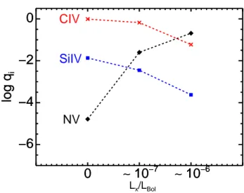
Unfortunately, as of today there exists no proper NLTE code for calculating the ion balance in a non-spherical, magnetic O-star wind, where most likely the distribution of X-rays also is highly as-pherical (see previous sections). As a first approximation, however, we have computed ionization models by means of the spherically symmetric NLTE fastwind code (Puls et al. 2005), using a newly implemented treatment of X-rays (Carneiro et al., in prep., essen-tially following Pauldrach et al. 1994 and Feldmeier et al. 1997). Fig. 11 displays the computed ion fractions at a characteristic ra-dius r = 2R∗, for three different models with Lx/LBolratios in the
0.4-2.5 keV energy band of 0, ∼ 10−7, and ∼ 10−6.
Focusing on the well developed – but unsaturated – C iv and N v wind lines, the figure shows that without any X-ray ioniza-tion the C iv (resp. N v) ion fracioniza-tions are far too high (resp. low) compared to observationally-derived values. Introducing Lx/LBol∼
10−7does not significantly improve the situation, since C iv remains
the main ion stage. As the X-ray luminosity increases, C iv starts to be ionized away, whereas the fraction of N v steadily increases. Since the C iv and N v lines are unsaturated and of similar strength, this anti-correlated behaviour of their ion fractions is a potentially important clue for understanding the strength of the UV wind lines in CPD −28◦2561 and similar magnetic stars.
Since the C iv and N v lines are observed to be of approxi-mately equal strengths, their ion fractions must also be roughly equal. From Fig. 11, we see this occurs in our models for a
Lx/LBol ∼ 10−6.3, significantly higher than the canonical value of
10−7for non-magnetic O-stars (Berghoefer et al. 1997; Naz´e 2009;
Naz´e et al. 2011), in general agreement but still slightly below the observed X-ray luminosity for CPD −28◦2561 (log[L
X/LBOL]
∼ −6.1 in that bandpass, see models of Section 3). The Si iv ion fraction is then q ∼ 0.001, as derived above, but the C iv and N v ion fractions are q ∼ 0.1, while we instead derived values of
∼0.01, assuming a mass-loss feeding rate from Vink’s formula. Matching the C iv and N v line profiles with q ∼ 0.1 would require the ˙MB=0assumed above be reduced by approximately an order of
magnitude. This result is similar to that found by Marcolino et al. (2013) for HD 191612, but it should be kept in mind that the ion fractions presented here are valid only at a certain characteristic radius whereas the real q in the non-spherical, magnetic wind will certainly vary both with radius and latitude. As such, these tentative results need to be tested by more direct comparisons to the observed line profiles, using a new, future set of improved models.
Variability. As discussed by Marcolino et al. (2013), the
line-of-sight absorption column when viewed from above the magnetic
0
∼
10
−7∼
10
−6−6
−4
−2
0
log q
i0
∼
10
−7∼
10
−6−6
−4
−2
0
log q
i Lx/LBolCIV
SiIV
NV
Figure 11. Theoretical calculations of the logarithms of ion fractions qi for i = C iv, Si iv, and N v (labelled in the figure) at a characteristic radius r = 2R∗in fastwind models using three different Lx/LBolratios (see text for details).
equator samples the high density wind material of the magneto-sphere, which is characterized by rather low velocities and some infall. By contrast, the absorption column from an observer above the magnetic pole samples the free-streaming and fast polar wind. This leads to stronger absorption at high (resp. low) velocities when viewed closer to the magnetic pole (resp. equator). Even though we never view CPD −28◦2561 from directly above the magnetic pole
(Table 1 and Fig. 1), this quite general behavior is preserved. It ex-plains the stronger absorptions seen at low velocities for φ=0.25 in the He ii, Si iv, and C iv lines (Figs. 7 and 8), while the absorption difference at high velocities between the φ=0.25 (equator-on) and
φ=0.5 views is reduced in the generic line profile (bottom panel of Fig. 10 to be compared with third panel of Fig. 8). However, the observed weak silicon lines are also highly influenced by the inter-stellar absorption and photospheric profile. In our models, the lat-ter lowers the scatlat-tering emission component and brings these lines into pure absorption. Overall, our synthetic line profiles and their variability are in good qualitative agreement with the observed pro-files in Fig. 8, providing further strong support for the general “dy-namical magnetosphere” paradigm for magnetized O-star winds.
There are some potentially important deviations between models and observations, however. For example, the change in width of the Si iv line is quantitatively larger in the STIS obser-vations. In addition, the large difference in absorption at high ve-locities in the C iv and N v lines during phases 0.0 and 0.5 indi-cates strong asymmetries about the magnetic equator. While tran-sient asymmetries are seen in our 3D MHD simulations (see also ud-Doula et al. 2013), their corresponding effect on the synthetic line profiles in Fig. 10 is barely visible and as such is much weaker than observed. It is interesting to note that these observed absorp-tion differences between equal viewing angles toward the southern and northern hemispheres occur mainly at high blueshifted veloc-ities, suggesting (somewhat surprisingly) that the free streaming wind might be more affected by such symmetry-breaking than the confined dynamical magnetosphere.
5 CONCLUSION
We have examined the high-energy emission of the Of?p star CPD −28◦2561, and its variations, using XMM-Newton and HST
observations. In this system, the magnetic field is able to confine the stellar wind flows near the magnetic equator, forming a dynam-ical magnetosphere surrounding the star. With angles of inclina-tion and obliquity of (90◦, 35◦) or (35◦, 90◦), the magnetosphere
of CPD −28◦2561 is seen edge-on twice per rotation period
(corre-sponding to minimum emissions in the optical) and nearly face-on twice per period (corresponding to maximum emissions in the op-tical). The XMM-Newton observations sample both maxima and minima, as well as an intermediate phase; the HST observations sample both maxima and the first minimum.
In X-rays, CPD −28◦2561 displays a bright (log[L
X/LBOL]∼
−5.8) and hard (hard-to-soft flux ratio close to one) emission. The X-ray emission is both brighter and harder than in other Of?p stars. This emission remains stable on short timescales, but the X-ray flux varies by ∼55% with rotational phase, a value similar to what is seen in the Of?p star HD 191612 or in the O-star θ1Ori C. These
phase-locked changes closely follow the variations of the optical emission lines, i.e. there are two maxima and two minima in X-rays during the 73d rotational period of CPD −28◦2561, as expected for
a magnetic oblique rotator. There is no significant hardness varia-tion except for the last observavaria-tion, taken during the second mini-mum. In view of the stability of the behaviour in the optical domain, this change is probably linked to an asymmetry in the magneto-sphere.
In the UV domain, two types of data are available: photom-etry taken by the OM telescope aboard XMM-Newton and high-quality HST-STIS spectroscopy. These observations reveal that CPD −28◦2561 displays a stable broad-band flux as well as
sta-ble “photospheric” lines. However, large profile variations of the lines associated with the circumstellar environment are detected in the UV spectra. First, enhanced absorption at low velocities is ob-served when the magnetic equatorial regions are seen edge-on. This increase in absorption, particularly spectacular for the He ii λ 1640 line, is directly due to the presence of dense plasma projected onto the stellar disk. It is reproduced qualitatively by detailed 3D mod-elling of a magnetically confined wind. Second, a difference also exists in the high-velocity absorption of the C iv and N v P Cygni profiles when comparing the two phases corresponding to the two maxima of the optical emissions. This strong variation in profile appears surprising as the optical emissions at the same phases have similar strengths, but it nevertheless suggests the presence of asym-metries in the north vs the south magnetic hemispheres. As the dif-ference appears at high velocities while the confined winds have low velocities, these asymmetries should be more prevalent in the free-flowing wind. However, the origin of these asymmetries and their link with the magnetic field remains to be established. Finally, we note that empirically derived ion fractions require a significantly higher Lx/LBolratio than the canonical value 10−7for non-magnetic
O-stars, in agreement with the detailed X-ray analysis, but that re-producing the overall strengths of the UV wind lines with these ion fractions then requires a ˙MB=0that is significantly lower than
expected.
ACKNOWLEDGMENTS
YN & GR acknowledge support from the Fonds National de la Recherche Scientifique (Belgium), the PRODEX XMM con-tract, and an ARC grant for Concerted Research Action financed
by the Federation Wallonia-Brussels. JOS acknowledges support from SAO Chandra grant TM3-14001A. AuD acknowledges sup-port by NASA through Chandra Award number TM4-15001A and 16200111 issued by the Chandra X-ray Observatory Center which is operated by the Smithsonian Astrophysical Observatory for and behalf of NASA under contract NAS8- 03060. AuD, AWF, and NRW acknowledge support for Program number HST-GO-13629 that was provided by NASA through a grant from the Space Tele-scope Science Institute. GAW acknowledges Discovery Grant sup-port from the Natural Science and Engineering Research Council (NSERC) of Canada. The authors also acknowledge help and dis-cussion with Rodolfo Barb`a and V´eronique Petit. We thank Luiz Carneiro for making a new version of FASTWIND available to us prior to final publication. ADS and CDS were used for preparing this document.
REFERENCES
Asplund, M., Grevesse, N., Sauval, A. J., & Scott, P. 2009, ARA&A, 47, 481
Babel, J., & Montmerle, T. 1997a, A&A, 323, 121
Barannikov, A. A. 2007, Information Bulletin on Variable Stars, 5756, 1
Barb´a, R. H., Gamen, R., Arias, J. I., et al. 2010, Revista Mexicana de Astronomia y Astrofisica Conference Series, 38, 30
Barb´a, R., Gamen, R., Arias, J. I., et al. 2014, Revista Mexicana de Astronomia y Astrofisica Conference Series, 44, 148 Berghoefer, T. W., Schmitt, J. H. M. M., Danner, R., & Cassinelli,
J. P. 1997, A&A, 322, 167
Bohlin, R. C., Savage, B. D., & Drake, J. F. 1978, ApJ, 224, 132 Cranmer, S. R., & Owocki, S. P. 1996, ApJ, 462, 469
Donati, J.-F., Howarth, I. D., Jardine, M. M., et al. 2006, MNRAS, 370, 629
Feldmeier A., Kudritzki R.-P., Palsa R., Pauldrach A. W. A., Puls J., 1997, A&A, 320, 899
Gagn´e, M., Oksala, M. E., Cohen, D. H., et al. 2005, ApJ, 628, 986 (see erratum in ApJ, 634, 712)
Garrison, R. F., Hiltner, W. A., & Schild, R. E. 1977, ApJS, 35, 111
Grunhut, J. H., Wade, G. A., Marcolino, W. L. F., et al. 2009, MNRAS, 400, L94
Grunhut, J. H., Wade, G. A., Sundqvist, J. O., et al. 2012, MN-RAS, 426, 2208
Hubrig, S., Sch¨oller, M., Kharchenko, N. V., et al. 2011, A&A, 528, AA151
Hubrig, S., Kholtygin, A., Scholler, M., et al. 2012, Information Bulletin on Variable Stars, 6019, 1
Hubrig, S., Sch¨oller, M., Kholtygin, A. F., et al. 2015, MNRAS, 447, 1885
Jansen, F., Lumb, D., Altieri, B., et al. 2001, A&A, 365, L1 Lanz T., Hubeny I., 2003, ApJS, 146, 417
Marcolino, W. L. F., Bouret, J.-C., Walborn, N. R., et al. 2012, MNRAS, 422, 2314
Marcolino, W. L. F., Bouret, J.-C., Sundqvist, J. O., et al. 2013, MNRAS, 431, 2253
Martins, F., Donati, J.-F., Marcolino, W. L. F., et al. 2010, MN-RAS, 407, 1423
Mason, K. O., Breeveld, A., Much, R., et al. 2001, A&A, 365, L36
Naz´e, Y. 2009, A&A, 506, 1055
Naz´e, Y., Rauw, G., Vreux, J.-M., & De Becker, M. 2004, A&A, 417, 667
Naz´e, Y., Barbieri, C., Segafredo, A., Rauw, G., & De Becker, M. 2006, IBVS, 5693
Naz´e, Y., Rauw, G., Pollock, A. M. T., Walborn, N. R., & Howarth, I. D. 2007, MNRAS, 375, 145
Naz´e, Y., Walborn, N.R., Rauw, G., Martins, F., Pollock, A.M.T., & Bond, H.E. 2008a, AJ, 135, 1946
Naz´e, Y., Walborn, N. R., & Martins, F. 2008b, Revista Mexicana de Astronomia y Astrofisica, 44, 331
Naz´e, Y., ud-Doula, A., Spano, M., et al. 2010, A&A, 520, A59 Naz´e, Y., Broos, P. S., Oskinova, L., et al. 2011, ApJS, 194, 7 Naz´e, Y., Oskinova, L. M., & Gosset, E. 2013, ApJ, 763, 143 Naz´e, Y., Petit, V., Rinbrand, M., et al. 2014a, ApJS, 215, 10 Naz´e, Y., Wade, G. A., & Petit, V. 2014b, A&A, 569, A70 Owocki S. P., ud-Doula A., 2004, ApJ, 600, 1004
Pauldrach A. W. A., Kudritzki R. P., Puls J., Butler K., Hunsinger J., 1994, A&A, 283, 525
Petit, V., Owocki, S. P., Wade, G. A., et al. 2013, MNRAS, 429, 398
Puls J., Owocki S. P., Fullerton A. W., 1993, A&A, 279, 457 Puls J., Urbaneja M. A., Venero R., Repolust T., Springmann U.,
Jokuthy A., Mokiem M. R., 2005, A&A, 435, 669 Smith, M. A., & Fullerton, A. W. 2005, PASP, 117, 13 Stahl, O., Kaufer, A., Rivinius, T., et al. 1996, A&A, 312, 539 Stelzer, B., Flaccomio, E., Montmerle, T., et al. 2005, ApJS, 160,
557
Str¨uder, L., Briel, U., Dennerl, K., et al. 2001, A&A, 365, L18 Sundqvist J. O., Petit V., Owocki S. P., Wade G. A., Puls J.,
MiMeS Collaboration, 2013, MNRAS, 433, 2497
Sundqvist J. O., ud-Doula A., Owocki S. P., Townsend R. H. D., Howarth I. D., Wade G. A., 2012, MNRAS, 423, L21
ud-Doula A., Owocki S. P., 2002, ApJ, 576, 413
ud-Doula A., Owocki S. P., Townsend R. H. D., 2008, MNRAS, 385, 97
ud-Doula, A., Owocki, S. P., & Townsend, R. H. D. 2009, MN-RAS, 392, 1022
ud-Doula A., Sundqvist J. O., Owocki S. P., Petit V., Townsend R. H. D., 2013, MNRAS, 428, 2723
ud-Doula, A., Owocki, S., Townsend, R., Petit, V., & Cohen, D. 2014, MNRAS, 441, 3600
Turner, M. J. L., Abbey, A., Arnaud, M., et al. 2001, A&A, 365, L27
Vink J. S., de Koter A., Lamers H. J. G. L. M., 2000, A&A, 362, 295
Wade, G. A., Barb´a, R. H., Grunhut, J., et al. 2015, MNRAS, 447, 2551
Walborn, N.R. 1972, AJ, 77, 312 Walborn N.R. 1973, AJ, 78, 1067
Walborn, N. R., Lennon, D. J., Heap, S. R., et al. 2000, PASP, 112, 1243
Walborn, N.R., Howarth, I.D., Rauw, G., et al. 2004, ApJ, 617, L61
Walborn, N. R., Sota, A., Ma´ız Apell´aniz, J., et al. 2010, ApJ, 711, L143
This paper has been typeset from a TEX/ LATEX file prepared by the