Combining microsatellite and pedigree data to estimate relationships among Skyros ponies.

Introduction

Numerous methods for computing inbreeding and relationship coefficients are available. The first type of methods is based on genealogical informa-tion. These methods can be classified into 2 cate-gories (Boichard et al. 1996): (1) methods that consider the founders as unrelated and non-inbred (e.g. Wright 1922; Henderson 1976 or Meuwissen and Luo 1992), and (2) methods that consider the founders as potentially related and inbred (e.g. VanRaden 1992). These relationship coeffi-cients are traditionally calculated on the basis of the pedigree of the breed. However, in many situa-tions, complete pedigrees are not available for a

significant fraction of the individuals in the stud-ied population or even for the whole population. Consequently, in recent years, scientists have be-come interested in the use of genetic markers to determine the genealogical relationships present in populations (Pamilo and Crozier 1982). Thus, the second type of methods is based on molecular markers, such as microsatellites. They also can be classified into 2 groups: (1) methods that use mo-ment estimators to estimate the relatedness be-tween pairs of individuals (e.g., Queller and Goodnight 1989; Li et al. 1993; Lynch and Ritland 1999), and (2) methods that use a likelihood ap-proach to allocate pairs or groups of individuals to relationship categories, such as full-sibs, par-J Appl Genet 50(2), 2009, pp. 133–143

Original article

Combining microsatellite and pedigree data to estimate

relationships among Skyros ponies

E. Bömcke1,2, N. Gengler1,3 1

Animal Science Unit, Gembloux Agricultural University, Passage des Déportés, Gembloux, Belgium 2

F.R.I.A., Rue d’Egmont, Brussels, Belgium 3

National Fund for Scientific Research, Rue d’Egmont, Brussels, Belgium

Abstract. Relationship coefficients are particularly useful to improve genetic management of endangered popu -lations. These coefficients are traditionally based on pedigree data, but in case of incomplete or inexistent pedi-grees they are replaced by coefficients calculated from molecular data. The main objective of this study was to develop a new method to estimate relationship coefficients by combining molecular with pedigree data, which is useful for specific situations where neither pedigree nor molecular data are complete. The developed method was applied to contribute to the conservation of the Skyros pony breed, which consists of less than 200 individuals, di-vided into 3 main herds or subpopulations. In this study, relationships between individuals were estimated using traditional estimators as well as the newly developed method. For this purpose, 99 Skyros ponies were genotyped at 16 microsatellite loci. It appeared that the limitation of the most common molecular-based estimators is the use of weights that assume relationships equal to 0. The results showed that, as a consequence of this limitation, nega-tive relationship values can be obtained in small inbred populations, for example. By contrast, the combined esti-mator gave no negative values. Using principal component analysis, the combined estiesti-mator also enabled a better graphic differentiation between the 3 subpopulations defined previously. In conclusion, this new estimator can be a promising alternative to traditionally used estimators, especially in inbred populations, with both incomplete pedigree and molecular information.

Keywords: microsatellites, pedigree, relationships, Skyros pony.

Received: August 6, 2008. Revised: December 11, 2008. Accepted: December 17, 2008.

Correspondence: E. Bömcke, Gembloux Agricultural University, Animal Science Unit, Passage des Déportés 2, B-5030 Gembloux, Belgium; e-mail: bomcke.e@fsagx.ac.be

ent-offspring, etc. (e.g., Mousseau et al. 1998; Goodnight and Queller 1999; Thomas and Hill 2002).

Knowledge of relationships among animals is useful for both the study of wild populations and the genetic management of captive and/or threat-ened populations (Glaubitz et al. 2003). In wild populations, relationships can be used in studies of kin selection, social behavior and social organiza-tion (e.g. Morin et al. 1994). Furthermore, this knowledge is also useful in research concerning mating systems (e.g. Heg and van Treuren 1998; Engh et al. 2002), dispersal, isolation by distance, and special genetic structure (e.g. Goodisman and Crozier 2002), and for the estimation of quantita-tive genetic parameters, such as heritability (Mousseau et al. 1998; Ritland 2000). In captive populations, knowledge of relationships and shared ancestry enables the minimization of in-breeding by permitting matings only between the most distantly related individuals (e.g. Jones et al. 2002). The knowledge of the relationship coeffi-cients is thus one of the principal tools used to op-timize conservation strategies (Hedrick and Miller 1992; Rochambeau et al. 2000; Caballero and Toro 2002; Verrier et al. 2005).

In reality, both sources of information are often incomplete or limited. An example of this situa-tion is the Skyros pony, a Greek indigenous horse breed, mainly found on the island of Skyros. The risk status of this breed is described as criti-cal-maintained, according to the criteria estab-lished by the Food and Agriculture Organization (FAO 1998; DAD-IS 2007). The small size of this population, about 200 individuals concentrated in 3 main subpopulations (Skyros, Corfu and Thessaloniki), and the linked risk of demographic accidents, are major factors that explain this sta-tus. The studbook of the breed includes animals recorded for 10 to 20 years. The pedigree depth is thus not sufficient to estimate accurately the rela-tionships, as many individuals have unknown par-ents. An accurate estimation of relationships among individuals from molecular data is also dif-ficult. Indeed, the number of genotyped individu-als and of markers is limited essentially for budgetary reasons. So combining molecular and pedigree data could permit a better estimation of the relationships among individuals than estima-tion based on only one type of available data.

Although molecular markers are available for most species for several years, it is interesting to note that so far no studies have tried to combine both sources of information into one single esti-mator. In our study, the idea was therefore to

de-velop a combined estimator. The choice to com-bine the 2 types of coefficient was made for 2 rea-sons. Firstly, if only the results of the DNA analysis are used to estimate the relatedness, indi-viduals are related only for known markers. DNA analyses allow “telling the historical review of the breed”. If only the pedigree data are used, it does not enable retracing all the history of the breed, but it is very informative for the close parents. Conse-quently, the simple replacement of the pedi-gree-based coefficients by molecular-based coefficients leads to a loss of information. Sec-ondly, a limitation of the common molecu-lar-based estimators was the use of weights that assume zero relationship. Thus including the known pedigree relationship in the estimation, al-lowed to correct the molecular coefficients for the relations existing in the studied population.

With regard to conservation breeding pro-grams, it seems essential to use pedigree informa-tion whenever available, especially when the costs of genotyping for a high number of microsatellite markers are considered. But the situation might change if genotyping costs could be reduced in the near future. Meanwhile, DNA technologies are not suitable to replace a studbook (Baumung and Sölkner 2003).

In conclusion, the main objective of this study was to improve the calculation of relationship val-ues by developing a method combining pedigree and marker data, using the endangered Skyros pony breed as a reference population.

Materials and methods

Source of information

A preliminary studbook for Skyros pony was es-tablished very recently and includes 395 animals, born between 1958 and 2006. A previous study showed that the Skyros population consists of 3 subpopulations: Skyros (about 100 individuals), Thessaloniki (50 individuals) and Corfu (30 indi-viduals) (Bömcke 2007). The completeness of pedigree information was characterized by com-puting the number of generation-equivalents (geq). This parameter is often considered as the best criterion to characterize the quality of the ped-igree information (Maignel et al. 1996; Baumung and Sölkner 2003). The geq was computed for each animal as the sum of (1/2)n, where n is the number of generations separating the individual from each known ancestor (Huby et al. 2003).

DNA samples were collected from 99 ponies: 37 males and 62 females. The sampled animals

were born between 1982 and 2006 and represented the 3 herds: Skyros (50 individuals), Thessaloniki (25 individuals) and Corfu (24 individuals). The samples were tested for genetic variation at 16 loci on 12 different chromosomes with microsatellite markers, recommended for parentage testing by the International Society of Animal Genetics (ISAG) Equine Genetics Standing Committee. The microsatellites were the following: VHL20, HTG04, AHT04, HMS07, HTG06, AHT05, HMS06, ASB23, ASB02, HTG07, HMS03, HMS02, ASB17, LEX03, HMS01 and CA425 (Dimsoski 2003).

Definition of pedigree relationship coefficients

Basing on pedigree records, the construction of the additive relationship matrix was performed recur-sively, using the tabular method as described by Van Vleck et al. (1987). Additive relationships were sequentially established from oldest to youn-gest animals. Founders (i.e. animals without known parents) were considered as unrelated and non-inbred. Lets x and y denote a pair of individu-als, p and q denote the parents of y, and axydenote the additive relationship coefficient among x and y. It is assumed that axy= ayx= 0.5(axp+ axq) for x¹y (Henderson 1976). The inbreeding coefficient of y is calculated as a half of the additive relationship between its parents (p and q). It follows that Fy= 0.5apqand the additive relationship of y with itself is ayy=1+ Fy.

The additive relationships (axy) were trans-formed into Wright et al. (1925) relationship coef-ficients (rxy), according to the following equation: The obtained relationship, also called numerator relationship, is independent from the inbreeding coefficient of individuals x and y. This transforma-tion allows the relatransforma-tionship coefficient to be a measure of the degree to which the genotypes of x and y are similar, rather than leave it in terms of the proportion of genes from a common source (Minvielle 1990).

Definition of molecular relationship coefficients

Basing on microsatellites, the total allelic relation-ship (TA) of the 2 alleles of an individual with the 2 alleles of the other individual was calculated for each locus (l): TAxy,l= 2 × fMxy,l

The coefficient of 2 emphasizes that TA is twice the relationship coefficient (Malécot 1948) and is analogous to the numerator relationship (Wright 1922) calculated from the pedigree.

The fM is the molecular co-ancestry between 2 individuals (Caballero and Toro 2000; Eding and Meuwissen 2001). By definition, it is the probability that 2 alleles taken randomly (one from each individual) are identical-by-descent (IBD). This coefficient has the advantage of being defined in a similar way as the classical Malécot coefficient (Toro et al. 2002). The fM can be writ-ten as: fMxy,l= 1/4[Sac+ Sad+ Sbc+ Sbd]

where the subscript l indicates the locus, the sub-scripts a, b, c and d indicate allelic position 1 of l of individual x, allelic position 2 of l of x, allelic posi-tion 1 of l of individual y, and allelic posiposi-tion 2 of l of y, respectively, and S.. refers to values depend-ing on whether alleles at the allelic positions in the subscript are the same (S..=1) or not (S..=0).

The locus-specific relationship can be further averaged over L loci:

TA TA L xy l l L =

å

Thereafter, TAXYwas transformed into rmol,xyby the following equation:

r_{mol xy}, =TAxy / TAxx ´TAyy

where TAxxand TAyydenote the total allelic iden-tity of the individuals x and y with themselves. The obtained relationship matrix (Rmol) was thus com-parable to the pedigree-based relationship matrix (Rped).

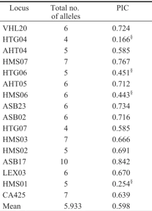
Two different Rmolmatrices were constructed: the first one based on all the 16 microsatellites of the marker set, and the second one based only on markers that were highly informative (PIC > 0.5), i.e. 12 microsatellites (Table 1).

Relationship estimation using DNA and pedigree 135

Table 1. Total number of alleles and polymorphism information content (PIC) of the 16 microsatellites

Locus Total no. of alleles PIC VHL20 6 0.724 HTG04 4 0.166§ AHT04 5 0.585 HMS07 7 0.767 HTG06 5 0.451§ AHT05 6 0.712 HMS06 6 0.443§ ASB23 6 0.734 ASB02 6 0.716 HTG07 4 0.585 HMS03 7 0.666 HMS02 5 0.691 ASB17 10 0.842 LEX03 6 0.670 HMS01 5 0.254§ CA425 7 0.639 Mean 5.933 0.598 §

Loci excluded from construction of matrix based on highly informative loci (PIC<0.5)

Definition of a new combined relationship coefficient

In an ideal situation, the whole pedigree is known and relationship calculations are based on statisti-cal assumptions about genes shared between indi-viduals. Thus, the more information is available from the pedigree, the less molecular information is needed. The other extreme situation is when very dense marker maps are available. According to VanRaden (2007), these molecular relation-ships, called then genomic relationrelation-ships, can re-place pedigree information completely. In practice, and especially in conservation genetics, intermediate situations are observed, where both pedigree and marker data are incomplete. Many pedigree records are not very reliable due to ran-dom mating between individuals with incomplete or no recording of the births. To use all available data, we combine the 2 relationship coefficients rped,xyand rmol,xyinto a single parameter rcomb, xy. As the relative quality of information needs to be inte-grated, rped,xyand rmol,xyshould be weighted using a function that is proportional to the quality of infor-mation. Theoretical weights can be developed bas-ing on the reciprocals of the error variances of relationship coefficient estimates. However, ob-taining these error variances is not evident; in fact, no method exists. Therefore, we used an empirical function of relative pedigree deepness as weight-ing factor for the pedigree relationship coeffi-cients. The following empirical weighting for the pedigree relationship coefficient between animals x and y was chosen and tested in this study:

(

)

(

)

(

(

)

)

w_xy = 1+geq_x ´ 1+geq_y / 2´ 1+ geq where geqi is the number of genera-tion-equivalents for the individual i (x or y), and geq represents the average number of genera-tion-equivalent for the analyzed population. For the animals that have the most complete pedigree, this function is close to 1, and for an animal with no pedigree record, this function is close to 0.

The molecular relationship coefficient was multiplied by the complementary value computed as 1-wx,yand by the average polymorphism infor-mation content (PIC) value. This last parameter was introduced by Botstein et al. (1980) and refers to the value of marker informativeness within a population, depending on the number of alleles and their frequencies.

Finally, the final formula of the new combined estimator is thus:

(

)

r_{comb xy,} =w_{x y,} ´r_{ped xy,} + 1-w_{x y,} ´PIC_mean´r_{mol xy,}

For comparison, a classic molecular relation-ship estimator was also computed, as proposed by Lynch and Ritland (1999). Their single-locus rela-tionship coefficient is:

( )

(

₍

)

₎₍

(

₎

)

where l indicates the locus, the subscripts a, b, c and d indicate allelic position 1 at locus l of indi-vidual x, allelic position 2 at locus l of x, allelic po-sition 1 at locus l of individual y, and allelic position 2 at locus l of y, respectively, paand pb de-note the population allele frequency of the alleles at allelic positions a and b, and S.. refers to values depending on whether alleles at the allelic posi-tions in the subscript are identical (S..=1) or not (S..=0). Multilocus estimates can be obtained as the sum of the single-locus estimates weighted by the inverse of their sampling variance, assuming zero relatedness, which equals:

( ) (

)(

)

The Lynch and Ritland estimator was chosen because it performed best in the studies of Van de Casteele et al. (2001) and Csilléry et al. (2006).

Example

Two genotyped individuals are chosen randomly: x and y.

The first individual (x) is a male coming from the Skyros herd. He was born in 1998. Its sire is unknown, its dam is known (Dx). For this animal, geq is equal to 0.5.

The second individual (y) is a female coming from the Corfu herd. She was born in 2004. Its sire is known (Sy), its dam is known (Dy). If we trace the complete pedigree of this animal, the corre-spondent geq is 1.938. For the genotyped popula-tion, the mean number of geq is 1.447.

Step 1: Calculation of the pedigree relationship coefficient:

Basing on the pedigree, there is no relation (1) between the parents of individual y (Sy and Dy) and individual x, then:

axy= ayx= 0.5*(axDy+ axSy) = 0.5*( 0 + 0) = 0 (2) between the parents of individual x (Sx and Dx, because Sx is unknown), and between the par-ents of individual y (Sy and Dy), then:

axx=1 = 1 + 0.5aSxDx= 1

ayy=1 + Fy= 1 + 0.5aSyDy= 1 + 0.5*0 = 1 It follows that:

r_{ped xy,} =a_xy / a_xx ´a_yy =0/ 1 1´ =0

Step 2: calculation of molecular relationship coefficient:

Based on the 2 microsatellite profiles (Table 2), TAxy,VHL20= 2*fMxy,VHL20= 1/2[Sac+ Sad+ Sbc+ Sbd] = 1/2[0 + 0 + 1 + 0] = 0.5

The same procedure is applied to all the microsatellites, TA is the average of the results for all microsatellites, therefore:

TAxy= 0.7 TAxx= 1.2 TAyy= 1.125 It follows that:

rmol, xy=TAxy/ TAxx ´TAyy=0.7/ 1 2 1125. ´ . =0.602

Step 3: Calculation of combined relationship coefficients

The weight is calculated from the following equation:

wx,y=

(

)

(

)

(

(

)

)

=

(

) (

)

(

(

)

)

rcomb,xy=wx,y× rped,xy+ (1–wx,y) × PICmean× rmol,xy = 0.430 × 0 + (1–0.430) × 0.598 × 0.602 = 0.205

Analysis of combined and traditional relationships

An analysis was conducted to quantify the dis-criminating power of the various relationship co-efficients, i.e. they were tested for their capacity to group the animals according to their herd of ori-gin. The underlying idea is that relationship coeffi-cients are one of the principal tools used to optimize conservation strategies; e.g. by permit-ting mapermit-tings only between the most distantly re-lated individuals and thus to minimize inbreeding. The geographic location of the 99 Skyros ponies was known and therefore could be used to test the discriminating power of the proposed measure of relationship. We conducted a principal component analysis (PCA) of 3 relationship matrices for the 99 animals. PCA makes it possible to reduce the number of dimensions, without much loss of infor-mation. In this study, PCA was used to present the results by scattered plots in 2-dimensional space, considering the first 2 principal components. We

applied for this purpose theFactorprocedure from SAS (1999).

Results and discussion

Pedigree deepness

Table 3 shows the number of genotyped individu-als per class of known geq. More than 25% of the individuals had less than one known geq, i.e. one or both parents were unknown. In these cases, cal-culating a relationship coefficient is impossible. Indeed, a common ancestor is necessary to calcu-late a relationship value between 2 individuals. When the pedigree is missing, the relationship co-efficient is considered to be zero. In this study, the mean number of geq is 1.447 and the maximum is 3.000, for an animal belonging to the Corfu subpopulation. These results showed well the ne-cessity to include the collected molecular data in calculation of relationships.

Limitation of the traditional estimator

The relatedness values calculated with Lynch and Ritland estimator ranged from –0.985 to 1.000, with a mean of –0.156. We observed that 76.71% of the values were negative. The conclusion was that Lynch and Ritland estimator underestimates the genealogical coefficients, as it was also shown by Toro et al. (2002) and Oliehoek et al. (2006).

Relationship estimation using DNA and pedigree 137

Table 2. Results of the genotyping kit for 2 chosen individuals (size of the alleles in nucleotides) o

VHL20 HTG4 AHT4 HMS7 HTG6 AHT5 HMS6 ASB23

x 86a 94b 130 132 157 157 172 178 85 95 133 135 165 167 188 190

y 94c 98d 130 130 157 159 170 172 95 95 137 133 161 167 188 190

ASB2 HTG7 HMS3 HMS2 ASB17 LEX3 HMS1 CA425

x 249 249 117 123 md* md 217 223 96 98 144 144 175 175 236 238

y 245 249 123 125 163 167 215 223 104 118 154 158 175 175 228 238

a,b,c and d_{used for the calculation of the molecular co-ancestry (fM) between x and y; *md = missing data}

Table 3. Percentage of genotyped individuals per class of known generation-equivalents (N=99)

Class of geq % of individuals

0.00–0.49 5.05 0.50–0.99 25.25 1.00 –1.49 16.16 1.50–1.99 28.28 2.00–2.49 15.15 ³2.50 10.10

The quality of Lynch and Ritland estimator data depends on several factors. These include the number of loci, the allelic frequency and, espe-cially, the degree of true relationship in the living population. One limitation of this estimator, and also of other common estimators of relatedness, is the use of weights that assume relationships in the population equal to zero. The best weight would be a function of the actual relationship (Lynch and Ritland 1999). A high level of relationship in the studied population could then explain the high percentage of negative values. Another limitation is that the allele frequencies are assumed to be the same as in the base population, which implies that there has been no change in gene frequencies. In Skyros ponies, it could not be assumed that the ac-tual frequencies of marker alleles were identical to those of the base population due to the genetic drift accumulated over years. In our opinion, the main explanation for the under-estimation, and the high percentage of negative values, seems to be the rel-atively high degree of actual relationship in the studied population and the lack of information on the true allelic frequencies in the base population.

Discriminating capacity of various estimators

Table 4 shows the percentage of information ex-plained by the first 3 principal components. The combined estimator showed the lowest total value, which is mainly due to the lower value for the first component, while the methods based on DNA alone led to higher values. TAxyshowed the highest

total value, and Lynch and Ritland estimator reached the highest value for the first principal component.

As mentioned previously, all individuals from the reference population can be considered as be-longing to 3 subpopulations. The repartition of genotyped individuals in these 3 subpopulations was known: a major group in Skyros (50 geno-typed individuals) and 2 smaller groups in Thessaloniki (25 genotyped individuals) and Corfu (24 genotyped individuals). This pattern should be reflected in the plot of the first 2 princi-pal components (axes).

Figure 1 shows the results of PCA of TAxy

coef-ficients. In spite of a high percentage of informa-tion explained by the first axis, the scattered plot showed no clear difference between the 3 groups of individuals.

Figure 2 shows the results of PCA of rR,xy

coef-ficients. Although this method showed the highest percentage of information explained by the first axis, the scattered plot showed a better distinction between the 3 groups of individuals.

Figure 3 shows the results of PCA of rcomb,xy,

based on 12 microsatellites. This method pre-sented a lower percentage of information ex-plained by the first axis than the 2 methods based on DNA alone. Nevertheless, the scattered plot showed a good distinction, with only few excep-tions, between the 3 groups of individuals. Except for one individual, the first axis differentiated the individuals of the Skyros subpopulation from the individuals of the other 2 subpopulations. The sec-ond axis differentiated, with few exceptions, the individuals of the Thessaloniki subpopulation from the individuals of the Corfu subpopulations. In the case of rcomb,xybased on 16 microsatellites,

the scattered plots (not shown) indicated the same as shown for 12 microsatellites, except that the distinction between the individuals from Thessaloniki and the individuals from Corfu was not evident. This was probably linked to the fact that highly polymorphic microsatellites allow to improve the distinction between individuals. In the case of combined estimator, where the Skyros subpopulation was separated from both other subpopulations, one individual belonging to the Corfu group was placed in the Skyros group of in-dividuals. The most plausible explanation is that this individual is the only one in the Corfu subpopulation, whose both parents were born in Skyros, and that this individual has no descendant. In the last case, the subpopulation of Thessaloniki was differentiated from the Corfu subpopulation with one exception. One individual belonging nor-mally to the Corfu group was found in the Thessaloniki group. The explanation for this ob-servation could be the same as described above, namely that both parents of this individual were born in Thessaloniki and that this individual has no descendant. In the other direction, 5 individuals belonging normally to the Thessaloniki group were considered as part of the Corfu group. A pos-sible explanation for this observation is that these animals were sent to Corfu Island. All their de-scendants were thus belonging to the Corfugroup and they were therefore regarded as being closer to this group than to their group of origin (Thessaloniki).

Table 4. Percentage of information explained by the first 3 principal components

Principal compo-nent TAxy Lynch & Ritland Combined (16 markers) Combined (12 markers) 1st 26.84% 29.06% 21.06% 21.37% 2nd 12.72% 10.18% 12.43% 11.62% 3rd 11.30% 9.22% 9.06% 8.82% Total 50.86% 48.46% 42.55% 41.81%

139

Figure 1. PCA representation of relationship coefficients obtained by calculation of TAxy(Sk=Skyros, Th=Thessaloniki,

Co=Corfu).

Additionally, in the case of combined estima-tor, it was interesting to note that the estimations based on the 12 highly informative microsatellite markers (PIC > 0.5) differentiated the sub-populations better that those based on 16, even if the percentages of information explained by the 3 axes were similar. These results showed that the use of the PIC value in the weighting has the po-tential to correct the value for the informative-ness of the markers. However, some improvements are necessary, e.g. the molecular relationship found for each locus should be multi-plied by the corresponding PIC value instead of using only the average value.

In spite of this weakness, the combined method for the estimation of relationship showed promising results, as compared to the other estimators. Another problem is the fact that the relationship coefficients are overesti-mated if DNA information is highly favoured in comparison to the pedigree information, but this is less the case than with other estimators. The fact that the combined estimator gave the most differentiated groups is a quality indicator, but this statement needs to be confirmed in forth-coming studies.

Use of the coefficients

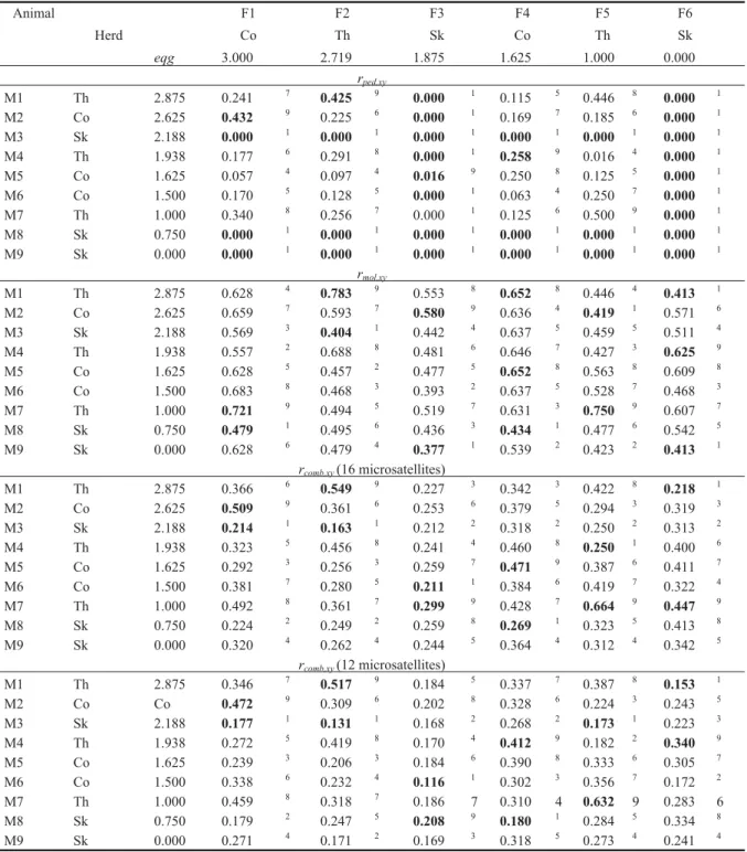
One aim of the study on Skyros pony was to help breeders to determine matings that minimize the in-crease in inbreeding within the population. For illus-tration, 6 females and 9 males were chosen: 2 females from each herd: one with the best-known pedigree and the other with the least-known pedigree of the herd, and 3 males of each herd: one with the best-known pedigree of the herd, one with the least-known, and one in between. Table 5 shows the relationship coefficients between those females and males.

Pedigree records alone (rped) are not sufficient to choose the best stallion, as more than half of the co-efficients are equal to 0. For example, males 3, 8 and 9 could be recommended for all the females, and females 3 and 6 could be mated equally with all the males.

The rmol,xy coefficients show a very high level of relationship in the studied population and sug-gest that the population is already subject to in-breeding. This observation is consistent with the fact that it is an island population. However, if we consider these values, it seems impossible to limit Figure 3. PCA representation of relationship coefficients obtained by calculation of combined estimator on

the inbreeding increase in the population. We suspected that rmol,xystrongly over-estimated re-lationship. The explanation is that these estima-tors account not only for the IBD that arises during the population history, but also for the IBS (identical-by-state) present in the founder population (Oliehoek et al. 2006). The proposed coefficients were still high but smaller than the 2 previous measures. When using only 12 microsatellites, the combined estimator

in-creased the difference between values of first and last classified males.

The combination of both types of information allowed us to make a better distinction between close and distant relationship. Most of the time, the animals with the highest rped,xy had also the highest rcomb,xy, except in case of female 3, where the highest rped,xy was not significantly different from 0, and in case of female 6, which has no pedi-gree and therefore no known relation with the

Relationship estimation using DNA and pedigree 141

Table 5. Relationship coefficients, calculated using pedigree and other estimators, between 6 females (F) and 9 males (M) from the 3 different herds (classification of the males in exponent; first and last males of the classification in bold print)

Animal F1 F2 F3 F4 F5 F6 Herd Co Th Sk Co Th Sk eqg 3.000 2.719 1.875 1.625 1.000 0.000 rped,xy M1 Th 2.875 0.241 7 0.425 9 0.000 1 0.115 5 0.446 8 0.000 1 M2 Co 2.625 0.432 9 0.225 6 _0.000 1 _0.169 7 _0.185 6 _0.000 1 M3 Sk 2.188 0.000 1 0.000 1 0.000 1 0.000 1 0.000 1 0.000 1 M4 Th 1.938 0.177 6 0.291 8 0.000 1 0.258 9 0.016 4 0.000 1 M5 Co 1.625 0.057 4 0.097 4 0.016 9 0.250 8 0.125 5 0.000 1 M6 Co 1.500 0.170 5 _0.128 5 _0.000 1 _0.063 4 _0.250 7 _0.000 1 M7 Th 1.000 0.340 8 0.256 7 0.000 1 0.125 6 0.500 9 0.000 1 M8 Sk 0.750 0.000 1 0.000 1 0.000 1 0.000 1 0.000 1 0.000 1 M9 Sk 0.000 0.000 1 0.000 1 0.000 1 0.000 1 0.000 1 0.000 1 rmol,xy M1 Th 2.875 0.628 4 0.783 9 0.553 8 0.652 8 0.446 4 0.413 1 M2 Co 2.625 0.659 7 0.593 7 0.580 9 0.636 4 0.419 1 0.571 6 M3 Sk 2.188 0.569 3 _0.404 1 _0.442 4 _0.637 5 _0.459 5 _0.511 4 M4 Th 1.938 0.557 2 0.688 8 0.481 6 0.646 7 0.427 3 0.625 9 M5 Co 1.625 0.628 5 0.457 2 0.477 5 0.652 8 0.563 8 0.609 8 M6 Co 1.500 0.683 8 0.468 3 0.393 2 0.637 5 0.528 7 0.468 3 M7 Th 1.000 0.721 9 0.494 5 _0.519 7 _0.631 3 _0.750 9 _0.607 7 M8 Sk 0.750 0.479 1 0.495 6 0.436 3 0.434 1 0.477 6 0.542 5 M9 Sk 0.000 0.628 6 0.479 4 0.377 1 0.539 2 0.423 2 0.413 1 rcomb,xy(16 microsatellites) M1 Th 2.875 0.366 6 0.549 9 0.227 3 0.342 3 0.422 8 0.218 1 M2 Co 2.625 0.509 9 0.361 6 0.253 6 0.379 5 0.294 3 0.319 3 M3 Sk 2.188 0.214 1 0.163 1 0.212 2 0.318 2 0.250 2 0.313 2 M4 Th 1.938 0.323 5 _0.456 8 _0.241 4 _0.460 8 _0.250 1 _0.400 6 M5 Co 1.625 0.292 3 0.256 3 0.259 7 0.471 9 0.387 6 0.411 7 M6 Co 1.500 0.381 7 0.280 5 0.211 1 0.384 6 0.419 7 0.322 4 M7 Th 1.000 0.492 8 0.361 7 0.299 9 0.428 7 0.664 9 0.447 9 M8 Sk 0.750 0.224 2 _0.249 2 _0.259 8 _0.269 1 _0.323 5 _0.413 8 M9 Sk 0.000 0.320 4 0.262 4 0.244 5 0.364 4 0.312 4 0.342 5 rcomb,xy(12 microsatellites) M1 Th 2.875 0.346 7 _0.517 9 _0.184 5 _0.337 7 _0.387 8 _0.153 1 M2 Co Co 0.472 9 0.309 6 0.202 8 0.328 6 0.224 3 0.243 5 M3 Sk 2.188 0.177 1 0.131 1 0.168 2 0.268 2 0.173 1 0.223 3 M4 Th 1.938 0.272 5 0.419 8 0.170 4 0.412 9 0.182 2 0.340 9 M5 Co 1.625 0.239 3 _0.206 3 _0.184 6 _0.390 8 _0.333 6 _0.305 7 M6 Co 1.500 0.338 6 0.232 4 0.116 1 0.302 3 0.356 7 0.172 2 M7 Th 1.000 0.459 8 0.318 7 0.186 7 0.310 4 0.632 9 0.283 6 M8 Sk 0.750 0.179 2 0.247 5 0.208 9 0.180 1 0.284 5 0.334 8 M9 Sk 0.000 0.271 4 _0.171 2 _0.169 3 _0.318 5 _0.273 4 _0.241 4

other animals. So this method allowed to disad-vantage the mating between animals that are re-lated through close parents, as the better pedigree is limited to 3 eqg. With the combined method, we saw that the best matings are always inter-herd matings, most of the time between individuals from Skyros and individuals from the other 2 herds. Finally, we can consider that combining both sources of information makes it possible also to decrease the relationship values to values that are easier to handle.

Conclusion

Combining the 2 types of coefficients is a promis-ing strategy, because pedigree and molecular in-formation are 2 complementary sources of information. Indeed, pedigrees are very informa-tive for close relainforma-tives (parents, grand-parents), while DNA analysis makes it possible to retrace the history of the breed. Consequently, the simple replacement of the pedigree-based coefficients by molecular-based coefficients leads to a loss of in-formation. Moreover, it relates individuals only for known markers. Another advantage of the combined estimator is that including the known pedigree relationship in the estimation allows cor-rection of the molecular coefficients for the rela-tions existing in the studied population, in opposition to the common molecular-based esti-mators that use weights that assume zero relation-ships in the studied population. As said in the introduction, it seems essential to use pedigree in-formation whenever available, especially as long as genotyping for a high number of markers re-mains too expensive for breeders.

When DNA marker information is used, Lynch and Ritland (1999), Toro et al. (2002) and partially our results, showed that attempts to estimate relat-edness with molecular markers can be greatly im-proved by using only highly polymorphic loci, with the highest gains in efficiency occurring with loci with a relatively even distribution of allele fre-quencies, than by using more loci.

However, we recommended to confirm the re-sults obtained with the combined estimator by per-forming further investigations using different weighting, more polymorphic markers and/or other populations, simulated or not. In particular, the weighting needs to be improved, as in some cases (not encountered in the studied population) the developed strategy may not work. For exam-ple, when both geqxand geqyare higher than , then wx,yis higher than 1, which means that the

weight-ing for the molecular coefficients becomes negative.

In the future, this new estimator could be used in conservation genetics. Its use would allow to as-sess relationships of animals with no pedigree within a population (presenting a complete pedi-gree or not), without testing all the animals. This would make it possible to integrate more easily the animals of unknown origin in conservation pro-grams.

Acknowledgements. We thank for financial support from the National Fund for Scientific Research (to N.G.) and F.R.I.A, Belgium (to E.B.).

REFERENCES

Baumung R, Sölkner J, 2003. Pedigree and marker in-formation requirements to monitor genetic variabil-ity. Genet Sel Evol 35: 369–383.

Boichard D, Maignel L, Verrier E, 1996. Analyse généalogique des races bovines françaises. INRA Prod Anim 9: 323–335.

Bömcke E, 2007. Conservation of animal genetic re-sources: Improvement of the relationship matrix. Master, Gembloux Agricultural University, Bel-gium.

Botstein D, White RL, Skolnick M, Davis RW, 1980. Construction of a genetic linkage map in man using restriction fragment polymorphisms. Am J Hum Genet 32: 314–331.

Caballero A, Toro MA, 2000. Interrelations between effective population size and other pedigree tools for the management of conserved populations. Genet Res 75: 331–343.

Caballero A, Toro MA, 2002. Analysis of genetic di-versity for the management of conserved subdi-vided populations. Conserv Genet 3: 289–299. Csilléry K, Johnson T, Beraldi D, Cletton-Brock T,

Coltman D, Hansson B, et al. 2006. Performance of marker-based relatedness estimators in natural popu-lations of outbred vertebrates. Genetics 173: 2091–2101.

DAD-IS, 2007. Domestic Animal Diversity Informa-tion System (DAD-IS), Food and Agriculture Orga-nization of the United Nations. Retrieved October 07, 2007, fromhttp://dad.fao.org

Dimsoski P, 2003. Development of a 17-plex microsatellite polymerase chain reaction kit for genotyping horses. Croat Med J 44: 332–335. Eding H, Meuwissen THE, 2001. Marker-based

esti-mates of between and within population kinships for the conservation of genetic diversity. J Anim Breed Genet 118: 141–159.

Engh AL, Funk SM, van Horn RC, Scribner KT, Bruford MW, Libants S, et al. 2002. Reproductive skew among males in a female-dominated society. Behav Ecol 13: 193–200.

FAO, 1998. Secondary Guidelines for Development of National Farm Animal Genetic Resources

Manage-ment Plans. ManageManage-ment of Small Populations at Risk. Initiative for Domestic Animal Diversity. Food and Agriculture Organization of the United Nations, Rome.

Glaubitz JC, Rhodes Jr OE, Dewoody JA, 2003. Pros-pects for inferring pairwise relationships with sin-gle nucleotide polymorphisms. Mol Ecol 12: 1039–1047.

Goodisman MAD, Crozier RH, 2002. Population and colony genetic structure of the primitive termite

Mastotermes darwiniensis. Evolution 56: 70–83.

Goodnight KF, Queller DC, 1999. Computer software for performing likelihood test of pedigree relation-ship using genetic markers. Mol Ecol 8: 1231–1234.

Hedrick PW, Miller PS, 1992. Conservation genetics: techniques and fundamentals. Ecol Appl 2: 30–46. Heg D, van Treuren R, 1998. Female-female

coopera-tion in polygynous oystercatchers. Nature 391: 687–691.

Henderson CR, 1976. A simple method for computing the inverse of a numerator relationship matrix use in prediction of breeding values. Biometrics 32: 69–83. Huby M, Griffon L, Moureaux S, De Rochambeau H,

Danchin-Burge C, Verrier E, 2003. Genetic vari-ability of six French meat sheep breeds in relation to their genetic management. Genet Sel Evol 35: 637–655.

Jones KL, Glenn TC, Lacy RC, Pierce JR, Unruh N, Mirande CM, et al. 2002. Refining the whooping crane studbook by incorporating microsatellite DNA and leg-banding analyses. Conserv Biol 16: 789–799.

Li CC, Weeks DE, Chakravarti A, 1993. Similarity of DNA fingerprints due to chance and relatedness. Hum Hered 43: 45–52.

Lynch M, Ritland K, 1999. Estimation of pairwise re-latedness with molecular markers. Genetics 152: 1753–1766.

Maignel L, Boichard D, Verrier E, 1996. Genetic vari-ability of French dairy breeds estimated from pedi-gree information. Interbull Bull 14: 49–54. Malécot G, 1948. Les mathématiques de l’hérédité.

Paris: Masson et Cie. Cited by Van Vleck (1987) and Minvielle (1990).

Meuwissen THE, Luo Z, 1992. Computing inbreeding coefficients in large populations. Genet Sel Evol 24: 305–313.

Minvielle F, 1990. Principes d’amélioration génétique

des animaux domestiques. Paris: INRA & Québec:

PUL (Les presses Universitaires de Laval). Morin PA, Moore JJ, Chakraborty R, Jin L, Goodall J,

Woodruff DS, 1994. Kin selection, social structure, gene flow, and the evolution of chimpanzees. Sci-ence 265: 1193–1201.

Mousseau TA, Ritland K, Heath DD, 1998. A novel method for estimating heritability using molecular markers. Heredity 80: 218–224.

Nejati-Javaremi A, Smith C, Gibson JP, 1997. Effect of total allelic relationship on accuracy of evaluation and response to selection. J Anim Sci 75: 1738–1745.

Oliehoek PA, Windig JJ, van Arendonk JAM, Bijma P, 2006. Estimating relatedness between individuals in general populations with a focus on their use in con-servation programs. Genetics 173: 483–496. Pamilo P, Crozier RH, 1982. Measuring genetic

relat-edness in natural populations – methodology. Theor Popul Biol 21: 171–193.

Queller DC, Goodnight KF, 1989. Estimating related-ness using genetic markers. Evolution 43: 258–275. Ritland K, 2000. Marker-inferred relatedness as a tool

for detecting heritability in nature. Mol Ecol 9: 1195–1204.

Rochambeau H (de), Fournet-Hanocq F, Vu Tien Khang J, 2000. Measuring and managing genetic variability in small populations. Ann Zootech 49: 77–93.

SAS Institute, 1999. SAS/STAT User’s Guide: Version 8. SAS Inst. Inc., Cary, NC.

Thomas SC, Hill WG, 2002. Sibship reconstruction in hierarchical population structure using Markov chain Monte Carlo techniques. Genet Res 79: 227–234.

Toro M, Barragán C, Óvilo C, Rodrigañez J, Rodri-guez C, Silió L, 2002. Estimation of coancestry in Iberian pigs using molecular markers. Conserv Genet 3: 309–320.

Van de Casteele T, Galbusera P, Matthysen E, 2001. A comparison of microsatellite-based pairwise re-latedness estimators. Mol Ecol 10: 1539–1549. VanRaden PM, 1992. Accounting for inbreeding and

crossbreeding in genetic evaluation of large popula-tions. J Dairy Sci 75: 3136–3144.

VanRaden PM, 2007. Genomic measures of relation-ship and inbreeding. Interbull Annual Meeting Pro-ceedings. Interbull Bull 37: 33–36

Van Vleck LD, Pollak EJ, Oltenacu EAB, 1987. Genet-ics for the animal sciences. New York: Freeman. Verrier E, Rognon X, de Rochambeau H, Laloe D, 2005.

Les outils et méthodes de la génétique pour la caractérisation, le suivi et la gestion de la variabilité génétique des populations animales. Ethnozootechnie 76: 67–82.

Wright S, 1922. Coefficients of inbreeding and rela-tionship. Am Nat 56: 330. Cited by Van Vleck et al. (1987) and Henderson (1976).

Wright S, McPhee HC, 1925. An approximate method of calculating coefficients of inbreeding and rela-tionship from livestock pedigrees. J Agr Res 31: 377–383.