Charge-sensitive modelling of organic Rankine cycle power systems for off-design performance simulation

(1)

Contents lists available atScienceDirect

Applied Energy

journal homepage:www.elsevier.com/locate/apenergy

Charge-sensitive modelling of organic Rankine cycle power systems for

o

ﬀ-design performance simulation

Rémi Dickes

⁎

, Olivier Dumont, Ludovic Guillaume, Sylvain Quoilin, Vincent Lemort

Thermodynamics Laboratory, Faculty of Applied Sciences, University of Liège, Allée de la Découverte 17, B-4000 Liège, Belgium

H I G H L I G H T S

•

True oﬀ-design models must be charge-sensitive to be fully deterministic.

•

To account for the charge helps to identify the heat exchangers coeﬃcients.

•

Hugmark’s void fraction model shows the best results to simulate two-phase ﬂows.

•

The presence of a liquid receiver arises numerical issues to model ORC systems.

•

The charge-sensitive model is validated with experimental data.

A R T I C L E I N F O

Keywords:

Organic Rankine cycle Modelling

Oﬀ-design Charge-sensitive Void fraction

A B S T R A C T

This paper focuses on a charge-sensitive model to characterize the oﬀ-design performance of low-capacity or-ganic Rankine cycle (ORC) power systems. The goal is to develop a reliable steady-state model that only uses the system boundary conditions (i.e. the supply heat source/heat sink conditions, the mechanical components ro-tational speeds, the ambient temperature and the total charge of workingﬂuid) in order to predict the ORC performance. To this end, sub-models are developed to simulate each component and they are assembled to model the entire closed-loop system. A dedicated solver architecture is proposed to ensure high-robustness for charge-sensitive simulations.

This work emphasizes the complexity of the heat exchangers modelling. It demonstrates how state-of-the-art correlations may be used to identify the convective heat transfer coefficients and how the modelling of the charge helps to assess their reliability. In order to compute thefluid density in two-phase conditions, five dif-ferent void fraction models are investigated. A 2 kWe unit is used as case study and the charge-sensitive ORC model is validated by comparison to experimental measurements. Using this ORC model, the mean percent errors related to the thermal power predictions in the heat exchangers are lower than 2%. Regarding the me-chanical powers in the pump/expander and the net thermal efficiency of the system, these errors are lower than 11.5% and 11.6%, respectively.

1. Introduction

Among thefields of research and development in the energy sector, power generation from low-grade heat sources is gaining interest be-cause of its enormous worldwide potential [1]. For low-temperature (i.e. below 200 °C) or low-capacity applications (typically lower than 2 MWe), the use of conventional steam power plants is neither techni-cally nor economitechni-cally beneficial[2]. However, by substituting water with an organic compound as workingfluid (WF), it is possible to ef-ficiently convert low-grade heat into mechanical power by means of a closed-loop Rankine cycle. In such a case, the terminology organic

Rankine cycle (ORC) is used to name the system[3]. A common aspect of most ORC power systems is the versatile nature of their operating conditions. Either for combined heat and power, waste heat recovery, geothermal or solar thermal applications, the heat source and the heat sink conditions often vary in time, which forces the ORC system to adapt its working regime for performance or safety reasons. Conse-quently, once sized and built, an ORC system often operates in condi-tions diﬀering from its nominal design point.

The study of ORC systems in oﬀ-design conditions is not a new topic and numerous papers can be found in the scientiﬁc literature. Over the past years, both steady-state and dynamic models have been developed

https://doi.org/10.1016/j.apenergy.2018.01.004

Received 26 September 2017; Received in revised form 22 December 2017; Accepted 2 January 2018

⁎_{Corresponding author.}

E-mail addresses:rdickes@ulg.ac.be(R. Dickes),olivier.dumont@ulg.ac.be(O. Dumont),ludovic.guillaume@ulg.ac.be(L. Guillaume),squoilin@ulg.ac.be(S. Quoilin), vincent.lemort@ulg.ac.be(V. Lemort).

(2)

to simulate ORC units under various operations. To illustrate the cur-rent state-of-the-art, a non-exhaustive list of thirteen works is presented in Table 1. As highlighted in the last column, almost all the existing models rely on user-defined assumptions in the ORC state, e.g. an im-posedfluid subcooling, superheating or condensing pressure. Such hy-potheses make the off-design models not fully deterministic and can mislead the performance predictions. For instance, to assume a constant fluid subcooling in the ORC makes the simulations blind to important phenomena susceptible to occur in off-design operations, like the ca-vitation of the pump or the completeflooding of the liquid receiver. In practice, the state in an ORC system is unequivocally defined by its boundary conditions. All the pressures, temperatures and energy transfers inside the ORC unit are dictated by (i) the heat sink and the heat source supply conditions, (ii) the pump/expander rotational speeds, (iii) the ambient temperature, (iv) the components geometry and,finally, (v) the total mass of working fluid enclosed in the system. A true off-design model should account for this univocal relationship. In order to make the simulations free of such assumptions, the ORC model must implement both the energy and the mass balances in the system.

Besides the energy transfers, the model must account for the total charge ofﬂuid in the system and simulate its repartition through the components in function of the operating conditions. Such a model is known as charge-sensitive.

Charge-sensitive models are well known for refrigeration systems for which they have been extensively used for both design and per-formance analyses (e.g. see [18–21]). However, their use for ORC power systems is much less common. For steady-state simulations, a thorough search of the literature yielded only two articles dedicated to ORC charge-sensitive modelling. Afirst paper was proposed by Ziviani et al.[16]which described an ORC model developed in Python. The model could either use a specified subcooling or account for the total charge of working fluid. A simplified method to simulate the liquid receiver was introduced. Heat transfer coefficients in the various components were calculated with state-of-the-art correlations and Zivi’s void fraction model characterized the two-phase flows. The overall cycle model was validated against two experimental setups featuring different cycle architectures. When the charge of fluid was specified as input, the overall cycle efficiency was estimated within a maximum Nomenclature

Acronyms

BPHEX Brazed Plate Heat Exchanger

CD Condenser

EV Evaporator

EXP Expander

FCHEX Fin Coil Heat Exchanger HEX Heat Exchanger HP High Pressure HTF Heat Transfer Fluid LP Low Pressure LR Liquid Receiver

MAPE Mean Absolute Percent Error NRMSE Normalized Root Mean Square Error

PP Pump REC Recuperator WF Working Fluid Subscripts amb ambient c cold cs cross-section ex exhaust exp experimental h hot i, j, k index l saturated liquid lam laminar lk leakage log logarithmic max maximum mec mechanical min minimum sc subcooling sim simulation sp single-phase su supply tot total tp two-phase turb turbulent v saturated vapour Variables α void fraction (–) β weighing factor (–) Δ difference (–) ṁ massflow (kg/s) Q̇ heat power (W) V̇ volumeflow (m3/s) Ẇ power (W) η efficiency (%) μ viscosity (kg/(s·m)) ω _{spatial fraction of a zone (–)} ρ density (kg/m3₎

θ chevron angle (rad) A surface (m2) B parameter (–) Bd bond number (–) Bo boiling number (–) correction factor (–) Dh hydraulic diameter (m) G massﬂux (kg/(s·m2))

H convective heat transfer coeﬃcient (W/(m2_·K))

h enthalpy (J/kg) it iteration variable (–) j colburn factor (–) K parameter (–) k conductivity (W/(m·K)) L l/ length (m) M mass (kg) m Reynolds exponent (–) MM molecular weight (–) Nu Nusselt number (–)

P pressure (Pa, bar) Pr Prandtl number (–) Re Reynolds number (–) res residuals (–) rv volume-ratio (–) S slip ratio (–) T temperature (K/°C)

U global heat transfer coeﬃcient (W/(m2_·K))

u _{ﬂuid velocity (m/s)} V volume (m3₎

We Weber number (–) x quality (–)

(3)

Table 1

Non-exhaustive list of oﬀ-design performance studies applied to ORC systems (for steady-state simulations).

Authors System description Summary Assumptions in the system state

Gurgenci[4] 150 kWe ORC unit supplied by a solar pond (R114, dynamic turbine, shell-and-tube HEX)

Development of a semi-analytical model which derives the system off-design performance based on the design point and the identification of empirical black-box parameters. The parameters must be calibrated with data from an ORC system operated following a predefined control strategy (control analysis cannot be investigated with such model). The model does not account explicitly for the components geometry. No experimental validation presented

Imposed superheating (0 K) and subcooling (0 K)

Wang et al.[5] CPC solar collectors supplying a 250 kWe ORC unit (R245fa, multi-stage turbine, BPHEXs, thermal storage)

Semi-empirical oﬀ-design model of an ORC built by the interconnection of components submodels. The authors assumed a sliding pressure control of the ORC to keep a constant superheating and a varying cooling massﬂow rate to ensure a same approach point in the condenser. No experimental validation provided

Imposed subcooling (0 K)

Hu et al.[6] 70 kWe geothermal (R245fa, radial-inﬂow turbine, BPHEXs)

Three control schemes are investigated to operate a 70 kWe geothermal ORC unit, namely a constant-pressure strategy, a sliding-constant-pressure strategy and optimal-pressure strategy. Both thefluid mass flow rate and variable inlet guide vanes are used to adapt the power plant behaviour in function of the operating conditions (variation of the heat source supply temperature and massflow rate)

Imposed subcooling and condensing pressure (no model used for the condenser)

Manente et al.[7] Theoretical 6 MWe ORC system for a geothermal application (isobutane or R134a,ﬁctive turbine, heat exchanger and pump)

Off-design model used to find the optimal operating parameters (pump speed, turbine capacity factor and air flow rate through the condenser) that maximize the electricity production in response to changes of the ambient temperatures between 0 and 30 °C and geofluid temperatures between 130 and 180 °C. It is an hybrid dynamic/static model i.e. it includes two capacitive elements to account for the system inertia in transient conditions

Quoilin[8] Experimental 2 kWe ORC prototype (R123, scroll expander, diaphragm pump, BPHEXs)

Semi-empirical off-design model of an ORC built by the interconnection of submodels characterizing each component. ORC model used tofind best pump and expander speeds in order to maximize the sytem net thermal efficiency (just on one point)

Lecompte et al.[9] Experimental 11 kWe ORC prototype (R245fa, BPHEXs, centrifugal pump, twin screw expander)

Oﬀ-design model developed for each system components and couplet together for simulating the entire ORC. Investigation of the optimal pump rotational speed which maximizes the system net power output. Comparing superheated and partial-evaporative operations, the latter shows an improvement of the net power output between 2% and 12% over theﬁrst

Imposed subcooling

Ibarra et al.[10] Theoretical 5 kWe ORC system (R245fa or SES36, scroll expander, no information for the heat exchangers)

Partial oﬀ-design model of an ORC unit developed to conduct a part-load performance analysis. The study investigates the inﬂuence of the evaporating pressure, the condensing pressure, the expander speed and the expander supply temperature on the system

performance. Only accounts for the expander, the pump and the recuperator oﬀ-design behaviours, no model used for the evaporator nor the condenser. Do not account of the heat source, the heat sink and the ambient conditions

Dickes et al.[11] Two experimental units: (i) 3 kWe ORC system (R245fa, BPHEXs, scroll expander, diaphragm pump); (ii) 10 kWe ORC unit (R245fa, BPHEXs, scroll expander, diaphragm pump)

Comparison of different modelling approaches (constant-efficiency, polynomial-based and semi-empirical) for the off-design simulation of ORC power systems. The analysis is performed at both component- and cycle-level and the model performance are evaluated in terms of fitting and extrapolation abilities

Imposed subcooling (values equal to the experimental measurements)

Li et al.[12] Geothermal source supplying a theoretical 1.5 MWe Kalina (KCS34) unit (H2O + NH3, multi-stage axial

turbine, centrifugal pump, 4 BPHEXs)

Analysis of the system performance in response to variations of the geothermal source massﬂow rate, the geothermal source temperature and the heat sink temperature. Sliding pressure control strategy applied to the Kalina power plant

(4)

relative error of ± 20% and the accuracy on the subcooling predictions was within ± 1.5 K. Liu et al. [17]proposed another mass-oriented model to simulate a 3 kWe WHR unit. Their model implemented state-of-the-art correlations to evaluate the heat transfer coefficients and the Lockhard-Martinelli void fraction model to characterize two-phase flows. The off-design model was used to compute the charge of WF required in nominal conditions, to study the heat exchangers behaviour in part-load conditions and to assess the impact of different charges in the ORC system. The study was only theoretical and no experimental validation was provided. Regarding dynamic ORC models, taking the charge into account is more common. Bothfinite-volume and moving-boundary methods have been developed in order to simulate the heat exchangers. Most existing works rely on a simple homogeneous void fraction model to characterize the two-phaseflows. Extensive details on this topic can be found in the dedicated literature[22–25].

This paper is also about the charge-sensitive modelling of ORC power systems. The purpose of the present work is to provide a reliable tool for predicting the steady-state performance of ORC engines in any off-design condition. The model is aimed to retrieve the system per-formance based on its boundary conditions only (i.e. without assump-tion regarding the system state). To this end, off-design models are developed to simulate each component of the ORC and then assembled to simulate the entire system. A particular focus is given to the mod-elling of the heat exchangers and the liquid receiver. A 2 kWe ORC unit is chosen as case study and experimental data are used as reference for the models calibration and validation. Although this work uses a lab-scale unit as case study, the methodology proposed here can be applied to any other system architecture. In comparison to the existing pub-lications, the present work offers an original contribution in the fol-lowing aspects:

•

The paper highlights the importance and the complexity to properly identify the convective heat transfer coefficients in multi-zone heat exchangers. It is shown how state-of-the-art correlations can be used as initial guesses and three different identification methods are compared. Ultimately, this article shows how the charge of working fluid can be used to better identify these coefficients and thus to improve the reliability of the off-design ORC model.

•

The impact of the void fraction assumptions is assessed by com-paringfive different models from the scientific literature.

•

The modelling of the liquid receiver is discussed in detail. The paper highlights the numerical issues arising when such a liquid receiver is

present in the ORC system. To ensure high robustness, a dedicated solver is presented to simulate the entire ORC system.

The paper is structured as follows:ﬁrstly, the test rig used as re-ference is described in Section 2. Then, in Section 3, the heat ex-changers modelling is analysed in detail. Section4is dedicated to the modelling of the other components (i.e. the pump, the expander, the liquid receiver and the piping) while the simulation of the entire ORC power system is presented in Section5. Finally, in Section6, the ORC model is validated by comparison to the experimental data and the results are discussed. For the sake of conciseness, most of the models equations are given inAppendix A. The modelling environment used to conduct this study is Matlab® and thermo-physical properties of the ﬂuids are retrieved using CoolProp[26]. All the models developed in the frame of this work may be found in the open-access library ORCmKit[27].

2. Case study and reference dataset

The system considered here is the Sun2Power ORC unit built by the University of Liège[28]. It is a 2 kWe recuperative ORC system using HFC-245fa (1,1,1,3,3-Pentafluoropropane) and developed for a solar thermal application[29]. Although the ORC unit is aimed to operate with parabolic trough collectors, the experimental measurements pre-sented in this work are gathered using an electrical boiler as heat source. As depicted inFigs. 1 and 2, the ORC system is composed of a variable-speed scroll expander, a diaphragm pump, a liquid receiver and three heat exchangers. Both the evaporator and the recuperator are thermally-insulated brazed plate heat exchangers (BPHEXs) while an air-cooledfin coil heat exchanger (FCHEX) is used for the condenser. Such a system architecture is very common in micro- to medium-scale power applications and numerous similar ORC units have been built for both research (e.g.[30–32]) and commercial purposes (e.g.[33–36]). Here, the system features three control variables: the pump, the fan condenser and the expander rotational speeds. The test rig is also fully instrumented with flow meters, thermocouples, pressure sensors and power meters in order to properly record the performance of the global system and of each subcomponent individually. Although it would have been interesting for this work to measure the workingfluid mass re-partition through the system, the test rig does not feature individual scales to weigh each component. However, the total charge (mass) of workingfluid enclosed in the system is known to be 26 kg (±0.5 kg). Table 1 (continued)

Authors System description Summary Assumptions in the system state

Song et al.[13] WHR 530 kWe ORC system (WF = R123, radial inﬂow turbine)

After choosing the design point and the workingfluid, an off-design model is used to assess the influence of the heat source and the cooling water supply temperatures on the system performance

Imposed subcooling (maybe more assumptions, the ORC model is not completely described in the paper)

Möller and Gullapalli. [14,15]

Two CraftEngine CE10 (R245fa and R134a as WF, scroll expanders, BPHEXs)

Development of the“SSP ORC simulation” tool based on the SWEP SPP software. The software includes a detailed modelling of the BPHEXs and is aimed for both design and oﬀ-design performance modelling. Model validation with two case study

The ORC model structure is not well documented but it is not a charge-sensitive model

Ziviani et al.[16] Two experimental systems: (i) 11 kWe ORC unit (R245fa, BPHEXs, screw expander, centrifugal pump); (ii) 5 kWe ORC unit (R134a, BPHEXs, scroll expander, diaphragm pump)

Development and validation of an ORC model which is either charge-sensitive or subcooling-sensitive. The ORC model and the subcomponent models are validated with experimental measurements. It is theﬁrst paper related to charge-sensitive ORC modelling known by the authors

None if the model is charge-sensitive, otherwise the subcooling is imposed

Liu et al.[17] Theoretical 3 kWe WHR ORC system (WF = R123, scroll expander, shell-and-tube condenser,ﬁn-tube evaporator, no recuperator)

Development of a charge-sensitive model used to (i) compute the charge of WF in nominal conditions; (ii) study the heat exchangers behaviour in part-load conditions; (iii) assess the impact of diﬀerent charge in part-load conditions. It is the second paper related to charge-sensitive ORC modelling known by the authors

(5)

The inﬂuence of the lubricating oil dissolved in the working ﬂuid is neglected because of its small volume concentration (<5% liquid vol.). A summary of the system features is proposed inTable 2.

Using this test rig, an experimental campaign is conducted and 40 steady-state points are gathered as reference dataset. During the ex-perimental campaign, the ORC system is not operated in accordance with any dedicated control strategy. Instead, the test rig is driven over an extended range of conditions (including non-optimal points) in order to properly characterize the system in off-design and part-load opera-tion. The reference steady-state points are obtained by averaging the experimental measurements over 5-min periods in stabilized regimes (i.e. conditions for which the deviations in all the temperatures are lower than 1 K, with constant mass flow rates and with non-sliding pressures) and by the application of a data treatment. This post-treatment automatically identifies measurement outliers and applies a reconciliation method to account for the sensors inaccuracy. The

reference dataset and the reconciliation method are extensively de-scribed in[11]. The ranges of the operating conditions covered by the dataset are given inTable 3. These experimental points will be used as reference for the study presented in this work.

3. Heat exchangers modelling

To conduct off-design simulations, a reliable modelling of the heat exchangers is of utmost importance. Unlike in steam power plants or higher-capacity systems, small-scale ORC units often use a single once-through heat exchanger to perform the complete heating (resp. cooling) of the workingfluid. Considering that the fluid experiences a phase-change in both the evaporator and the condenser, several states offluid (i.e. liquid, two-phase and/or vapour phases) often coexist in a same component. Therefore, a single heat exchanger can be divided in (N) multiple zones. To account for this division, a moving-boundary model is chosen to simulate the heat exchangers. In such approach, each zone is characterized by a global heat transfer coefficientUiand a surface areaAithrough which a given rate of heatQ̇iis transferred (Eqs.(A.1)

and (A.2)). Based on the supply conditions only, the effective heatQ̇HEX transferred between the hot and the coldfluids is calculated such as the total surface area occupied by the different zones corresponds to the geometrical surface area of the component AHEX(Eqs.(A.3) and (A.4)). To this end, the generalized and robust moving-boundary algorithm proposed by Bell et al.[37]is employed.

Regarding the charge modelling, the mass of workingﬂuid enclosed in a heat exchanger of volumeVHEXcan be computed as the sum of the masses included in each of the N sub-zones, i.e.

∑

= = MHEX ρ ω V( ) i N i i HEX 1 (1)

whereωi is the volume fraction occupied by theithzone in the heat exchanger (Eq.(A.5)) andρ_i is the corresponding mean density of the ﬂuid. Based on Eq.(1), it appears that a reliable charge-sensitive HEX model implies two conditions:

1. A proper knowledge ofωi, i.e. the spatial fraction occupied by each zone of fluid in the heat exchanger. As shown through Eqs. (A.1)–(A.3), this spatial division is affected by the convective heat transfer coefficients used to simulate the two media.

2. A proper evaluation of thefluid density along the heat exchanger. In the case of single-phase zones, the density calculation is straight-forward and can be determined from thefluid thermodynamic state. In the case of a two-phaseflowing mixture, the density is not only function of thefluid pressure, temperature and quality, but also depends on the void fraction characterizing theflow. Therefore, the charge calculation in the HEX is directly impacted by the void fraction model used to characterize the boiling or condensing pro-cesses.

The following subsections investigate in details the impact of the convective heat transfer coeﬃcients and the void fractions assumptions

P : pressure sensor - T : thermocouple - m : mass flow meter W: power meter - V : volumetric flow meter

(LR)

~

P

m

ΔP

(REC)

(CD)

(PP)

(EXP)

(EV)

T

P

V

W

T

P

Fig. 1. Layout of the 2 kWe Sun2Power ORC system.

a)

d)

b)

c)

e)

f)

g)

Fig. 2. Photo of the test rig. (a) Condenser (b) Expander (c) Recuperator (d) Liquid re-ceiver (e) Evaporator (f) Pump (g) HTFﬂow meters.

Table 2

Main features of the two experimental facilities.

Component Name/Model/Brand Comment

Workingﬂuid R245fa n.a.

Heat sourceﬂuid Pirobloc HTF-Basic Thermal oil Heat sinkﬂuid Ambient air n.a. Scoll expander Vswept=12.79 cm3,rvin=2.19 variable speed

Diaphragm pump Hydracell G03 variable speed Condenser FCHEX Alfa Laval Solar Junior 121 fan with variable speed Evaporator BPHEX Alfa Laval CB76-100E thermally-insulated Recuperator BPHEX Alfa Laval CB30-40H-F thermally-insulated Liquid receiver Vertical tank VLR=5.7l

(6)

used to model the heat exchangers. The reliability of the models is evaluated by confronting the simulations results to the experimental measurements, both in terms of thermal performance and charge in-ventory predictions. At this stage of the study, the analysis is performed by considering each heat exchanger individually from each other, the modelling of the entire closed-loop system is presented latter in the text (cfr. Section5).

3.1. Inﬂuence of the convective heat transfer coeﬃcients

As presented in Section2, the ORC system features two types of heat exchangers, namely an air-cooledfin coil condenser and two brazed plate heat exchangers (BPHEXs). For these three heat exchangers, the identification of the heat transfer coefficients from the experimental measurements is not straightforward. Since several zones coexist in a single component, very different values of convective heat transfer coefficients can predict identical thermal performance (seeFig. 3for an example). Unless the reference dataset includes single-zone conditions (i.e. operating conditions with only a liquid-phase, a vapour-phase or a two-phase flow in the HEXs), the identification of these convective coefficients based on heat transfer measurements only is risky because the size of the different zones is a priori unknown. Alternatively, it is possible to use state-of-the-art correlations to calculate the convective heat transfer coefficients. For both technologies, many different corre-lations may be found in the scientific literature. These correcorre-lations generally evaluate the Nusselt number (Nu=H L k· / ) as a function of theflow conditions, the fluid properties and some geometrical para-meters of the heat exchanger. In most cases, these correlations are purely empirical and calibrated tofit some experimental data. Because there is not one unique reference correlation for each type of heat ex-changer, several candidates (among the most common employed nowadays) are tested to model both technologies. More specifically, nine different correlations are investigated to simulate the brazed plate heat exchangers, i.e.:

•

three correlations for single-phaseﬂows in both the recuperator and the evaporator, i.e. the correlations proposed by Martin [38], Wanniarachchi et al.[39]and Thonon[40]. It must be noted that the same single-phase correlation is applied for both the hot and coldﬂuid in a same heat exchanger;

•

three correlations for the boiling ﬂow in the evaporator, i.e. the correlations proposed by Amalﬁ et al.[41], Han et al.[42]and Cooper[43];

•

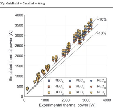
three correlations for the condensing ﬂow in the recuperator, namely the correlations proposed by Longo et al.[44], Han et al. [45]and Shah[46].

Regarding the air-cooled condenser, the following correlations are

evaluated:

•

the common correlation proposed by Gnielinski [47]for single-phaseﬂows in the horizontal tubes;

•

the general correlation proposed by Cavallini et al.[48]for con-densingﬂows in the condenser tubes;

•

two correlations for the airflow across the coil, i.e. the empirical laws proposed in[47]and the one proposed by Wang et al.[49] Fewer correlations are tested for the condenser because of the better characterizedflow occurring in the horizontal tubes. For the sake of conciseness, the equations constituting these heat transfer correlations are not presented here, but they can be found inAppendix B. Because of the multiple zones coexisting in the heat exchangers, different corre-lations must be coupled to simulate one component. As listed in Table 4, it results nine different models for the brazed plate heat ex-changers (i.e. the evaporator and the recuperator), and two models for the condenser. In order to assess their reliability, the different models presented inTable 4are evaluated in the exact same conditions as in the reference dataset and the heat transfer predicted by each model is confronted to the experimental observations.

In the case of the condenser, the two models investigated (i.e. the modelsCDAandCDB) demonstrate fairly good agreement with the ex-perimental data. As shown inFig. 4, both models properly predict the heat transfer and the modelling deviations are smaller than 10% (on average, the relative errors are 2.6% and 1.9% for the modelsCDAand

CDB respectively). Regarding the brazed plate heat exchangers, the modelling performance of the different correlations is significantly lower. For both the recuperator and the evaporator, it appears that all the models, in every case, highly overpredict the convective heat transfer coefficients in the BPHEXs. In the case of the recuperator, as depicted inFig. 5, the simulated heat transfers are on average over-predicted by 40% in comparison to the experimental data. Regarding the evaporator, the heat powers predicted by the models match Table 3

Operating ranges of the reference dataset.

Variable Min. Max. Unit

ṁhtf h, 910 990 [g/s] Thtf su h, , 88 120 [°C] Q̇ev 3.4 15 kW ṁhtf c, 0.15 1.45 [kg/s] Thtf su c, , 17 25 [°C] Q̇cd 2.9 13.3 kW ṁwf 16 70 [g/s] Pev 6.5 14.5 [bar abs.] Pcd 1.6 6.6 [bar abs.] Ẇnet 23 1170 [W] Q̇rec 0.13 3.3 [kW] ηnet ORC, 0.5 8 [%] Mwf tot, 26 (±0.5) 26 (±0.5) [kg] 0 0.5 1 Temperature [°C] 80 100 120 140

H

_h,l

= 350 W/(m².K)

H

_c,l

= 480 W/(m².K)

H

_c,tp

= 1000 W/(m².K)

H

_c,v

= 300 W/(m².K)

Set of coefficients #1 0 0.5 1 Temperature [°C] 80 100 120 140

H

_h,l

= 505 W/(m².K)

H

_c,l

= 800 W/(m².K)

H

_c,tp

= 1e+04 W/(m².K)

H

_c,v

= 50 W/(m².K)

Set of coefficients #2 Spatial fraction [-] 0 0.5 1 Temperature [°C] 80 100 120 140

H

_h,l

= 100 W/(m².K)

H

_c,l

= 2000 W/(m².K)

H

_c,tp

= 2000 W/(m².K)

H

_c,v

= 120W/(m².K)

Set of coefficients #3

Fig. 3. Thermal transfer in an evaporator with three different set of convective heat transfer coefficients (temperature profile vs. normalized length). The red and the blue lines correspond to the temperature profiles of the hot and the cold fluids, respectively. The thermal performance are identical (same heat transfers) but the spatial distribution of the different zones is totally different. (For interpretation of the references to color in this figure legend, the reader is referred to the web version of this article.)

(7)

relatively well the experimental measurements. Indeed, the heat ex-changer being slightly oversized for the tests conducted, a small pinch point is recorded experimentally for most of the points (i.e. lower than 3 K) while all the models predict a maximal heat transfer (i.e. with a pinch point equal to zero) whatever the operating conditions. However, the surface areas calculated for such zero-pinch heat transfers are much smaller than the eﬀective size of the evaporator. Therefore, the con-vective heat transfer coeﬃcients provided by the state-of-the-art cor-relations are also largely overestimated in the evaporator. Other studies (e.g.[50,51]) demonstrated similar results.

These poor predictions from the state-of-the-art correlations may be explained by different reasons. Firstly, the single-phase correlations are all empirically determined using water as heat transferfluid and their extrapolability to organicfluids is not verified. Secondly, even though the two-phase correlations are developed with refrigerants (or other organic fluids), the operating conditions used to calibrate them are more typical of refrigeration systems than those encountered in ORC units. In the case of condensingflows, the saturation temperatures in the two technologies (ORC and HVAC) are of the same order (20°C to more than 50 °C). However, the evaporating temperature in HVAC systems is much smaller than in ORC power units (−10 C/20 C vs.° °

° °

80 C/150 C). Therefore, the validity of the correlations to characterize boilingﬂows in ORC systems is not guaranteed. Finally, the correlations require a good knowledge of the BPHEX geometry (i.e. the chevron angle, the plate thickness, the enlargement factor, the corrugation pattern, etc.). Although some characteristics may be retrieved indirectly from the heat exchanger datasheet, uncertainties remain and these er-rors may alter the proper predictions of the correlations.

From these results, it appears that the correlations evaluated in this work (especially for the BPHEXs) cannot not be used directly to simu-late the investigated ORC system. However, the form of their equations is a good guess to compute the convective heat transfer coefficients. As a compromise, it is proposed to re-identify the empirical parameters of these correlations so as to betterfit the experimental measurements. To this end, three different identification methods, each giving an addi-tional degree of freedom, are applied for all the models given in Table 4, i.e.:

•

Method #1: only the most inﬂuential correlation in the heat ex-changer (i.e. the one referring to the highest thermal resistivity) is scaled by means of a single factor c, i.e.

=

Nunew c Nu· (2)

Table 4

Heat exchangers models investigated for the evaporator, the recuperator and the condenser (NB:(1)_{= Han’s boiling correlation}_[42]_;(2)_{= Han’s condensation correlation}_[45]_).

Evaporator models

(correlations for single-phase & boilingﬂows in a BPHEX)

EVA: Martin + Amalﬁ EVD: Martin + Han(1) EVG: Martin + Cooper

EVB: Wanniarachchi + Amalﬁ EVE: Wanniarachchi + Han(1) EVH: Wanniarachchi + Cooper

EVC: Thonon + Amalﬁ EVF: Thonon + Han(1) EVI: Thonon + Cooper

Recuperator models

(correlations for single-phase & condensingﬂows in a BPHEX)

RECA: Martin + Longo RECD: Martin + Han(2) RECG: Martin + Shah

RECB: Wanniarachchi + Longo RECE: Wanniarachchi + Han(2) RECH: Wanniarachchi + Shah

RECC: Thonon + Longo RECF: Thonon + Han(2) RECI: Thonon + Shah

Condenser models

(correlations for single-phase & condensingﬂows in tubes + air ﬂow through the coil) CDA: Gnielinski + Cavallini + VDI CDB: Gnielinski + Cavallini + Wang

Experimental thermal power [kW]

2 4 6 8 10 12 14

Simulated thermal power [kW]

2 4 6 8 10 12 14

CD

_A

CD

_B

-10%

+10%

Fig. 4. Parity plot of the condenser heat transfer (simulation results vs. experimental data).

Experimental thermal power [W]

0 1000 2000 3000 4000

Simulated thermal power [W]

0 500 1000 1500 2000 2500 3000 3500 4000 REC_A REC_B REC_C REC_D REC_E REC_F REC_G REC_H REC_I -10% +10%

Fig. 5. Parity plot of the recuperator heat transfer (simulation results vs. experimental data).

(8)

•

Method #2: idem as method #1, except that all the correlations used to simulate the heat exchanger are scaled with independent factors

cj, i.e. =

Nunew j, c Nuj· j (3)

Therefore, two (resp. three) scaling factors are tuned for each BPHEX (resp. FCHEX) model.

•

Method #3: idem as method#2, except that, additionally, the em-pirical exponents on the Reynolds number (m in Eq.(4)) are also tuned by factors ck, i.e.

=

Nunew jk, c Nu Rej· j( c mk· ) (4) In total, four (resp. six) factors are tuned for each BPHEX (resp. condenser) model.

For each model listed inTable 4, the scaling factorscjk are tuned by minimizing the residuals between the model predictions and the ex-perimental data. More speciﬁcally, the following objective function F is minimized by means of an interior-point algorithm[52], i.e.

∑

= + − − = F β NRMSE β c M min · (1 )· 1 c j M jk 1 jk ₍₅₎

where theﬁrst term is referring to the Normalized Root Mean Square Error (as deﬁned in Eq.(6)), the second term accounts for the correction applied to the correlations (aimed to be minimized as well) and β is a weighting factor (set to 0.95 in this work).

= − ∑₌ − NRMSE Q Q Q Q N 1 ̇ ̇ ( ̇ ̇ ) max min i N exp i sim i 1 , , 2 (6) In order to compare these methods, averaged values of the NRMSE related to each modelling approach are given inFig. 6. As expected, the larger the tuning applied to the correlations, the better theﬁtting of the experimental data. From these results, the method#3(i.e. the method changing the most the initial correlations) seems to be the best ap-proach to evaluate the heat transfer coeﬃcient. However, as demon-strated in the next subsection, the thermal prediction of the heat ex-changer models should not be used as only indicator to assess the models validity.

3.2. Inﬂuence of the void fraction

As already shown in Eq.(1), the mass of workingfluid enclosed in a heat exchanger can be computed as the sum of the masses included in each of the zone. In the case of a single-phase zone (either sub-cooled or superheated), the density of thefluid is totally defined by its thermodynamic state and the enclosed mass can be easily computed as

=

Msp V ρsp· sp (7)

whereVspis the zone volume andρspis a mean value of the single-phase fluid density. In the case of a two-phase mixture, the density is not only function of thefluid thermodynamic state (i.e. its pressure, temperature and quality), but it also depends on theflow pattern characterizing the liquid and the vapour phases. To account for this effect, the two-phase flowing mixture is characterized by a void fractionαrelated to thefluid quality x, i.e. = = + −

( )

α x A A _S ( ) 1 1 cs v cs x x ρ ρ , 1 v l (8)

whereAcs v, andAcsare respectively the vapourﬂow and the total ﬂow cross-sectional areas, ρvandρlare the saturated vapour and saturated liquid densities, and S is the slip (velocity) ratio between the vapour phase and the liquid phase (i.e.S=u uv/ l). Based on the void fractionα, the mass Mtpenclosed in a two-phase zone of length L and of cross

section areaAccan be calculated i.e.

∫

= + =

(

+ −

)

Mtp Mv Ml Ac ρv α x dl( ) ρ [1 α x dl( )] L l L 0 0 (9)

It is important to note that the void fraction in Eq.(9)is integrated along l, i.e. the length of the zone, whileαis expressed in terms of the fluid quality. To facilitate the calculation, a common approach is to assume a uniform heatflux in the two-phase zone[53]and thereby a linear evolution of thefluid quality along the length l. In this work, such an assumption is avoided and the effective spatial evolution of the quality in the heat exchanger is taken into account. To this end, the two-phase region is not evaluated as a single zone but it is further discretized into ten sub-cells. This approach is more computationally intensive, but it gains in modelling accuracy.

As for the heat transfer coefficients, many correlations may be found in the scientific literature to characterize the void fraction in function of the flow operating conditions [54]. In this work, five of the most commonly used void fraction models are considered, namely:

•

the homogenous model, which assumes a slip-ratio S equal to 1;

•

the model proposed by Zivi [55], which computes the slip-ratio accounting for the operating pressure such as_S=_{( / )}_{ρ ρ} −

v l 1/3;

•

the model proposed by Lockhart-Martinelli[56], which calculatesα

as an empirical function of the eponymous parameterXtt;

•

the empirical model proposed by Premoli[57]which accounts for the massﬂux in the void fraction calculation;

•

a second empirical mass-ﬂux-dependent model proposed by Hughmark[58].

As a ﬁgure of comparison, the inﬂuence of these void fraction models on the density calculation is depicted inFig. 7. The constitutive equations of these models can be found inAppendix B.

In order to compare thefive void fraction models, the mass of fluid enclosed in the three heat exchangers is computed for the 40 points constituting the reference dataset. Since there is no measurement of the individual charge in each heat exchanger, the reliability of the void fraction models is assessed by comparing the total charge prediction in the entire system to the effective mass of fluid enclosed in the ORC test rig (26 kg ± 0.5 kg). The total mass of fluid in the ORC is simply computed as the sum of the masses enclosed in the different compo-nents i.e.

∑

= + + + + + +

Mwf tot Mev Mrec Mcd MLR Mexp Mpp M i

pipe i

, ,

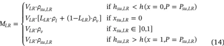
(10) where the masses in the expanderMexp, the pumpMpp, the liquid re-ceiver MLRand the various pipings Mpipeare computed using Eqs.(A.6),

(14) and (A.9). In order to numerically quantify the goodness of the charge predictions, both the mass mean value (i.e. the average mass computed over the 40 experimental points) and the mass standard de-viation (to illustrate the mass scattering) are computed for the diﬀerent modelling approaches. Because there are 2 models of the condenser, 9 models for the BPHEXs and 4 tuning methods, all independent from each other, 72 diﬀerent combinations of the HEXs models are tested to

REC EV CD Averaged NRMSE (-) 0 2 4 6 8 10 Original correlations Correlations with method #1 Correlations with method #2 Correlations with method #3

Fig. 6. Averaged values of the NRMSEs committed for each heat exchanger in function of the tuning method applied to the correlations.

(9)

simulate the ORC system (i.e. all the combinations possible are eval-uated). For each of these 72 model combinations, theﬁve void fractions are used to compute the total mass of workingﬂuid enclosed in the system. Ultimately, 360 charge-sensitive simulations are performed and all the detailed results can be found inAppendix C. For the sake of clarity, averaged values of the charge inventory are depicted inFig. 8. Out of this comparative study, the following elements can be high-lighted:

•

Regarding the condenser, the model CDB shows a slightly better thermal performance (i.e. itﬁts a little better the experimental data in terms of heat transfer in the condenser), but it induces much larger scattering in the global mass calculation (i.e. larger standard deviations of Mwf tot, ) whatever the identiﬁcation method employed

toﬁnd the convective coeﬃcients.

•

Regarding the evaporator and the recuperator, the type of correla-tions used to simulate the BPHEXs does not inﬂuence much the mass inventory calculation once an identiﬁcation method is applied to the original correlation. The models EVAandRECA(i.e. the ones based

on Martin’s, Amalﬁ’s and Longo’s correlations) demonstrate slightly better results.

•

In all situations, the homogenous and the Hughmark’s void fraction models lead to the lowest and the highest mass estimations, re-spectively. On average, the difference between their total mass predictions is 2.54 kg. On the other hand, the void fractions pro-posed by Zivi, Lockhart-Martinelli and Premoli lead to intermediate charge inventories. Whatever the identification method and the heat transfer correlations employed, Hughmark’s void fraction model (which accounts for the influence of the fluid mass flux) appears to be the best modelling approach. In every case, it leads to the lowest error in the prediction of the charge and to the lowest standard deviation.

•

The mass standard deviation is not much influenced by the void fraction model, but rather by the identification method applied to find the convective heat transfer coefficients. As shown in the pre-vious section, the larger the modifications applied to the original correlations, the better thefitting of the heat power transferred in the heat exchangers. However, as shown inFig. 8, the larger these modifications, the wider the scattering in the mass predictions. By altering the state-of-the-art correlations, the thermal performance of the heat exchanger models is improved but the charge inventory predictions are deteriorated.

Out of this study, it appears that the best modelling choices to si-mulate the heat exchangers is the void fraction proposed by Hughmark, the modelCDA for the condenser and the models EV RECA/ A for the brazed plate heat exchangers (cfrTable 4). Regarding the method used to identify the heat transfer coefficients, a trade-off must be made be-tween the thermal performance and the charge inventory predictions of the heat exchanger models. So far, it is unclear which criteria is the most important to perform charge-sensitive simulations of a ORC system. Indeed, it might be valuable to give more credit to one criteria over the other if its influence was demonstrated to be more important for the simulation of the closed-loop system. To assess this point, it is required to simulate the entire ORC power system and to confront the model predictions with the experimental data.

4. Other components modelling

In order to simulate the entire ORC power system, other models are required to characterize the rest of the components. The following section presents the models used to simulate the scroll expander, the

Quality x (-)

0 0.2 0.4 0.6 0.8 1

Density (kg/m3)

0 200 400 600 800 1000 1200

Homogenous

Zivi

Lockhart Martinelli

Premoli

Hughmark

Fig. 7. Density of R245fa as a function of the quality computed with 5 diﬀerent void fraction models (example conditions:_P=_{8 bar,}_D =_{3.2 mm,}_G=_{2.97 kg·s}−_·m

h 1 2).

Original

Method #1

Method #2

Method #3

Averaged

mean mass [kg]

15

20

25

30 Original

Method #1

Method #2

Method #3

Averaged

std deviation [kg]

0

2

4

Homogenous Zivi Lockhart Martinelli Premoli Hughmark

Experimental charge = 26 kg

Fig. 8. Averaged results of the global charge predictions (in terms of mean mass and standard deviation) in function of the void fraction model employed and the tuning method applied to the convective heat transfer correlations. Thisﬁgure summarizes the detailed results provided in Appendix C.

(10)

diaphragm pump, the pipings and the liquid receiver. 4.1. Mechanical devices

Both the pump and the expander are simulated with semi-empirical models. This kind of model relies on a limited number of meaningful equations that describe the most significant phenomena occurring in the process. Such a modelling approach offers a good compromise be-tween calibration efforts, simulation speed, modelling accuracy and extrapolation capabilities[11]. More specifically, the scroll expander is simulated by means of the grey-box model proposed by Lemort et al. [59]. Besides of under- and over-expansion losses (due to the fixed built-in volumetric ratio of the scroll expander), this model accounts for heat transfers and pressure drops at the inlet and outlet ports of the machine, mechanical losses, internal leakages and heat losses to the environment. The pump is modelled in a similar way with the model proposed in[60]. The pump model accounts for ambient losses, internal leakages, mechanical losses and cavitation phenomena (as proposed by Landelle et al.[61]).

For an extensive description of the models equations, please refer to the corresponding references. The parameters of these two semi-em-pirical models are calibrated to fit the experimental measurements. Regarding the charge modelling, the mass of workingfluid enclosed in the two mechanical components is simply computed assuming afluid mean density (Eq.(A.6)). The volumeVmecis computed as the sum of the swept and the discharge volumes of these machines (retrieved from the components datasheet). This simplified approach is justified by the relatively small internal volumes in the mechanical components.

4.2. Liquid receiver

The liquid receiver (LR) is a single tank placed at the condenser outlet and used as a buffer reservoir. As demonstrated below, its goal in normal conditions is to ensure a saturated liquid state at the condenser outlet and to damp mass transfer in off-design conditions. In this work, the modelling of the liquid receiver neglects heat losses to the en-vironment and hydrostatic effects due to the height of liquid (i.e. the pressure is assumed uniform through the liquid receiver). Therefore, the tank is thermodynamically passive for the working fluid and the equations used to model the liquid receiver are simply:

=

hsu LR, hex LR, (11)

=

Psu LR, Pex LR, (12)

The mass offluid stored in the reservoir is not straightforward to assess. Indeed, the level of liquid (defined as LLR=V Vl/ LR) varies in function of the operating conditions and directly influences the amount of refrigerant enclosed in the tank. In order to predict the level of liquid in the receiver, the model is based on the following hypotheses:

1. In stabilized regimes, the presence of a partial liquid level (i.e. ∈

LLR ]0,1[) imposes the enclosed ﬂuid to be in two-phase equili-brium.

2. Due to gravity and the absence of any entrainment eﬀect, saturated liquid lays at the bottom of the tank while vapour remains at the top.

3. If there is a liquid level, only a liquid phase can be extracted since the extraction port is placed at the bottom of the tank (dip tube, as depicted inFig. 9).

4. In steady-state conditions, the liquid level is constant and the mass balance implies an equality between the supply and the exhaust massﬂow rates, i.e.

=

ṁsu LR, ṁex LR, (13)

Although trivial individually, the combination of these four postu-lates leads to one important feature of the system: in steady-state op-eration (and in the absence of non-condensing gases), a liquid receiver may be a partiallyfilled (i.e.LLR∈]0,1[) only if a saturated liquid en-ters and leaves the reservoir. Indeed, if a sub-cooledfluid is supplied to the tank, a two-phase equilibrium cannot exist (cfr. postulate 1) and the liquid reservoir must be filled by sub-cooled fluid. If a superheated vapour enters the receiver, the same conclusion can be drawn. Finally, if a two-phase mixture enters the reservoir (e.g. with afluid quality

=

xsu LR, 0.2), a liquid-vapour equilibrium could exist. However, the exhaust port extracting a saturated liquid only (cfr. postulate 3), the receiver mass balance would be violated (since xex LR, =0). In order respect the fourth postulate, a liquid phase cannot reside in the tank and the reservoir must befilled of saturated vapour fluid. Based on this analysis, the mass of workingfluid in the receiver is calculated as fol-lows: = ⎧ ⎨ ⎪ ⎩ ⎪ < = = + − = ∈ > = = M V ρ h h x P P V L ρ L ρ x V ρ x V ρ h h x P P · if ( 0, ) ·[ · (1 )· ] if 0 · if ]0,1] · if ( 1, ) LR LR su LR su LR su LR LR LR l LR v su LR LR v su LR LR su LR su LR su LR , , , , , , , , ₍₁₄₎

whereLLR is the liquid level andρl (resp. ρv) is the saturated liquid (resp. vapour) density of thefluid at the supply pressure. It is important to note that under normal operating conditions, the receiver is intended to be partiallyfilled of liquid and it imposes a fluid subcooling of zero at the condenser outlet. In such conditions, the level of liquidLLRis given by the over amount of workingfluid that is not spread in the rest of the system. If the charge offluid is not properly chosen or if the ORC system is operating in strong off-design conditions, the receiver can be com-pletelyflooded or emptied. For a given operating pressure,Fig. 10 il-lustrates the mass of refrigerant enclosed in the liquid receiver as a function of thefluid supply enthalpy. It can be seen that a large dis-continuity in the mass profile occurs when the fluid reaches its satu-rated liquid state (i.e.xsu LR, =0). As further discussed in Section5, this discontinuity leads to numerical issues when modelling the entire ORC system. Finally, in the test rig investigated here, cavitation problems with the diaphragm pump imposed to voluntarily over-charge the system of workingfluid to ensure a minimum fluid subcooling. There-fore, most of the points included in the experimental dataset feature a flooded liquid receiver.

4.3. Piping

Besides the active components constituting the ORC system, pres-sure drops and heat losses induced by the interconnecting pipelines are also taken into account. These losses are lumped in the high- and the low-pressure lines by means of single artiﬁcial components placed at the outlet of the evaporator and the condenser, respectively. The

L

_LR

X

_su,LR

= 0

X

_ex,LR

= 0

(11)

pressure losses are computed as a linear function of the fluid kinetic energy (Eq.(A.7)) while ambient heat losses are modelled with a single empirical heat transfer coefficient (Eq.(A.8)) The mass of workingfluid enclosed in every section of interconnecting pipes is also taken into account (Eq.(A.9)).

5. ORC system modelling

The model of the entire ORC system is obtained by coupling in series the models describing each subcomponent. As depicted inFig. 11, the ORC model is built in such a way that the unit performance is derived

from its boundary conditions only. These boundary conditions are chosen to be exactly the same as seen in practice by the test rig, namely

•

the heat source supply conditions (Thtf h su, , ,Phtf h su, , , ̇mhtf h, );

•

the heat sink supply conditions (Thtf c su, , ,Phtf c su, , , ̇mhtf c,);

•

the ambient temperature;

•

the rotational speeds of the mechanical components (e.g. pump and expander);

•

the components geometry;

•

the total mass of refrigerant in the system;

Apart of these inputs and the parameters characterizing each com-ponent, the ORC model does not rely on any user-speciﬁed assumption in the cycle state (e.g. an imposed subcooling, superheating, massﬂow rate, operating pressure or temperatures, etc.).

Such modelling of a closed-loop system is highly implicit because of the multiple interactions between the workingfluid states, the different components performance and the system boundary conditions. Therefore, the thermodynamic state of the engine cannot be computed straightforwardly but it is found through an optimization aiming to drive internal modelling residuals to zero. More specifically, the ORC model iterates on the evaporator outlet enthalpy (it1=hev ex, ), the

eva-porating pressure (it2=Ppp ex, ), the condensing pressure (it3=Ppp su, ) and

the condenser outlet subcooling (it4=ΔTsc) in order to decrease the following residuals below a predeﬁned threshold (₁₀−6_):

= − res N N 1 exp exp 1 ,2 (15) = − res h h 1 cd ex cd ex 3 , ,2 , (16) = − res h h 1 ev ex ev ex 3 , ,2 , (17)

Supply enthalpy [kJ/kg]

150 200 250 300 350 400 450 500

R245fa mass [kg]

0 1 2 3 4 5 6 7 8 9 sub-cooled liquid saturated liquid two-phase mixture superheater vapour Liquid level = 100% Liquid level = 0%

Fig. 10. Mass enclosed in the liquid receiver as a function of theﬂuid supply enthalpy (for a supply pressure of 3 bar).

h

ev,ex2

P

_ev,ex

m

pp

m

_htf,c

T

_htf,c,su

P

_htf,c,su

m

_htf,h

T

_htf,h,su

P

htf,h,su Pexp,su Pexp,ex Pcd,su hcd,su m_htf,c mpp Phtf,c,su Thtf,c,su

h

ev,su

P

_ev,su

m

_pp

P

_recc,su Qcd Prech,su h_rech,su m_pp Pexp,ex hcd,ex

ΔT

sc

P

_pp,su

P

pp,ex

N

_pp Model

PP

N

_exp

N

_pp

M

_wf

MODELS PARAMETERS

(

EV

–

EXP

–

PP

–

CD

–

REC

–

Piping

)

m

wf

P

_wf,i

, T

_wf,i

, h

_wf,i

along the cycle

W

_i

, Q

_i

along the cycle

OUTPUTS

INPUTS

ORC model

EV

model

HP

Losses model

EXP

model

LP

Losses model

REC

model

P

_pp,ex

h

_ev,ex mpp hexp,su Nexp,2

P

_pp,su

ΔT

sc Wexp hcd,ex2 Pcd,ex

CD

model 1 2 3 4 5 7 6

h

recc,su

W

pp

m

_htf,h

P

_htf,h,su

T

_htf,h,su

m

pp

m

_pp

Q

_ev mpp

Mwf,2=Mpp+Mrech+Mev+ Mexp+ Mrecc+ Mcd+ MLR+ ∑iMpipes,i

8

T

_amb

Fig. 11. Solver architecture of the ORC model with the inputs depicted in blue, the outputs in brown, the parameters in green, the iteration variables in red and the model residuals in violet. The circled number in each subcomponent model informs the execution order of the model. (For interpretation of the references to color in thisﬁgure legend, the reader is referred to the web version of this article.)

(12)

= − res M M 1 wf wf tot 4 ,2 , (18)

For a better understanding of the sub-models interaction, the ar-chitecture of the ORC model is depicted in Fig. 11. When the ORC system features a liquid receiver, the numerical resolution of this 4-dimension problem is uneasy because of convergence issues. For in-creased robustness, a two-stage solver is developed to perform charge-sensitive simulations. A detailed description of this solver is presented inAppendix D

6. Model validation and discussion

In this section, the ORC model is validated by simulating the com-plete test rig in the exact same conditions as the 40 reference points of the experimental dataset. To this end, only the boundary conditions of the test rig are provided as inputs to the ORC model. The resulting state predicted for the entire system is then confronted to the experimental measurements. The ORC model is tested with the three identification methods investigated to calculate the convective heat transfer coeffi-cients in the HEXs (cfr. Section3). Furthermore, to emphasize the effect of imposing the charge in the ORC model instead of the fluid sub-cooling, the results of the charge-sensitive model are compared to the predictions obtained when the subcooling is imposed to 3 different values (i.e. the mean, the lowest and the highest subcooling reached experimentally, equal to 13 K, 4 K and 23 K respectively). For the sake of simplicity, the model outputs are only compared in terms of the system net thermal efficiency, i.e.

= − − η W W W Q ̇ ̇ ̇ ̇ net ORC exp pp cd ev , (19) whereẆppand Ẇcdare the pump and the condenser fan consumptions, Ẇexpis the expander power generation, and Q̇evis the heat transfer rate in the evaporator. The mean percent error committed by the different models when predicting this net thermal efficiency is depicted in Fig. 12. Out of thisfigure, the following conclusions may be derived:

•

A poor characterization of thefluid subcooling as a significant im-pact on the modelling of the ORC power system, especially if the subcooling is overpredicted. On average, an overestimation (resp. underestimation) of the subcooling of 1 K relatively decreases (resp. increases) the prediction of the ORC net thermal efficiency by 3%.

•

When thefluid subcooling is imposed, the more the original heat transfer correlations are changed (method#1→#3), the better the ORC model predictions. This observation is totally in accordance with the results presented in Section3.1since these identification methods increasingly better fit the heat transfer in the heat ex-changers.

•

When the total charge of workingfluid is imposed, however, the opposite trend is seen: the more the convective heat transfer coef-ficients are changed, the poorer the ORC model predictions. For the system net thermal efficiency, the mean percent error committed by the ORC model when using the identification methods #1, #2 and #3 is equal to 11.6%, 28.8% and 44.2% respectively. According to the results shown in Section3.1, such high residuals are due to an improper modelling of the mass enclosed in the various heat ex-changers. Consequently, it can be concluded that a proper estima-tion of the mass enclosed in the heat exchangers is much more im-portant that a slight gain in the heat transfer predictions.

Based on these results, one may think that if thefluid subcooling was well known (e.g.ΔTscwould not change in function of the operating conditions and could be imposed in the ORC model), the best identifi-cation method would be the #3 since it shows the lowest residuals. This conclusion is wrong. Indeed, the results inFig. 12only illustrate the ability of the ORC models tofit a dataset while their true purpose is to

reliably predict the system performance in unseen conditions. The charge-sensitive results (in which the mass is imposed instead of the subcooling) show that the convective heat transfer coefficients given by the methods #2 and #3 do not predict properly the zones distribution in the heat exchangers. Since these coefficients fail to replicate the phenomena occurring inside the heat exchangers, the extrapolability of these HEX models (and, by extension, of the ORC model too) is not guaranteed. As mentioned in Section 3.1, the modelling of the heat exchangers is somehow problematic because different combinations of convective heat transfer coefficients may lead to similar heat transfer predictions. As demonstrated here, the modelling of the charge provides a new criteria to better assess the reliability of the convective heat transfer coefficients used to describe the heat exchangers. Taking the charge into account helps to reduce overfitting issues.

The most suited identification method to be applied to the state-of-the-art correlations is the method #1. By only scaling one heat transfer correlation (the one referring to the highest thermal resistivity in the heat transfer), this tuning method efficiently improves the thermal predictions in the heat exchanger model while ensuring a proper mass evaluation in the ORC system. For the case study investigated here, the parameters used to simulate the heat exchangers are summarized in Table 5. Additionally, parity plots of some key model outputs are de-picted inFig. 13. It can be seen that the ORC model predicts well the thermal power transferred in the heat exchangers with a mean percent error lower than 2%. Regarding the mechanical powers of the pump and the expander, larger deviations are observed (mean percent error < 11.5%) because of the higher sensitivity to deviations in the cycle pressures. However, the points showing the largest deviations are also the most sensitive to the uncertainty in the total charge of working fluid (known to be 26 kg ± 0.5 kg). Finally, the mean percent error committed on net thermal efficiency prediction is 11.6%. Considering the accumulation of errors and the absence of any intrinsic assumption in the system state to compute this efficiency, such an error is found acceptable. This charge-sensitive model can therefore be used to re-liably predict the ORC system behaviour in off-design conditions based on its boundary conditions only.

7. Conclusion

The present work focuses on the development and the validation of a charge-sensitive ORC model to be used for oﬀ-design performance simulations. A 2 kWe recuperative ORC unit is used as case study and experimental data are exploited to validate the models. The goal is to

Method #1 Method #2 Method #3

Mean error

net,ORC

(%)

0 10 20 30 40 50

T

_sc

= T

_sc,mean

T

_sc

= T

_sc,min

T

_sc

= T

_sc,max

M

_ORC

= 26 kg

Fig. 12. Mean Absolute Percent Error (MAPE) committed on the net ORC eﬃciency in function of the identiﬁcation method applied to simulate the HEXs and the subcooling/ mass imposed in the ORC model.

(13)

develop a reliable model which only accounts for the system boundary conditions (i.e. the heat source/heat sink supply conditions, the me-chanical components rotational speeds, the ambient temperature and the total charge of workingfluid) to predict the ORC system perfor-mance. To this end, models are developed to characterize each sub-components and they are assembled to simulate the entire closed-loop system. The heat exchanger modelling is investigated in detail and three different methods are tested to calculate the convective heat transfer coefficients. Out of this study, the main outcomes can be summarized as follows:

•

For performing charge-sensitive simulations, it is mandatory to properly predict the mass of ﬂuid enclosed in the various heat

exchangers. If several zones offluid co-exist in a same component, this implies a good modelling of the spatial distribution occupied by the different zones. The identification of the convective heat transfer coefficients (which directly impact the zones distribution) is uneasy without dedicated experiments and state-of-the-art correlations should be used as initial guesses.

•

Among nine different convective heat transfer correlations, the single-phase correlation of Martin[38], the condensing correlation of Longo et al.[44]and the boiling correlation of Amalfi et al.[41] are shown to be good candidates for characterizing the BPHEXs. Regarding thefin coil condenser, the air-side heat transfer correla-tion given in[47]is the best option. However, these correlations should only be considered as initial guesses to calculate the effective convective heat transfer coefficients. In order to better represent the thermal performance of the HEXs, the correlations parameters can be re-tuned by means of an identification method (mandatory in this case for the BPHEXs).

•

When re-identifying the parameters of the convective heat transfer correlations, the heat transfer predictions of the HEX models are improved but the charge inventory of the global system is deterio-rated.

•

Among the three identification methods investigated for the case study, the least intrusive (i.e. method #1) is the best to retrieve the convective heat transfer coefficients in the heat exchangers. By only scaling one convective heat transfer coefficient (the one referring to the highest thermal resistivity in the heat transfer), this identi fica-tion method efficiently fits the thermal performance of the heat exchangers while ensuring a proper global charge estimation in the ORC system. Furthermore, when modelling the entire ORC system, it is shown that a proper estimation of the mass enclosed in the heat exchangers is more important than a slight improvement of the heat transfer predictions.

Table 5

Parameters of the charge-sensitive HEX models.

Evaporator

Single-phase correlation: Martin (withc=0.268) Boiling correlation: Amalﬁ et al. (unchanged)

Void fraction: Hughmark

Recuperator

Single-phase correlation: Martin (withc=0.6557) Condensation correlation: Longo et al. (unchanged)

Condenser

Air-side correlation: VDI (withc=0.896) Single-phase correlation: Gnielinski (unchanged) Condensation correlation: Cavallini et al. (unchanged)

Experimental data 0 5 10 15 Simulation results 0 5 10 15 + 0.05 % - 0.05 % Experimental data 0 5 10 15 Simulation results 0 5 10 15 + 0.05 % - 0.05 % Experimental data 0 0.5 1 1.5 Simulation results 0 0.5 1 1.5 + 0.15 % - 0.15 % Experimental data 0 0.06 0.12 0.18 Simulation results 0 0.06 0.12 0.18 + 0.15 % - 0.15 % Experimental data 0 3 6 9 Simulation results 0 3 6 9 + 0.15 % - 0.15 % Experimental data 0 0.03 0.06 0.09 Simulation results 0 0.03 0.06 0.09 + 0.05 % - 0.05 %

Fig. 13. Parity plots between the experimental data (x-axis) and the simulation results (y-axis) predicted by the charge-sensitive ORC model using the identiﬁcation method #1 and with a total charge of 26 kg (the vertical bars account for the ±0.5 kg uncertainty of the experimental charge).