Opportunistic localization scheme based on linear matrix inequality

Open Archive Toulouse Archive Ouverte (OATAO)

OATAO is an open access repository that collects the work of Toulouse researchers

and makes it freely available over the web where possible.

This is an author-deposited version published in: http://oatao.univ-toulouse.fr/

Eprints ID: 2582

To cite this version: ZORZI, Francesco. KANG, GuoDong.

PÉRENNOU, Tanguy. ZANELLA, Andrea. Opportunistic localization

scheme based on linear matrix inequality. In: NEWCOM++ - ACoRN

Joint Workshop, 01 April 2009, Barcelona, Spain.

Any correspondence concerning this service should be sent to the repository

administrator:

[email protected]

OPPORTUNISTIC LOCALIZATION SCHEME BASED ON LINEAR MATRIX

INEQUALITY

Francesco Zorzi

_{, GuoDong Kang}

_{, Tanguy Pérennou}

_{and Andrea Zanella}

†_{Dept of Information Engineering, University of Padova}

e-mail: {zorzifra, zanella}@dei.unipd.it

‡_{CNRS ; LAAS ; ISAE ; Université de Toulouse}

e-mail: {gkang, perennou}@isae.fr

ABSTRACT

Localization and Tracking are very interesting functionalities that can benefit a number of applications. Despite the large num-ber of algorithms and technologies that have been proposed in this context, the literature still lacks a widely accepted solution, capa-ble of cutting a tradeoff between service quality (i.e., localization accuracy) and device/architecture cost and complexity. In this pa-per, we tackle the problem from a different and rather new perspec-tive: we investigate how the localization accuracy of nodes can be ameliorated by opportunistically exchanging localization informa-tion among nodes that occasionally happen to be in proximity. To this end, we define a simple though accurate model of the opportuni-stic interaction and we develop a technique based on Linear Matrix Inequalities and barycentric algorithm in order to localize a user node that is completely unaware of its position. We analyse the opportunistic localization performance for different settings of the design parameters as duty–cycle and error modeling taking into ac-count accuracy, degradation in time, correlation among consecutive estimation.

1. INTRODUCTION

Localization and Tracking are very interesting problems that have been deeply studied in several different contexts, from robotics to telecommunications systems, thanks to the large set of possibilities and optimizations that might be enabled by knowing the geographi-cal position of the nodes in a communication system. The accuracy of the localization estimation is strictly related to the environment and the technology used by the devices to localize themselves. A cheap and widespread technology like the Received Signal Strength Indicator (RSSI) is very poor for localization, while more expensive hardware can achieve better performance, for instance by compar-ing the Time of Arrival of radio signals or uscompar-ing acoustic or opti-cal signals. Other very specific solutions are proposed as Ekahau [1], ActiveBadge [2], Pseudolites [3], but they require very specific hardware and very complex infrastructure.

Whereas most of the solutions proposed in the literature are fo-cused on specific scenarios (static or dynamic, indoor or outdoor) with homogeneous devices, an emerging research trend aims at im-proving the localization accuracy by exploiting the device hetero-geneity through cooperative strategies. The scenario considered in most of such works encompasses teams of mobile autonomous robots equipped with different sensors that can cooperate one an-other and, occasionally, interact with simple sensors placed in the environment to achieve a given target, such as node localization and tracking. In this type of systems, cooperation is usually realized in a systematic way, i.e., the system is designed in order to facil-itate nodes cooperation. Conversely, when nodes actions are not bounded to a cooperative scheme, but cooperation is still enabled on an occasional basis, then we shall better talk of opportunistic interaction.

This work was partly supported by the European Commission in the framework of the FP7 Network of Excellence in Wireless COMmunications NEWCOM++ (contract n. 216715) and by French ANR Telecoms Project FIL.

Such a vision offers a number of research challenges, such as the definition of efficient nodes discovery and link establishment algorithms for opportunistic data exchange between multi-interface devices, the design of suitable opportunistic data exchange proto-cols, the devising of localization enhancing schemes based on op-portunistic data exchange, the investigation of the tradeoffs between different performance indexes (such as, localization accuracy versus protocol overhead/channel occupancy/energy consumption).

Affording these challenges all together would result in a over-whelming task. Therefore, we prefer to decouple the different as-pects and focus on a subset of the open problems.

More specifically, we propose a simple (but realistic) model for opportunistic information exchange that takes into account some important design parameters, such as the coverage range, the fre-quency of scan/query phases by which nodes look for opportunistic interactions and the amount of time dedicated to such a process.

2. RELATED WORK

Self-localization problem has been investigated in a number of pa-pers. Most common localization methods consist in measuring the power of the received RF signal (RSSI), the Time of Arrival (ToA) or the Angle of Arrival (AoA) of the RF signals from the beacons. In this way, every node estimates a set of distances from the beacons and, then, guesses its position by means of lateration and triangu-lation techniques [4, 5] or by using statistical estimation methods [6]. Overview of localization techniques based on RSSI and ToA measurements can be found in [7, 8, 9]. Multi-step localization techniques which involve refinement phase have been proposed by Savarese [10] and Savvides [5]. Other solutions need very special-ized hardware and a lot of complexity for the infrastructure as in [3, 2, 1].

In order to obtain good performance, a lot of complexity is needed, either in the infrastructure that in additional hardware to plug on low–cost nodes.

If mobility is added to the stray nodes, then the problem is to track it. This scenario is mainly applied on robots or mobile WSN. A lot of tracking algorithm are proposed, using Extended Kalman Filter as in [11] or Particle Filter as in [12], and [13], in order to exploit the correlation among different measurements.

If mobile nodes or robots can detect each other, they can use this information to refine their positions estimate. Cooperation scenario is studied very well in robotics. Many different techniques are pro-posed to exploit in the best way this information. In [14] the authors utilizes Markov localization for self–localize nodes and then proba-bilistic methods to synchronize each robot’s estimates when two of them have a contact. A distributed Kalman Filter is performed for collective localization in [15], avoiding a centralized data fusion, that is not so feasible in a cooperative scenario. An anchor-free ap-proach is then proposed in [16], where robots infer their position estimate only using the information exchanged among them.

Other similar frameworks are proposed for very specific appli-cations. In [17], the goal is localizing some video sensors used for surveillance applications. The measurements are the different angu-lar positions of a common object as seen by the different cameras. This information is then processed to determine their relative posi-tions.

In [18], a framework for autonomous vehicles in mining is pre-sented. Localization estimate of the mobile vehicle is provided by a primary localization system based on on-board odometry. To im-prove accuracy, some specific locations as, for example, gallery in-tersections, which can be easily recognized, are marked as land-marks.

In [19], an advanced integration of 802.11b equipments and In-ertial Navigation System (INS) is used to enhance the performance of the indoor positioning system. As a result, a system performance close to the meter accuracy can be achieved with a low density of access points in the environment provided that users carry inexpen-sive INS equipment.

3. MODELING

As mentioned, in this work we prefer to consider a simple, though significative, scenario that permits a first performance analysis of the opportunistic localization. Along these lines, we here introduce the assumptions that define our model that refers to the main idea in [20] for the opportunistic exchange and for error model.

Definitions and problem statement

We consider a system made of mobile Nodes equipped with a regu-lar communication device such as WiFi, Bluetooth or ZigBee. We then consider two kinds of nodes: User that is not capable of self-localization and Peer nodes that can estimate their position in time. A given peer i can therefore maintain a list of past position esti-mates that we define self-positioning estimations. The problem we address is how self-positioning estimations of Peers can be used by User to estimate its own position.

This problem can be expressed as a Linear Matrix Inequalities problem if we consider the communication range of each peer. At time t, user can exploit peer #i self-positioning estimation bPi(t) of

Peers that are within the coverage range R of the User. Let Pi(t) be

the exact position of the peer, ebi(t) an upper bound on the error

between exact and estimated positions, and Pu(t) be the exact

posi-tion of the user. This is a triangular inequality and For each peer #i within range of the user at time t we have the triangular inequality: ||Pu(t) − bPi(t)|| ≤ Ri+ ebi(t) (1)

Communication model

We focus on a single couple of nodes, say A and B, both equipped with a common wireless communication interface that is used for (opportunistic) data exchange. Radio propagation is described by means of a simple unit-disk model, according to which the radio transmission is always correctly received within a distance R

(cover-age range) from the transmitter, whereas it is not received at longer

distances. Although the unit-circle model is known to be oversim-plified, it permits to isolate the performance analysis from the char-acteristics of the radio interface that, at this stage of the work, is left generic. (In any case, the mathematical framework derived in the following section can be easily adapted to include more sophis-ticated radio-propagation models.)

Opportunistic interaction model

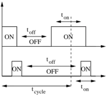
We assume that opportunistic interaction can actually occur only when both nodes are in the so-called Scan Phase, which may corre-spond to an interlaced Inquiry/Scan phase of Bluetooth or to the Ac-tive Scanning procedure of IEEE 802.11 systems. The scan phase is repeated with period T , asynchronously and independently by each node, so that the offset between the scan phases of two nodes can be modeled as a random variable with uniform distribution in the interval(0, T ). The duration of the scan phase, normalized to the scan period T , is called duty cycle and denoted byδ. Whereas the scan period T is the same for all the nodes, we suppose that each node can fix its own duty cycle depending on the requirements and the management policy of that node. Fig. 1 shows an example of the scan periods of A and B.

OFF ON ON ON _OFF ON t_off t_on off t cycle t t_on

Figure 1: Scan period

We suppose that opportunistic data exchange can occur (in a negligible time) only when the scan phases of the two nodes over-lap in time. Furthermore opportunistic data exchange also requires the nodes to be mutually in range. We assume that opportunistic interaction immediately takes place as soon as both conditions are satisfied. Such an event is coined rendez-vous.

Self-positioning model used by peers

We assume that peer nodes have “native” self-positioning capabil-ities, provided by some (non opportunistic) scheme. Accordingly, we denote by Piand bPithe real and the self-estimated position of

peer #i, expressed in polar coordinates. Peers can be classified in different classes, depending on their native self-localization accu-racy. For simplicity, we assume that the estimation error ei= Pi− bPi

can be modeled as the module of a 2–dimensional Gaussian random variable with zero mean and varianceσ2_{, which depends on the}

lo-calization class and for simplicity we assume to be the same for all nodes. Moreover, the error model considers two possible charac-teristics: correlation among consecutive estimations (considering a tracking-based technique) and degradation of the estimate in time, so that the positioning error is better modeled as a stochastic process

ei(t), with the following characterization:

• At the time t = 0, the positioning error ei(0) is the module of

a zero mean 2–D Gaussian Random Variable[x(0) y(0)], with standard deviationσ(0)

• At the time t > 0, ei(t) is drawn from the correlated Gaussian

distribution of the two coordinates:

fx(t)|x(t−1)(x(t)∗|x(t−1)∗;ρ)= exp " −(x(t)∗)2−2ρx(t)∗x(t−1)∗+(x(t−1)∗)2) 2(1−ρ2 ) # 2πσ(t)σ(t−1)√1−ρ2 (2) with x(t)∗₌ x(t) σ(t) and x(t − 1)∗= x(t−1) σ(t−1),ρ is the correlation coefficient chosen in the interval[0, 1], with 0 that means inde-pendent and 1 completely correlated samples.

The accuracy can degrade following the equation σ(t) =

σ(0) +αt, whereαis the drift of the estimation error.

During a rendez-vous, peer nodes send packets containing their estimated positions ˆPiand the class of accuracyσ2(t), that affects

the ebi(t) used in the LMI algorithm.

Self-positioning model used by the user

User node is not equipped with a self-positioning system and hence resorts to opportunistic localization to infer its geographical posi-tion. He stops and stays at a fixed position during the whole self-positioning process. Let W be this waiting duration measured as a number of scan periods starting at period t= 1. The user’s self-positioning estimations are then generated in two stages:

1. At every scan period t≥ 1, the user collects self-positioning estimations from peers that are within range and whose duty cycles overlap the user’s duty cycle. These estimations are used to solve the LMI system of equations 1. The resulting optimum

Figure 2: Raw LMI-only estimation

Figure 3: LMI+barycentric estimation

is used as a raw estimation dPu,r(t) of the user position. Fig. 2 shows how dPu,r(t) is generated at cycle t, assuming that only P1

and P2are within the user’s range at time t.

2. When t> 1, the user can compute the barycenter of the primary estimations computed since t= 1. We define this barycenter as the self-positioning estimation of the user at time t:

b Pu(t) = 1 t t

∑

This second stage is illustrated in Fig. 3, which shows how b

Pu(1), bPu(2) and bPu(3) are generated from dPu,r(t), t = 1, 2, 3. We have made numerous experiments with this model, and ob-served that in most cases, the self-positioning estimation improves over time. We therefore use the estimation only after a warm-up time denoted wu and measured in scan periods starting at t= 1.

4. SIMULATION RESULTS

The models described in the previous section have been imple-mented using Matlab R2008b and its Robust Control Toolbox which provides an LMI solver. In this section we define a reference test case and study the impact of selected parameters, here the duty cy-cleδ, the accuracy parameterσ(t) and the correlation parameterρ. The impact of other parameters such as the number of peers within range, the range itself and the speed of peer nodes has been studied in another paper [21] and will be briefly summed up.

4.1 Measuring accuracy

The performance of the user’s self-positioning estimation is natu-rally based on the measure of the distance between real and estimate position:_||Pu− bPu(t)||. However, as stated in Section 3, the

estima-tion becomes reliable after the warm-up time. Let wu be the number of scan periods of the warm-up and W the number of scan periods during which the user stays in the same position and collects data from peer. Then, we define the accuracy of an experiment as

A= 1 W− wu W

∑

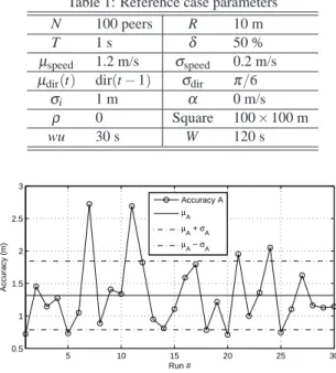
Our reference case involves N= 100 peer nodes moving in a 100 m × 100 m square and one user node remaining at the center of this square. Peers and user share the same radio range R= 10 meters, so that only a fraction of Peers are within range of the user at each time.

Peers and user also have the same scan period T = 1 second and the same duty cycleδ= 50%, so that duty cycles are always

Table 1: Reference case parameters

N 100 peers R 10 m

T 1 s δ 50 %

µspeed 1.2 m/s σspeed 0.2 m/s

µdir(t) dir(t − 1) σdir π/6

σi 1 m α 0 m/s ρ 0 Square 100× 100 m wu 30 s W 120 s 5 10 15 20 25 30 0.5 1 1.5 2 2.5 3 Run # Accuracy (m) Accuracy A µ_A µ_A + σ_A µ_A − σ_A

Figure 4: Reference case runs

partially overlapped. The scan period of the user starts at t= 0 while the scan period of each peer starts with an offset uniformly distributed in(0, T ).

The self-positioning estimations of each peer are generated as follows. First, the trajectory is computed using the Random Pedes-trian Mobility Model defined in [21]: this model is inspired by the Brownian movement, modified so that speeds are drawn from a Gaussian distribution N(1.2, 0.2) and at each time step the next direction is chosen in front of the pedestrian, i.e. in another Gaus-sian distribution centered on the previous direction, with a small standard deviation arbitrarily set toσdir=π/6. The trajectory is

kept within the considered square area. Second, for each position a self-estimation is produced using the peer self-positioning model defined in Section 3. In the reference case, the accuracy class of each peer has been set toσ = 1 meter and it is assumed constant over time, i.e. α= 0 m/s. Furthermore, the self-positioning esti-mates are not correlated, i.e. ρ = 0. In practice, each peer self-position estimation at cycle t is randomly drawn in a disc centered around the exact position of the peer at cycle t, using a 2D Gaussian distribution. Different settings for the self-positioning model will be tried later in this section.

Finally the user, placed in the center of the area, estimates its position using the opportunistic localization model defined in Sec-tion 3. The waiting time of the user is set to W = 2 minutes and the warm-up time is set to wu= 30 seconds. We will also see what happens for shorter and longer waiting times.

Table 1 sums up the parameter values used for the reference case.

Accuracy of the reference case

The reference case has been run 30 times with different random seeds. The results, in terms of localization error of the user node, strongly differ from one run to the other, as illustrated by Fig. 4. The mean of the accuracy over 30 runs isµA= 1.32 m and the standard

deviation isσA= 0.53 m, while the worst case has an accuracy of

2.72 m.

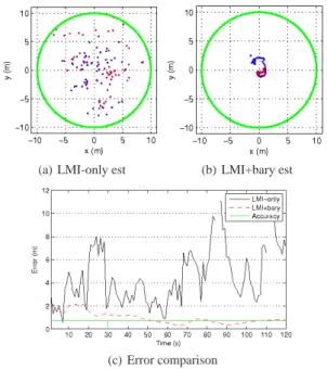
To better understand the behavior of the protocol, we report in Fig. 5(a) the successive user’s raw LMI estimations for a single run and in Fig. 5(b) the self-localization estimations of the user using LMI and barycenter algorithm. In both figures, the oldest plots are in blue and gradually turn to red. The barycentric estimation clearly

(a) LMI-only est (b) LMI+bary est

(c) Error comparison

Figure 5: Reference case run #1/30.

Table 2: Duty cycle impact

δ µA σA retained

20 % 2.51 m 1.20 m 1.13 peers 40 % 1.71 m 0.63 m 2.38 peers

50 % 1.32 m 0.53 m 3.01 peers

improves over time, and is better than the raw one. This is even remarked in Fig. 5(c), where the reader can compare the evolution of the raw error||Pu− dPu,r(t)|| and the error of the barycentric ap-proach||Pu− bPu(t)||. The run-wide accuracy A is also plotted.

In most runs, the accuracy of the barycentric estimation tends to improve over time: each additional raw LMI estimation contributes to improve the estimation, since new information is added.

4.3 Duty cycle impact

In this section we measure the impact of the duty cycle length. There is clearly a trade-off to find between rendezvous probability (long duty cycle) and energy consumption (short duty cycle). We have run the simulation 30 times for two additional values of duty cycleδ: 20 % and 40 %, the other parameters being the same as for the reference case above. The results are summed up in Table 2, where the last line is a reminder of the test case.

As expected, accuracy improves when the duty cycle increases thanks to the higher number of peer self-positioning estimations that improves the performance of the raw LMI location estimation scheme, and in turn the barycentric estimation.

4.4 Peers self-positioning impact

In this section we measure the impact of the self-positioning model characterizing peers. To this end, we consider three different pa-rameters: first, the correlation coefficientρ among successive self-positioning estimations of each peer; second, the self-self-positioning accuracy classσ of peers; third, the accuracy driftαof peers. The other parameters are set to the values of the reference case.

Table 3 gathers all the results. As it can be observed, the pa-rameters have negligible impact on the accuracy of the opportuni-stic localization scheme that, hence, proves to be rather robust to localization errors of Peers. This is likely due to the fact that, de-spite the errors, the positions provided by the Peers form a uniform

Table 3: Correlation impact

ρ σi α µA σA 0 1 m 0 m/s 1.32 m 0.53 m 0.4 1 m 0 m/s 1.32 m 0.53 m 0.9 1 m 0 m/s 1.31 m 0.55 m 0.99 1 m 0 m/s 1.33 m 0.55 m 0 3 m 0 m/s 1.36 m 0.56 m 0 5 m 0 m/s 1.43 m 0.61 m 0 1 m 0.01 m/s 1.32 m 0.53 m 0 1 m 0.03 m/s 1.33 m 0.53 m

“cloud” of points around the User. Then, applying the barycentric scheme, the User always localizes itself near the center of such a cloud. To verify this conjecture, however, we plan to consider in future work other error models for peers estimation, such as model for podometers, or for MEMS-based inertial navigation systems, or for RSS-based landmarks.

4.5 Other parameters

In a previous paper [21], we also studied the impact of other pa-rameters; we showed that the accuracy of the user self-positioning scheme degrades when: the amount of peers within range (N) de-creases, the range threshold R increases or the peers mean speed

µspeed decreases. We re-evaluate these parameters and others

quickly here.

For the setup used here, using 50 peers give a mean accuracy of 1.96 m while 200 peers give a mean accuracy of 0.84 m (this is not as overcrowded as it may seem, if you think of a station, a big mall or a conference room for instance: in a 100×100 square, this gives 50 m2_{per peer). Of course, the more peers there are with random}

trajectories, the more communication opportunities there are, and the more information are fed to the LMI system, which induces better estimations.

Another way to improve the accuracy is to increase the waiting time of the user: 5 minutes lead to an accuracy of 0.98 m. In that case, the barycentric estimation takes into account more and more raw LMI estimations, thus giving less weight to bad raw estima-tions. On the contrary, reducing to 1 minute degrades the accuracy to 1.92 m.

We also changed the range. A 5 m range leads to an accuracy of 1.07 m, while a 20 m range leads to an accuracy of 1.88 m. This is not an intuitive result, since a larger range would mean more oppor-tunities of sharing information. However, these additional positions are more far away from the user, which increase both the raw LMI error and the barycentric error.

Finally, we also changed the mean peer speed. If peers are slow (0.6 m/s) the accuracy degrades to 2.12 m. If peers are fast (3 m/s) the accuracy improves to 0.71 m.

5. CONCLUSION AND FUTURE WORKS

In this paper, we propose an algorithm in which a still user in-fers localization information using the positions of other passing-by nodes. The opportunistic interaction is modeled passing-by considering several parameters that permit to compare the performance of the scheme in different scenarios.

In all the cases considered in this study, we obtained a

local-ization error lower than 2.5 meters that can be reduced to less than

1 meter with an accurate tuning of the system parameters. In

par-ticular, the duty cycle of the opportunistic-scan phase has been ob-served to have a significant impact on the user self-positioning es-timation: the shorter the duty cycle the less the rendezvous prob-ability with peers and, in turn, the lower the localization accuracy. Furthermore, we observed that the proposed opportunistic localiza-tion scheme is rather robust to the self-posilocaliza-tioning error model for Peers. In fact, the correlation, the standard deviation and the drift of

the self-positioning error do not significantly affect the localization accuracy, provided that the algorithm is performed over the data gathered with a large enough number of opportunistic exchanges.

In order to complete this work, some improvements will be done. We will try to define a more realistic set-up involving dif-ferent types of peer nodes, e.g. access points with well-known po-sitions but only partial coverage and mobile peers carrying cheap INS systems which accuracy drifts over time. We will also imple-ment the opportunistic meeting model defined in [20] that applies to peer meetings. It is also possible to take into account different self-localization models and opportunistic update.

Acknowledgment

The authors would like to thank Yves Caumel from ISAE for his very valuable advices on interpretation of random behaviors.

REFERENCES

[1] I. Ekahau. [Online]. Available: http://www.ekahau.com/ [2] R. Want, A. Hopper, V. Falcao, and J. Gibbons, “The active

badge location system,” ACM Trans. Inf. Syst., vol. 10, no. 1, pp. 91–102, 1992.

[3] H. S. Cobb, “Gps pseudolites: theory, design, and applica-tions,” in Ph.D. Thesis - Stanford University, September 1997. [4] A. Savvides, H. Park, and M. B. Srivastava, “The n-hop mul-tilateration primitive for node localization problems,” Mobile

Network Applicatons, vol. 8, no. 4, pp. 443–451, 2003.

[5] A. Savvides, H. Park, and M. Srivastava, “The bits and flops of the n-hop multilateration primitive for node localization prob-lems,” 2002.

[6] N. Patwari, R. O’Dea, and Y. Wang, “Relative location in wireless networks,” in Proceedings of IEEE Veh. Tech. Conf.

(VTC), Rhodes, Greece.

[7] N. Patwari, J. N. Ash, S. Kyperountas, A. O. Hero III, R. L. Moses, and N. S. Correal, “Locating the nodes: cooperative localization in wireless sensor networks,” Signal Processing

Magazine, IEEE, vol. 22, no. 4, pp. 54–69, July 2005.

[8] A. Savvides, M. Srivastava, L. Girod, and D. Estrin, “Local-ization in sensor networks,” pp. 327–349, 2004.

[9] R. Huang and G. V. Zaruba, “Static path planning for mobile beacons to localize sensor networks,” Pervasive Computing

and Communications Workshops, 2007. PerCom Workshops ’07. Fifth Annual IEEE International Conference on, pp. 323–

330, March 2007.

[10] C. Savarese, J. Rabay, and K. Langendoen, “Robust position-ing algorithms for distributed ad-hoc wireless sensor networks usenix technical annual conference,” 2002.

[11] J. Leonard and H. Durrant-Whyte, “Mobile robot localization by tracking geometric beacons,” Robotics and Automation,

IEEE Transactions on, vol. 7, no. 3, pp. 376–382, Jun 1991.

[12] F. Dellaert, D. Fox, W. Burgard, and S. Thrun, “Monte carlo localization for mobile robots,” Robotics and Automation,

1999. Proceedings. 1999 IEEE International Conference on,

vol. 2, pp. 1322–1328 vol.2, 1999.

[13] D. Fox, W. Burgard, F. Dellaert, and S. Thrun, “Monte carlo localization: efficient position estimation for mobile robots,” in AAAI ’99/IAAI ’99: Proceedings of the sixteenth national

conference on Artificial intelligence and the eleventh Innova-tive applications of artificial intelligence conference. Menlo Park, CA, USA: American Association for Artificial Intelli-gence, 1999, pp. 343–349.

[14] D. Fox, W. Burgard, H. Kruppa, and S. Thrun, “A probabilis-tic approach to collaborative multi-robot localization,”

Au-tonomous Robots, vol. 8, June 2000.

[15] S. Roumeliotis and G. Bekey, “Collective localization: a dis-tributed kalman filter approach to localization of groups of

mobile robots,” Robotics and Automation, 2000.

Proceed-ings. ICRA ’00. IEEE International Conference on, vol. 3, pp.

2958–2965 vol.3, 2000.

[16] A. Howard, M. Matark, and G. Sukhatme, “Localization for mobile robot teams using maximum likelihood estimation,”

Intelligent Robots and System, 2002. IEEE/RSJ International Conference on, vol. 1, pp. 434–439 vol.1, 2002.

[17] H. Lee and H. Aghajan, “Collaborative node localization in surveillance networks using opportunistic target observa-tions,” in VSSN ’06: Proceedings of the 4th ACM international

workshop on Video surveillance and sensor networks. New York, NY, USA: ACM, 2006, pp. 9–18.

[18] J. M. Roberts, E. S. Duff, and P. I. Corke, “Reactive navi-gation and opportunistic localization for autonomous under-ground mining vehicles,” Information Sciences, vol. 145, pp. 127–146(20), August 2002.

[19] F. Evennou and F. Marx, “Advanced integration of wifi and inertial navigation systems for indoor mobile positioning,”

EURASIP Journal on Applied Signal Processing, pp. 1–11,

2006.

[20] F. Zorzi and A. Zanella, “Opportunistic localization: modeling and analysis,” in Proceedings of VTC Spring - Barcelona, 2 2009.

[21] G. Kang, T. Pérennou, and M. Diaz, “Barycentric location es-timation for indoors localization in opportunistic wireless net-works,” in Proc. of the Second International Conference on

Future Generation Communication and Networking (FGCN 2008), 2008.