HAL Id: hal-00383088
https://hal.archives-ouvertes.fr/hal-00383088v2
Submitted on 27 May 2009
HAL is a multi-disciplinary open access
archive for the deposit and dissemination of
sci-entific research documents, whether they are
pub-lished or not. The documents may come from
teaching and research institutions in France or
abroad, or from public or private research centers.
L’archive ouverte pluridisciplinaire HAL, est
destinée au dépôt et à la diffusion de documents
scientifiques de niveau recherche, publiés ou non,
émanant des établissements d’enseignement et de
recherche français ou étrangers, des laboratoires
publics ou privés.
Opportunistic Localization Scheme Based on Linear
Matrix Inequality
Francesco Zorzi, Guodong Kang, Tanguy Pérennou, Andrea Zanella
To cite this version:
Francesco Zorzi, Guodong Kang, Tanguy Pérennou, Andrea Zanella.
Opportunistic
Localiza-tion Scheme Based on Linear Matrix Inequality.
IEEE International Symposium on
Intelli-gent Signal Processing, 2009.
WISP 2009., Aug 2009, Budapest, Hungary.
pp.247 - 252,
Opportunistic Localization Scheme Based on Linear
Matrix Inequality
Localization in Smart Environments special session
Francesco Zorzi
1, GuoDong Kang
3,4, Tanguy Pérennou
2,3and Andrea Zanella
11
Dipartimento di Ingegneria dell’Informazione, Università degli Studi di Padova, Italy
2
CNRS ; LAAS ; 7 avenue du colonel Roche, F-31077 Toulouse, France
3
Université de Toulouse ; UPS, INSA, INP, ISAE ; LAAS ; F-31077 Toulouse, France
4
Northwestern Polytechnical University, Xi’an, China
E-mail: {zorzifra, zanella}@dei.unipd.it, {gkang, perennou}@isae.fr
Abstract—Enabling self-localization of mobile nodes is an
important problem that has been widely studied in the liter-ature. The general conclusions is that an accurate localization requires either sophisticated hardware (GPS, UWB, ultrasounds transceiver) or a dedicated infrastructure (GSM, WLAN). In this paper we tackle the problem from a different and rather new perspective: we investigate how localization performance can be improved by means of a cooperative and opportunistic data exchange among the nodes. We consider a target node, completely unaware of its own position, and a number of mobile nodes with some self-localization capabilities. When the opportunity occurs, the target node can exchange data with in-range mobile nodes. This opportunistic data exchange is then used by the target node to refine its position estimate by using a technique based on Linear Matrix Inequalities and barycentric algorithm. To investigate the performance of such an opportunistic localization algorithm, we define a simple mathematical model that describes the opportunistic interactions and, then, we run several computer simulations for analyzing the effect of the nodes duty-cycle and of the native self-localization error modeling considered. The results show that the opportunistic interactions can actually improve the self-localization accuracy of a strayed node in many different scenarios.
I. INTRODUCTION
When dealing with mobile networks, the knowledge of the position and trajectory of the nodes represents a precious information that can be exploited for many different purposes, such as communication protocols optimization, path planning, cooperative task design and so on. The accuracy of the localization estimation is strictly related to the environment and the technology used by the devices to localize themselves. A cheap and widespread technology like the Received Signal Strength Indicator (RSSI) is very poor for localization [1], while more expensive hardware can achieve better perfor-mance, for instance by comparing the Time-of-Arrival of radio signals or using acoustic or optical signals or a rather complex infrastructure [2], [3], [4].
Whereas most of the literature on localization focus on sys-tems and algorithms explicitly designed to provide localization functionality to the nodes, in this paper we investigate how localization can be obtained through opportunistic interactions in systems that are not intended for providing such a service. An example of scenario that falls within this category is the
swarm of robots, in which few robots are natively capable of self-localization, whereas the others may infer their own position by exchanging data with their neighbors on an oppor-tunistic basis. Another example is that of a tourist at his first visit to a city that may desire to estimate his own position by opportunistically exchanging data with the passing-by vehicles equipped with GPS-localization system. Yet another example is the case of a sensor node deployed on a given area that needs to infer its position by exchanging data with mobile nodes (vehicles, persons, robots) that cross the area for different purposes.
Such a vision offers a number of research challenges, such as the definition of efficient node-discovery and link-set up protocols in presence of heterogeneous and multi-interface devices, the design of suitable algorithms for performing the opportunistic data exchange and the related localization estimate, the analysis of the tradeoffs between different per-formance indexes (energy consumption and protocol overhead vs. localization accuracy), not mentioning the reliability, con-fidentiality and security issues.
In this paper we address only a very focussed subset of these problems. More specifically, we investigate the probability that an opportunistic data exchange can take place for different choices of some design parameters, such as the radio coverage range, the nodes speed, the percentage of time that nodes spend looking for opportunistic interactions with other nodes. Then, we apply the results of this preliminary analysis to a locali-zation technique based on the Linear Matrix Inequality (LMI) and a simple barycentric algorithm that is run by a strayed node, unprovided with any native localization equipment.
The remaining of the paper is structured as follows. In Section IV we present a short survey of the state of the art on standard and cooperative localization. In Section II we formally state the problem and we describe the system model. Section III reports the performance figures obtained through simulation and comments the results. Finally, Section V draws some conclusions.
II. MODELING A. Definitions and problem statement
We consider a system made of mobile Nodes equipped with a common communication device (WiFi, Bluetooth or ZigBee). We suppose one node, called User, is not capable of self-localization, whereas the other nodes, named Peers, can perform self-localization with a certain accuracy that, in general, varies in time. A given Peer i can maintain a list of past self-positioning estimations. The problem we address is how self-positioning estimations of Peers can be used by User to estimate its own position.
B. Communication model
Every node in the network is equipped with a common wireless communication interface that is used for (opportuni-stic) data exchange. Radio propagation is described by means of a simple unit-disk model, according to which the radio transmission is always correctly received within a distance
R (coverage range) from the transmitter, whereas it is not
received at longer distances. Although the unit-circle model is known to be oversimplified, it permits to isolate the perfor-mance analysis from the characteristics of the radio interface that, at this stage of the work, is left generic.
C. Opportunistic interaction model
We assume that nodes can communicate only during a certain period of time, the so-called Scan Phase, which may correspond to an interlaced Inquiry/Scan phase of Bluetooth [5] or to the Active Scanning procedure of IEEE 802.11 systems [6]. The scan phase is repeated with period T ,
asynchronously and independently by each node, so that the offset between the scan phases of two nodes can be modeled as a random variable with uniform distribution in the interval
(0, T ). The ratio between the scan phase and the entire cycle
timeT , is called duty cycle and denoted by δ. Whereas the scan
periodT is the same for all the nodes, we suppose that each
node can fix its own duty cycle depending on the requirements and the management policy of that node.
We suppose that opportunistic data exchange can occur (in a negligible time) only when the scan phases of the two nodes overlap in time. Furthermore opportunistic data exchange also requires the nodes to be mutually in range. We assume that opportunistic interaction immediately takes place as soon as both conditions are satisfied. Such an event is coined
rendez-vous.
D. Self-positioning model used by peers
We assume that peer nodes have “native” self-positioning capabilities, provided by some (non opportunistic) scheme. Accordingly, we denote by Pi and bPi the real and the
self-estimated position of peer #i. Peers can be classified in
different classes, depending on their native self-localization accuracy. For simplicity, we assume that the estimation error
ei = kPi − bPik can be modeled as the module of a 2–
dimensional Gaussian Random Variable [x(t) y(t)], with
zero mean and variance σ2. The variance depends on the
localization class that for simplicity we assume to be the same for all nodes during simulations. Moreover, the error model considers two possible characteristics: correlation among con-secutive estimations (considering a tracking-based technique) and degradation of the estimate in time, so that the positioning error is better modeled as a stochastic processei(t), with the
following characterization:
• At the time t = 0, the positioning error ei(0) is the
module of a zero mean 2–D Gaussian Random Variable
[x(0) y(0)], with standard deviation σ(0)
• At the time t > 0, ei(t) is calculated from the two
coordinates[x(t) y(t)] drawn according to the correlated
Gaussian distribution: f (x(t)|x(t−1); ρ) = exp h −x(t)2−2ρx(t)x(t−1)+x(t−1)2) 2(1−ρ2) i 2πσ(t)σ(t − 1)p1 − ρ2 (1) where x(t) = x(t)σ(t) andx(t − 1) = x(t−1)σ(t−1). The parameter
ρ is the correlation coefficient, which can vary in the
interval [0, 1], where ρ = 0 means independent samples
andρ = 1 means completely correlated (equal) samples.
The applies for the y coordinate.
The accuracy can degrade following the equation σ(t) = σ(0) + αt, where α is the drift of the estimation error.
During a rendez-vous, peer nodes send packets containing their estimated positions bPi and the class of accuracyσ2(t).
This information may then be used by the User node to estimate its own position by means of the opportunistic localization mechanism described below.
E. Self-positioning model used by the user
As mentioned, the User node resorts to opportunistic loca-lization to infer its geographical position. The opportunistic-positioning process requires the User to stop and stay at a fixed position for a given time interval W , during which the
node collects the information opportunistically exchanged with passing-by Peer nodes. The localization timet is measured in
number of scan periods, starting fromt = 1. The opportunistic
position estimation works in the following two stages. 1) At every scan periodt, the User collects self-positioning
estimations bPi(t) from each peer that are within radio
range and whose duty cycles overlap the User’s duty cycle (rendez-vous). Let ebi = maxt(ei(t)) denote an
upper bound on the error between exact and estimated position of Peeri, so that
k bPi(t) − Pi(t)k ≤ ebi for t ≥ 1 (2)
Furthermore, let Pu(t) be the exact position of User.
Assuming that communication is feasible only when the nodes are within the coverage rangeR, we then have
kPu(r) − Pi(t)k < R (3)
Therefore, for each Peer i within the range of User
Fig. 1. Raw LMI-only estimation
Fig. 2. LMI+barycentric estimation
triangular inequality
kPu(t) − bPi(t)k ≤ R + ebi (4)
Collecting the inequalities (4) for all the peers in the cov-erage range of User we get a Linear Matrix Inequality (LMI) that can be solved with standard techniques [7]. The resulting solution is used as a raw (LMI) estimation
d
Pu,r(t) of the user position. Fig. 1 shows how dPu,r(t)
is generated at cycle t, assuming that only P1 and P2
are within the User’s range at timet.
2) Whent > 1, the user can compute the barycenter of the
primary estimations computed since t = 1. We define
this barycenter as the self-positioning estimation of the user at timet: c Pu(t) = t X k=1 wkPdu,r(k) t X k=1 wk , t ≥ 1 (5)
where wk is a weighting coefficient which is
propor-tional to the number of Peers that have contributed to the kth raw LMI estimate.
This second stage is illustrated in Fig. 2, which shows how cPu(1), cPu(2) and cPu(3) are generated from
d
Pu,r(t), t = 1, 2, 3, with all weights wk equal to
1.
We have made numerous experiments with this model, and observed that in most cases, the self-positioning estimation improves over time. We therefore use the estimation only after a warm-up time denoted wu and measured in scan periods
starting att = 1.
III. SIMULATION RESULTS
The models described in the previous section have been implemented using Matlab R2008b and its Robust Control Toolbox which provides an LMI solver. In this section we define a reference test case and study the impact of selected parameters, here the duty cycle δ, the accuracy parameter
σ(t) and the correlation parameter ρ. The impact of other
parameters such as the number of peers within range, the range itself and the speed of peer nodes has been studied in other papers [8], [9] and will be briefly summed up.
A. Reference case
Our reference case involves N = 100 peer nodes moving
in a 100 m × 100 m square and one user node remaining at
the center of this square. Peers and user share the same radio range R = 10 meters, so that only a fraction of Peers are
within range of the user at each time.
Peers and user also have the same scan periodT = 1 second
and the same duty cycle δ = 50%, so that duty cycles are
always partially overlapped. The scan period of the user starts at t = 0 while the scan period of each peer starts with an
offset uniformly distributed in (0, T ).
The self-positioning estimations of each peer are generated as follows. First, the trajectory is computed using the Ran-dom Pedestrian Mobility Model defined in [8]: this model is inspired by the Brownian movement, modified so that speeds are drawn from a Gaussian distributionN (1.2, 0.2) and at each
time step the next direction is chosen in front of the pedestrian,
i.e. in another Gaussian distribution centered on the previous
direction, with a small standard deviation arbitrarily set to
σdir= π/6. The trajectory is kept within the considered square
area. Second, for each position a self-estimation is produced using the peer self-positioning model defined in Section II-D. In the reference case, the accuracy class of each peer has been set to σ = 1 meter and it is assumed constant over time, i.e. α = 0 m/s. Furthermore, the self-positioning estimates are
not correlated, i.e. ρ = 0. In practice, each peer self-position
estimation at cycle t is randomly drawn in a disc centered
around the exact position of the peer at cycle t, using a 2D
Gaussian distribution; ebi is the value such that [0, ebi] is
the 99 % confidence interval for the positioning error module
ei(t). Different settings for the self-positioning model will be
tried later in this section.
User, placed in the center of the area, estimates its po-sition using the opportunistic localization model defined in Section II-E. The opportunistic-localization time for the user is set toW = 2 minutes and the warm-up time is set to wu = 30
seconds. We will also see what happens for shorter and longer waiting times. The performance of the User’s opportunistic-positioning scheme is evaluated in terms of distance between real and estimate position||Pu− cPu(t)||.
Table I sums up the parameter values used for the reference case.
Accuracy of the reference case: The reference case has been
run 30 times with different random seeds. The accuracy A of each run is the average localization error after the warm-up time. The results, in terms of localization error of the user node, strongly differ from one run to the other, as illustrated by Fig. 3. The mean of the accuracy over 30 runs isµA= 1.13 m
and the standard deviation is σA = 0.45 m, while the worst
case has an accuracy of 2.28 m. These wide variations are likely to be ascribed to the different trajectories of peers in
TABLE I
REFERENCE CASE PARAMETERS
N 100 peers R 10 m
T 1 s δ 50 %
µspeed 1.2 m/s σspeed 0.2 m/s
µdir(t) dir(t − 1) σdir π/6
σi 1 m α 0 m/s ρ 0 Square 100 × 100 m wu 30 s W 120 s 5 10 15 20 25 30 0 0.5 1 1.5 2 2.5 3 Run # Accuracy (meters) Accuracy A µA µA − σA µA + σA
Fig. 3. Reference case runs
different runs. In fact, depending on the random seed of the run, peers may be widely spread in space, thus permitting good LMI-only localization and, in turn, good LMI+barycenter estimation, or they may be unevenly distributed in the area forming a small number of groups, a situation that yields to poor LMI-only localization and, consequently, to a degradation of LMI+barycenter performance.
To better understand the behavior of the protocol, we report in Fig. 4(a) the successive user’s raw LMI estimations for a single run and in Fig. 4(b) the self-localization estimations of the user using LMI and barycenter algorithm. In Fig. 4(b), the oldest plots are "far" from the user position and gradually get closer, while in Fig. 4(a) old and new positions are equally distributed around the user position. The barycentric estimation clearly improves over time, and is better than the raw one. This is remarked in Fig. 4(c), where the reader can compare the evolution of the raw error||Pu− dPu,r(t)|| and the
error of the barycentric approach||Pu− cPu(t)||. The run-wide
accuracyA is also plotted.
In most runs, the accuracy of the barycentric estimation tends to improve over time: each additional raw LMI es-timation contributes to improve the eses-timation, since new information is added.
B. Duty cycle impact
In this section we measure the impact of the duty cy-cle length. There is cy-clearly a trade-off between rendez-vousprobability (long duty cycle) and energy consumption (short duty cycle). We have run the simulation 30 times for two additional values of duty cycleδ: 20 % and 40 %, the other
parameters being the same as for the reference case above. The results are summed up in Table II, where the last line is a reminder of the test case.
−10 −5 0 5 10 −10 −5 0 5 10 x (m) y (m)
(a) LMI-only est
−10 −5 0 5 10 −10 −5 0 5 10 x (m) y (m) (b) LMI+bary est 10 20 30 40 50 60 70 80 90 100 110 120 0 2 4 6 8 10 12 Time (seconds) Error (meters) LMI−only LMI+barycentric Accuracy (c) Error comparison
Fig. 4. Reference case run #1/30. TABLE II
DUTY CYCLE IMPACT
δ µA σA retained
20 % 2.40 m 1.18 m 1.13 peers 40 % 1.54 m 0.54 m 2.38 peers
50 % 1.13 m 0.45 m 3.01 peers
As expected, accuracy improves when the duty cycle in-creases thanks to the higher number of peer self-positioning estimations that improves the performance of the raw LMI location estimation scheme and, in turn, the barycentric esti-mation.
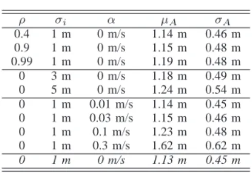
C. Peers self-positioning impact
In this section we measure the impact of the self-positioning model characterizing peers. To this end, we consider three different parameters: first, the correlation coefficient ρ among
successive self-positioning estimations of each peer; second, the self-positioning accuracy class σ of peers; third, the
accuracy driftα of peers. The other parameters are set to the
values of the reference case.
Table III gathers all the results. As it can be observed, the parameters have negligible impact on the accuracy of the opportunistic localization scheme that, hence, proves to be rather robust to localization errors of Peers. This is likely due to the fact that, despite the errors, the positions provided by the Peers form a uniform “cloud” of points around the User. Then, applying the barycentric scheme, the User always localizes itself near the center of such a cloud. To verify this conjecture, however, we plan to consider in future work other error models
TABLE III CORRELATION IMPACT ρ σi α µA σA 0.4 1 m 0 m/s 1.14 m 0.46 m 0.9 1 m 0 m/s 1.15 m 0.48 m 0.99 1 m 0 m/s 1.19 m 0.48 m 0 3 m 0 m/s 1.18 m 0.49 m 0 5 m 0 m/s 1.24 m 0.54 m 0 1 m 0.01 m/s 1.14 m 0.45 m 0 1 m 0.03 m/s 1.15 m 0.46 m 0 1 m 0.1 m/s 1.23 m 0.48 m 0 1 m 0.3 m/s 1.62 m 0.62 m 0 1 m 0 m/s 1.13 m 0.45 m
for peers estimation, such as model for podometers, or for MEMS-based inertial navigation systems, or for RSS-based landmarks.
D. Other parameters
In previous papers [8], [9], we also studied the impact of other parameters; we showed that the accuracy of the user self-positioning scheme degrades when: the amount of peers within range (N ) decreases, the range threshold R increases or
the peers mean speed µspeed decreases. We re-evaluate these
parameters and others quickly here.
For the setup used here, using 50 peers give a mean accuracy of 1.76 m while 200 peers give a mean accuracy of 0.77 m (this is not as overcrowded as it may seem, if you think of a station, a big mall or a conference room for instance: in a 100m×100m
square, this gives 50 m2 per peer). Of course, the more peers there are with random trajectories, the more communication opportunities there are, and the more information are fed to the LMI system, which induces better estimations.
Another way to improve the accuracy is to increase the waiting time of the user: 5 minutes lead to an accuracy of 0.91 m. In that case, the barycentric estimation takes into account more and more raw LMI estimations, thus giving less weight to bad raw estimations. On the contrary, reducing to 1 minute degrades the accuracy to 1.67 m.
We also changed the radio coverage range. A 5 m range leads to an accuracy of 1.01 m, while a 20 m range leads to an accuracy of 1.86 m. This is not an intuitive result, since a larger range would mean more opportunities for sharing information. However, these additional positions are more far away from the user, which increase both the raw LMI error and the barycentric error.
Finally, we also changed the mean peer speed. If peers are slow (0.6 m/s) the accuracy degrades to 2.14 m. If peers are fast (3 m/s) the accuracy improves to 0.68 m. When the speed increases, positions taken into account will largely vary between two successive LMI-only estimations. This diversication of spatial information improves the behavior of the barycentric estimation.
IV. RELATEDWORK
Self-localization problem has been investigated in a number of papers. Most common localization methods consist in
measuring the power of the received RF signal (RSSI), the Time of Arrival (ToA) or the Angle of Arrival (AoA) of the RF signals from the beacons. In this way, every node estimates a set of distances from the beacons and, then, guesses its position by means of lateration and triangulation techniques [10], [11] or by using statistical estimation methods [12]. Overviews of localization techniques based on RSSI and ToA measurements can be found in [13], [14], [15]. Multi-step localization techniques, which involve a number of successive refinement phases, have been proposed by Savarese [16] and Savvides [11]. Other solutions leveraging on specialized and complex hardware and infrastructure are given in [3], [2], [4]. When nodes (either static or mobile) can detect each other, then it is possible to devise cooperative position estimate techniques, which are very well studied in robotics. In [17] the authors utilize Markov localization for self-localize nodes and, then, probabilistic methods to synchronize robots estimate when they have a contact. Collective localization based on a distributed Kalman Filter is proposed in [18], whereas an anchor-free approach where robots infer their position estimate on the basis of the only information exchanged among them is proposed in [19].
In [7] Doherty et al. pioneered the use of semidefinite programming (SDP) methods in the localization problem. The problem is considered as a bounding problem containing several convex geometric constraints mathematically repre-sentated as linear matrix inequalities (LMI). The mechanism proposed in this paper is based on this approach, taking into estimation errors and introducing a barycentric improvement over time.
The Centroid localization method [20] is developed to estimate the user’s location by computing the barycenter of all the positions received from those fixed beacon nodes. To find the optimum deployment of those beacon nodes for a given application may consume a lot of labor.
In the APIT method [21], a user chooses three beacon nodes around him as the triangle vertex point and uses the APIT algorithm to test if he is lying in the triangle. If the APIT test can be passed, i.e., at least one node’s signal is becoming barycenter of the triangle will be taken as the location estimation of the user. Continuously, another different three nodes will be chosen to face the APIT test again. If the new test can also be passed, the barycenter of the intersection of the triangles will be used. By analogy, the user will repeat this APIT test until all combinations are exhausted or the satisfying accuracy is achieved. It is noticeable that since the APIT test is used under the condition of static beacon nodes, accomplishing it is still not an easy thing. Additionally, the APIT test may fail in less than 14% of the cases [21].
Other research works jointly solve the time synchronization and localization problems. For instance, Enlightness [22] relies on the availability of beacon nodes (at least 5% of the nodes) providing absolute time and space information, like the GPS in outdoor environments. Enlightness combines recursive positioning estimation [23] with a clock offset estimation scheme based on the measure of beacon packet delays and
timestamps.
In [24], an advanced integration of 802.11b equipments and Inertial Navigation System (INS) is used to enhance the perfor-mance of the indoor positioning system. As a result, a system performance close to the meter accuracy can be achieved with a low density of access points in the environment, provided that users carry inexpensive INS equipment.
V. CONCLUSION ANDFUTUREWORK
In this paper, we propose an algorithm in which a still user infers localization information using the positions of other passing-by nodes. The opportunistic interaction is modeled by considering several parameters that permit to compare the performance of the scheme in different scenarios.
In all the cases considered in this study, we obtained a localization error lower than 2.5 meters that can be reduced
to less than 1 meter with an accurate tuning of the system parameters. In particular, the duty cycle of the opportunistic-scan phase has been observed to have a significant impact on the user self-positioning estimation: the shorter the duty cycle the less the rendezvous probability with peers and, in turn, the lower the localization accuracy. Furthermore, we observed that the proposed opportunistic localization scheme is rather robust to the self-positioning error model for Peers. In fact, the correlation, the standard deviation and the drift of the self-positioning error do not significantly affect the localization accuracy, provided that the algorithm is performed over the data gathered with a large enough number of opportunistic exchanges.
In order to complete this work, some improvements will be done. We will try to define a more realistic set-up involving different types of peer nodes, e.g. access points with well-known positions but only partial coverage and mobile peers carrying cheap INS systems which accuracy drifts over time. We will also implement the opportunistic meeting model defined in [25] that applies to peer meetings. It is also possible to take into account different self-localization models and opportunistic update.
REFERENCES
[1] G. Zanca, F. Zorzi, A. Zanella, and M. Zorzi, “Experimental comparison of RSSI-based localization algorithms for indoor wireless sensor net-works,” in Proc. of the REALWSN’08 Workshop on Real-World Wireless
Sensor Networks, Glasgow, Scotland, April 2008, pp. 1–5.
[2] R. Want, A. Hopper, V. Falcão, and J. Gibbons, “The active badge location system,” ACM Transactions on Information Systems, vol. 10, no. 1, pp. 91–102, January 1992.
[3] H. S. Cobb, “Gps pseudolites: theory, design, and applications,” PhD Thesis, Stanford University, September 1997.
[4] Ekahau. [Online]. Available: http://www.ekahau.com
[5] “IEEE Std 802.15.1 - 2005 IEEE Standard for Information technology Telecommunications and information exchange between systems -Local and metropolitan area networks - Specific requirements. - Part 15.1: Wireless medium access control (MAC) and physical layer (PHY) specifications for wireless personal area networks (WPANs),” IEEE Std
802.15.1-2005 (Revision of IEEE Std 802.15.1-2002), 2005.
[6] “IEEE Standard for Information technology-Telecommunications and information exchange between systems-Local and metropolitan area networks-Specific requirements - Part 11: Wireless LAN Medium Ac-cess Control (MAC) and Physical Layer (PHY) Specifications,” IEEE
Std 802.11-2007 (Revision of IEEE Std 802.11-1999), 12 2007.
[7] L. Doherty, L. E. Ghaoui, and K. S. J. Pister, “Convex position estimation in wireless sensor networks,” in Proc. of IEEE INFOCOM, Anchorage, AK, USA, April 2001, pp. 1655–1663.
[8] G. Kang, T. Pérennou, and M. Diaz, “Barycentric location estimation for indoors localization in opportunistic wireless networks,” in Proc. of the
Second International Conference on Future Generation Communication and Networking (FGCN 2008), Sanya, China, December 2008, pp. 220–
225.
[9] ——, “An opportunistic indoors positioning scheme based on estimated positions,” in Proc. of the IEEE Symposium on Computers and
Commu-nications (ISCC’09), Sousse, Tunisia, July 2009.
[10] A. Savvides, H. Park, and M. B. Srivastava, “The n-hop multilateration primitive for node localization problems,” Mobile Network Applicatons, vol. 8, no. 4, pp. 443–451, August 2003.
[11] ——, “The bits and flops of the n-hop multilateration primitive for node localization problems,” in Proc. of the 1st ACM international workshop
on Wireless sensor networks and applications (WSNA’02), Atlanta, GA,
USA, September 2002, pp. 112–121.
[12] N. Patwari, R. O’Dea, and Y. Wang, “Relative location in wireless net-works,” in Proc. of the IEEE VTS 53rd Vehicular Technology Conference
(VTC 2001 Spring), Rhodes, Greece, May 2001, pp. 1149–1153.
[13] N. Patwari, J. N. Ash, S. Kyperountas, A. O. Hero III, R. L. Moses, and N. S. Correal, “Locating the nodes: cooperative localization in wireless sensor networks,” IEEE Signal Processing Magazine, vol. 22, no. 4, pp. 54–69, July 2005.
[14] A. Savvides, M. Srivastava, L. Girod, and D. Estrin, Localization in
sensor networks. Norwell, MA, USA: Kluwer Academic Publishers, 2004, pp. 327–349.
[15] R. Huang and G. V. Zaruba, “Static path planning for mobile beacons to localize sensor networks,” in Proc. of the 5th Annual IEEE International
Conference on Pervasive Computing and Communications Workshops (PerCom Workshops 2007), White Plains, NY, USA, March 2007, pp.
323–330.
[16] C. Savarese, J. M. Rabaey, and K. Langendoen, “Robust positioning algorithms for distributed ad-hoc wireless sensor networks,” in Proc. of
the 2002 USENIX Annual Technical Conference, San Francisco, CA,
USA, August 2002, pp. 317–327.
[17] D. Fox, W. Burgard, H. Kruppa, and S. Thrun, “A probabilistic approach to collaborative multi-robot localization,” Autonomous Robots, vol. 8, no. 3, pp. 325–344, June 2000.
[18] S. Roumeliotis and G. Bekey, “Collective localization: a distributed kalman filter approach to localization of groups of mobile robots,” in Proc. of the 2000 IEEE International Conference on Robotics and
Automation (ICRA ’00), vol. 3, San Francisco, CA, USA, April 2000,
pp. 2958–2965.
[19] A. Howard, M. Matari´c, and G. Sukhatme, “Localization for mobile robot teams using maximum likelihood estimation,” in Proc. of the
IEEE/RSJ International Conference on Intelligent Robots and System (IROS 2002), Lausanne, Switzerland, October 2002, pp. 434–439.
[20] N. Bulusu, J. Heidemann, and D. Estrin, “Gps-less low cost outdoor localization for very small devices,” IEEE Personal Communications
Magazine, vol. 7, no. 5, pp. 28–34, October 2000.
[21] T. He, C. Huang, B. M. Blum, J. A. Stankovic, and T. Abdelzaher, “Range-free localization schemes for large scale sensor networks,” in
Proc. of the 9th Annual International Conference on Mobile computing and networking (MobiCom ’03), San Diego, CA, USA, September 2003,
pp. 81–95.
[22] A. Boukerche, H. A. B. F. de Oliveira, E. F. Nakamura, and A. A. F. Loureiro, “Enlightness: An enhanced and lightweight algorithm for time-space localization in wireless sensor networks,” in Proc. of the 13th
IEEE Symposium on Computers and Communications (ISCC 2008),
Marrakech, Morocco, July 2008, pp. 1183–1189.
[23] J. Albowicz, A. Chen, and L. Zhang, “Recursive position estimation in sensor networks,” in Proc. of the 9th International Conference on
Network Protocols (ICNP 2001), Riverside, CA, USA, November 2001,
pp. 35–41.
[24] F. Evennou and F. Marx, “Advanced integration of wifi and inertial navigation systems for indoor mobile positioning,” EURASIP Journal
on Applied Signal Processing, pp. 1–11, 2006.
[25] F. Zorzi and A. Zanella, “Opportunistic localization: modeling and analysis,” in Proc. of the IEEE 69th Vehicular Technology Conference