Life Gallery: event detection in a personal media collection.

(1)

HAL Id: hal-01327887

https://hal.archives-ouvertes.fr/hal-01327887

Submitted on 7 Jun 2016

HAL is a multi-disciplinary open access

archive for the deposit and dissemination of

sci-entific research documents, whether they are

pub-lished or not. The documents may come from

teaching and research institutions in France or

abroad, or from public or private research centers.

L’archive ouverte pluridisciplinaire HAL, est

destinée au dépôt et à la diffusion de documents

scientifiques de niveau recherche, publiés ou non,

émanant des établissements d’enseignement et de

recherche français ou étrangers, des laboratoires

publics ou privés.

Life Gallery: event detection in a personal media

collection.

Antoine Pigeau

To cite this version:

Antoine Pigeau. Life Gallery: event detection in a personal media collection.: An application, a basic

algorithm and a benchmark. Multimedia Tools and Applications, Springer Verlag, 2017, Multimedia

Tools and Applications, �10.1007/s11042-016-3576-y�. �hal-01327887�

(2)

Life Gallery: event detection in

a personal media collection

An application, a basic algorithm and a benchmark

Draft version

Antoine Pigeau

DUKe research group

LINA (CNRS UMR 6241)

2, rue de la Houssini`

ere 44322 Nantes cedex 03 - France

antoine.pigeau@univ-nantes.fr

June 7, 2016

Abstract

Usage of camera-equipped mobile devices raises the need for automatically organizing large personal media collections. Event detection algorithms have been proposed in the literature to tackle this problem but a shortcoming of these studies resides in the lack of comparison of the different solutions. The goal of this work is then to provide a set of tools for the assessment of an event detection method.

Our first contribution is our prototype Life Gallery, which aims to retrieve metadata of a personal media collection in order to facilitate the building of a benchmark. Our second con-tribution is an event detection algorithm based on successive refinements of an initial temporal partition. Our solution uses a simple algorithm that regroups consecutive similar media or split groups with dissimilar media.

The choice to provide a basic solution is to compare in a future work our results with more complex solutions, in order to really assess the benefit of these latter. Finally, our third contribution is a benchmark of 6 different users’ collections obtained thanks to our Life Gallery application.

1 Introduction

Large personal media collections are now widespread thanks to the availability of cheap smart phones equipped with a camera and high capacity memory card. Users have now an access to their entire life directly through their mobile device, leading to the need for efficient methods to retrieve/browse their media (image, video and why not text file). This latter requirement is in addition stressed by the recent availability of cloud services that leads to higher capacity storage and even multiple data

(3)

source. Browsing or searching for a specific subset of media in large personal collection on a mobile device still remains an open issue.

While experiments [1] show that the time dimension is the favourite criterion for the browsing task, a remaining problem lies in the large time window of the collection. Indeed, a collection usually regroups events of a user’s life that can spread over several years. Retrieving a specific event is thus tricky with the basic GUI provided on the mobile device: usually a temporally ordered matrix of thumbnails. The only way here to find a specific media is to accurately remember its date, which is usually an information that we lost as time goes by. Improving time line with adapted interface must be provided to ease the browsing task on a mobile device.

Event detection was proposed to deal with such an issue, available for example on Apple iPhoto or the Android Gallery application. An event is defined as a set of media taken on a same occasion, for instance, a party, a birthday or a one-week vacation. The building of such events is based on the media content (image pixels) and the availability of several metadata, as EXIF metadata, including the timestamps, the locations, the user tags, the technical properties (aperture, exposure time, . . . ). A clustering process can then be applied on those metadata to retrieve the event: practically, it consists to detect the meaningful gap between temporally consecutive media (for example, a temporal, a location, or a user tag change).

1.1 Objective

While several methods have been proposed to tackle the event detection in a personal media col-lection, few works really compare their results with each other. Our purpose is then to provide the necessary tools for such a comparison:

• an application to easily retrieve metadata from a user collection and to create manually an event partition;

• a basic event detection solution in order to study in a future work the real gain of more complex clustering algorithms. Note that no comparison with another methods is carried out in this paper;

• a benchmark of users’ collections, in order to test various methods on a same test data set.

1.2 Contributions

Our first contribution is our prototype Life Gallery, an android application available for free on the Google Play store. The objective of this prototype is threefold:

• to provide all the tools to update/export all the metadata of a user collection;

• to provide a specific interface to the user in order to create a truth partition. This truth partition is then used to assess our clustering algorithms;

(4)

Our second contribution is a basic event detection algorithm based on the following metadata included in each media: the timestamp, the geographical coordinate, the user tag and the media content, based on the Scale-Invariant Feature Transform [2] (SIFT). Our proposal works as follow: successive filters are applied on an initial temporal partition in order to detect the meaningful gap between events of a personal collection. A filter is merely a simple algorithm that specifically works with one metadata. It takes as input an event partition, applies either merge or split operations on events, and outputs a new event partition. A filter is exclusively a split filter or a merge filter. For instance, a temporal merge filter followed by a geographical merge filter can be applied on an initial temporally ordered collection (a list of temporally ordered groups, where each group contains just one media). Such a partition consists then to first regroup media documents that are temporally close in an event and then to merge together successive events that are geographically nearby.

The tricky point resides here in determining the best combination of filters to provide the event partition. Indeed, in our context, 4 different metadata are used with two different modes, a merge filter or a split filter, leading to around 55000 filter combinations. All those possible combinations are tested in our experiment section on several personal media collections.

One gain of such an experiment is also to study the relevance of the previous metadata for the event detection. To our knowledge, no work investigate yet the different ways to combine the available metadata to cluster a personal media collection. Relevant questions as which dimension to use ? which are not worth using ? in which order to apply them ? still remain an open issue.

Finally, our last contribution is a benchmark composed of 6 users’ collections. For each collection, the following data are provided:

• a truth partition carried out manually by the user himself thanks to our Life Gallery applica-tion;

• the metadata obtained from the collection. For each media, its timestamp, its location, its user tags and a set of SIFT keypoints are provided.

This benchmark is available on the Life gallery website [3] and will be used in a future work to compare the results obtained with our basic approach and other methods proposed in the literature. The remainder of this paper is organized as follow: section 2 surveys works related to personal collection management. Section 3 presents our prototype Life Gallery and is followed by the pre-sentation of our clustering process in section 4. Experiments are proposed in section 5. Finally, the work is summarized and perspectives are sketched in section 6.

2 Related Work

Timestamp uses to be a favourite criterion to index a personal image collection. Its availability leads to several works [4, 5, 6, 7] on the incremental segmentation of a time-stamp sequence. Detection of meaningful gaps enables to find events or hierarchy of events [6] in the collection. Such a boundary could be arbitrary defined or obtained from the average gap over a temporal window. A most recent work [7] uses time series to model the time distribution of the personal image collection. Based on

(5)

a one year calendar, a method is proposed to compute a model automatically. As in our previous work [8] where timestamps are modelled with a Gaussian distribution, such methods face with the issue to obtain a correct model with complex parameters.

Works on personal image indexation also deal with the image localization [9, 10, 11, 12]. Indeed such a meta-data is easily available thanks to GPS system directly integrated in each smart phone, and helpful to automatically annotate the image [10, 13]. Several software solutions, as for example the WWMX system [9] or Flickr, propose a map-based interface to browse the collection. The main problem of such an approach is that the map gets cluttered with a huge number of images. Several solutions were proposed to summarize an image set: the work [9] proposes to aggregate images in accordance with the map scale, while [12] selects representative images from multi user collection based on their meta-data. Note that our event detection algorithm could also be relevant to ease the browsing task of media on a map: an event represents a set of media taken on one or several specific locations. Browsing events on a map, instead of specific media, could present interesting advantages.

Combinations of the two previous criteria are of course proposed in numerous works [8, 14, 11, 15, 16]. Naaman et al.[14] propose to hierarchically organize an image collection, while [11] provides a one level partition. To our understanding, [14] incorporates a series of rules derived from user’s expectations to build a geo-temporal hierarchy of events. Based on an ensemble clustering method, [16] proposes to combine two temporal and geographical partitions by selecting the best temporal or geographical clusters. Because an exhaustive search for all the possible combinations is not feasible, a heuristic is provided to build the merge. Unfortunately, the cost of the merge could be problematic on a mobile device, where the collection is often updated.

Few works [17, 18] propose solutions based on contextual metadata while they are of much interest for the search or browsing task. Experiments in [19] depict the user’s favourite criteria: it resorts that the first ones are the indoor/outdoor property, the people, the location and the event. While accurate indoor/outdoor detection methods exist [20] and that reverse geo-tools can provide rich location information obtained from the GPS coordinate, the presence of both event and people tags remains still a challenge since media are usually poorly annotated [1, 21]. Nevertheless the tag availability could increase due to strong effort to help users in this task, as face detection algorithm or collaborative tagging [21, 22].

The importance of user annotation is showed in the following works. CAMELIS [17] uses rich metadata to browse a personal image collection. Each image contains metadata on several attributes which values are partially ordered (subsumption relation - Paris is included in France for example). Browsing task is then carried out by selecting keywords in the hierarchy values of each attribute. Das et al. [18] emphasize recurring themes of a user’s collection. Their proposal consists to extract metadata of each media based on high and low features, such as EXIF header, the image content or the face detection. Frequent itemsets, defined as groups that share several metadata in commons, are then automatically retrieved. Contrary to these previous works, our proposal uses text annotation only to improve an existing partition. The user is then pushed to annotate his/her event in order to update the actual groups detected. For instance, tagging of two consecutive groups with similar

(6)

Figure 1: From the left to the right: the event view, the map view and the album view of Life Gallery application. On the event view, each line represents an event. The displayed images on each line are a summary of their associated events. Here the summary size is defined with 3 images. keywords would result to merge them in a same event.

To our knowledge, all these previous works on event detection rarely compare their proposals with one another on a common test data set. This latter point is the purpose of our application Life Gallery.

3 Life Gallery

The application Life Gallery is available on the market Google Play since 2010 and has now around 2000 active users. This application is implemented by the DUKe team with the contribution of the students of the University of Nantes.

Roughly, this application is a Gallery software that contains all the common functionalities to browse a user collection. The benefit of Life Gallery is the inclusion of clustering algorithms, tag tools and specific GUI, that aim to ease the organization and the browsing task of the user’s media. Thanks to the availability of the application on the Google Play market, this prototype will provide us an access to a large set of users. Each user has the possibility to share with us all his collection’s metadata and an associated truth partition, carried out manually by the user himself.

In the following, we present the user interface, the tag tools and the interface to build a truth partition.

3.1 Graphical User Interface

(7)

Figure 2: From the left to the right: the text tag view, the location tag view and the favourite locations saved. The new location is set from a favourite location or by browsing the map and touching the map on the new location.

• event view: all the events are displayed in a list ordered temporally from now to the past. The list of events is obtained thanks to an event detection algorithm;

• map view: the media locations are displayed on a map. Users can then browse the media associated to each pin;

• album view: albums are created automatically from the user’s textual annotation. Each text tag involves the creation of its associated album;

• directory view: all the directories that contain at least one media document are displayed. Figure 1 shows the different views to browse the user collection. On the event view, each element represents an event: an event is represented by a summary composed of a subset of the media included. Only the first media document, the second and the last one of the group are presented. Nevertheless, the choice of the media to display remains an open issue. A selection based on the image quality, its content or its representativeness in accordance with the event would be pertinent. A click on an event opens a gallery view that displays all the media contained in the selected event. The map view, album view and directory view are not detailed here since they are relatively common.

3.2 Media Tag

Tagging the media is a useful information to take into account to organize automatically the user collection. We then propose two tools, respectively for the text tag and the location tag. For both, the users first selects a set of events or a set of media and then tag them:

(8)

• for the text tag, the user just types the keywords and adds them to the group or to a specific media document;

• for the location tag, the user can select a new location on the map to apply directly on a media group. To ease the task, users have the possibility to save their favourite locations. Geotagging of events located in common places is then quickly done.

The figure 2 presents the interface for the keyword and geographical tag.

3.3 Building of a test data set

In order to assess event detection algorithms, we need the following data for each collection: the metadata of each media document and an event partition carried out manually by the user. Life Gallery proposes then a tool to export all the media metadata to xml format (for all media, the timestamp, the location, the keyword and the SIFT keypoints) and a dedicated interface to create a manual partition to obtain the true events of the collection. The figure 3 shows the interface to build this truth partition, where a user can merge or divide an initial event partition.

Each partition generated by an event detection algorithm will be compared to the truth partition to assess its quality.

4 Event detection algorithm

The second contribution of this work is to provide a basic event detection algorithm of a personal media collection, based on the different available metadata: the timestamps, the locations, the tag annotations and the SIFT keypoints.

Our proposal is a successive refinement of an initial temporal partition. This initial partition I0

is set to a list of all the media temporally organized: each group of this partition is composed of one media document. The final partition is obtained by applying several refinements, each one leading to a temporal partition.

This choice to constraint the user with a temporal view is motivated by the way a user browses his/her collection on a mobile device:

• experiments on users [1] show that the temporal dimension is the favourite criterion to browse the collection. The main advantage of this dimension is that the users, based on his memory, know the structure of their collections and can determine the position of one event among the others;

• graphical user interface presents constraints on mobile. Existing mobile interfaces to browse media propose a list view to scroll the collection (or a matrix of media), generally associated to a time line. Keeping the same solution to display a list of events seems then convenient. In the following, we first define a media document and a group of media. Next, we present our refinement algorithm based on a set of filters. These filters are then explained in details.

(9)

Figure 3: Building a truth partition: the top row shows a merge example while the bottom one shows a division. On the top row, the first figure depicts the initial events, the second the selected events to merge (both events of the first row and both events of the third row) and the last figure, the result obtained after the merge. Only consecutive events selected by the user are merged. On the bottom row, the first figure shows the initial event and the selected event to divide (second event on the first row), the second figure presents the division to process in the selected event (a division is done for each change selected/unselected - here the event is divided in 3 groups: the first 4 media selected, then 3 not selected media, and the three last ones selected) and the last figure displays the result of the division. The selected event is now divided in three groups (second event of the first row with 4 media, and both events of the second row with 3 media each).

4.1 Media and group definition

Let a personal multimedia collection be composed of N media. We define here a media document as an image or a video document. Each media Mi, i ∈ [1, N ], is defined with the following properties:

Mi= {ti, (lati, longi), {wi1, . . . , wiL}, {SIF Ti1, . . . , SIF TiS}} (1)

where tiis the timestamp (unity is millisecond), (lati, longi) the geolocalization defined with the

(10)

the set of S SIFT keypoints included in the media document.

For example, two images 1 and 2 taken respectively on 2012/04/05 04:14AM in Paris, annotated with the keywords [Paris, Parc], and on 2012/04/05, 04:15AM in Paris, annotated with the keywords [Paris, Street ], are defined as:

M1= {1 333 576 800 000, (48.889146, 2.246340), {P aris, P arc}; {SIF T }}

M2= {1 333 576 860 000, (48.889144, 2.246330), {P aris, Street}{SIF T }}

A group containing n media is then defined with the following properties:

Gj= {nj, tj, (latj, longj), {(α1, wj1), . . . , (αL, wjL)}, SIF Tj, {M1, . . . , Mn}} (2)

where nj is the number of media in the group, tj the timestamp of the group, gjits geolocalization,

{(α1, wj1), . . . , (αL, wjL)} a list of keywords where each keyword wjl is associated with a weight

αl, SIF Tj the union of SIFT keypoints of the media and {M1, . . . , Mn} the media included in the

group. The weight αlassociated to a keyword wjl represents the number of times it appears in the

group.

A group G1containing M1and M2is then defined as follows:

G1= {2, 1333576830000, (48.889145, 2.246335),

{(2, P aris), (1, P arc), (1, Street)}, {M1, M2}}

Timestamp and location of G1are set to the average values of the group. Our solution to compute

the timestamp and the location of a group is discussed in section 4.3.1.

4.2 Refinement of the initial partitions

In order to build our event partition, we propose to apply successively several filters on the collection. Each filter can be set with two modes, merge or division. A filter refines then a partition just by merging or dividing groups. Here are the description of the different sort of filters to apply: 1. the temporal filter refines a partition thanks to the timestamps: temporally close media are

merged while a big gap involves two separate events;

2. the geographical filter refines a partition based on the geographical coordinates: a set of temporally successive groups are merged if they belong to a same location while a group with several locations is divided;

3. the keyword filter refines a partition based on the user textual annotations. For example, a set of successive groups are merged if they contain similar keywords while a group with different keywords is divided. An interest of this filter is to provide a way for users to interact with the clustering process, i.e, to correct a partition just by tagging their groups;

(11)

Require: N media

Require: a set of filters {F1, . . . , FK}

1.Creation of the initial partition I0:

for each media mi do

create a new group gj

add mi in gj

end for let P = I0

2.Apply the filters: for each filter Fk do

P = Fk(P )

end for

return the refined partition P

Algorithm 1: Main algorithm: creation of the initial partition followed by the application of a set of filters on the user collection.

4. the SIFT filter refines a partition based on the features of the media. The SIFT algorithm [2] is used to retrieve those features. As for the previous filters, the approach consists to merge or divide media groups with respectively similar and different image contents.

For example, an interesting way to partition a user collection could be to apply a merge temporal filter followed by a division geographical filter. Practically, it would regroup close temporal events and then divide these groups if they contain several locations.

One issue of such a solution based on filters is now to choose their best combination among the thousands of possibilities. Indeed, all the filters are independent and can be applied in any order.

The main procedure applied on the user collection is detailed in the algorithm 1. In the following, the filters and their specificities are detailed.

4.3 Definition of a filter

As explained above, our proposal is to apply successively a list of filters to refine an initial partition. Each filter is defined with the following attributes:

• a type, temporal T , geographical G, keyword K or SIFT S; • a mode, defined with merge M or division D;

• a similarity function similarity(), used to compute the similarity between two groups (merge) or between two media documents (division);

• a threshold: use to determine if a merge or a division is applied.

For example, we can define a merge temporal filter TM =< similarity(), 3600ms > that regroups

two consecutive events if their temporal distance is lower than 1 hour. Here the function similarity() computes the temporal gap between two consecutive groups and 3600ms is the threshold.

(12)

Require: a partition P to refine, composed of a set of groups {G1, . . . , GJ}

Require: a filter typeM < similarity(), threshold >

while j = 1 < sizeOf P artition(P ) do sim = similarity(Gj−1, Gj)

if sim < threshold then add all media of Gj in Gj−1

remove the group Gj

else j = j + 1 end if end while

Algorithm 2: Merge Filter: consecutive groups are parsed in a temporal order. Two consecutive groups are merged if their similarity is lower than the specified threshold.

For practical reasons, each combination of filters is named with only the attributes used and its mode. The previous example, a merge temporal filter followed by a division geographical filter, is then represented with GD(TM(I0)), where I0 is the initial partition (one media document per

group).

The process of a filter depends on its type:

• merge filter: the process consists to parse all the groups of a partition, computing the similarity between each consecutive groups. If the similarity is lower than the threshold of the filter the groups are merged;

• division filter: the process consists to parse the content of each group. If two consecutive media documents have a higher similarity than the threshold of the filter, the group is divided. The algorithms 2 and 3 detail respectively the merge and division processes to refine a partition.

Two problems remain to compute our similarity:

• how to deal with the similarity between two groups or two media documents on each meta-data ? while the spatial or temporal similarities are simple (average, median, minimum or maximum,. . . ), the keyword and SIFT matching similarities are more complex;

• how to deal with the missing values ? each metadata element presents different levels of availability, from the timestamp that is supposed to be always present to the user tag that is rarely set.

In the following, we first depict our similarity functions and then present our solution to manage the missing values.

(13)

Require: a partition P to refine, composed of a set of groups {G1, . . . , GJ}

Require: a filter typeD< similarity(), threshold >

while j = 0 < sizeOf P artition(P ) do size = sizeOf Group(Gj)

for i = 1 to size do

sim = similarity(Mi−1, Mi)

if sim > threshold then

create a group Gnew containing the media Ml for l in [i, size]

add the group Gnew at position j + 1

break{pass to the new group} end if

end for j = j+1 end while

Algorithm 3: Divide Filter: for each group, the media are temporally parsed. If two consecutive media documents have a similarity higher than the specified threshold, the group is divided.

4.3.1 The temporal and geographical similarity

A convenient temporal or spatial similarity function between two consecutive media documents is the Euclidean distance. The issue here is thus not the similarity function to use but the way to represent the timestamp or the location of a media group. Several functions could be used as the average, the median or the min and max functions.

In our context, the median solution would be rather similar to the average since our groups have a limited size and a small range. A solution based on the minimum and maximum function was also considered. For the temporal similarity, it consists to compute the distance with max(Gi)−min(Gj)

for two consecutive groups (with i prior to j). Adapted to the geographical similarity, this latter solution consists to compute the distance based on the two closest media of the two groups. But this latter solution does not take into account the distribution of the media in the group.

To conclude, our solution is to use the average function. A group of media is thus represented by the average of its timestamps and the average of its locations.

4.3.2 The Keyword similarity

Our goal is to merge or divide consecutive groups of media with keyword similarities. Remind that each group is represented as a bag of words. The weight associated to each keyword is the number of time it appears in the group. A group of media is then considered as a short text document.

A variety of measures exists to compute a similarity between text documents [23]. Most popular criteria are the Euclidean distance, the cosine similarity, the Jaccard correlation coefficient, the Dice coefficient or the Kullback Liebler divergence. All these criteria were compared in [23, 24] and the conclusion is that the Euclidean distance is the worst while the others present similar performance.

(14)

Note that in our context, each document contains either few or no keywords, so that the use of common improvement used in the area of document clustering as term frequency - inverse document frequency (tf-idf) or stop word detection is not relevant.

We then opt here for a slight adaptation of the cosine similarity, due to its independence face to the document keyword proportion:

SimilarityK(Gj, Gj0) = 1 − PL l=1 tjl× tjl nj ×tj0l× tj0l nj0 q PL l=1(tjl)2× q PL l=1(tj0l)2 (3)

Where tjl= tf (Gj, wl) is the frequency of the term wlin the group Gj, L = nj+ nj0 is the number

of different terms in the union of Gj and Gj0 (n_j is the size of the group G_j). For a media, the

function tf () returns always 1 while for a group, it returns the weight α associated to each keyword (see definition 2). The adaptation of the cosine similarity concerns here the term tjl×tjl

nj that weights

the frequency of the keyword in accordance with its number of apparition in the group. Practically, it decreases the weigh of a keyword that appears only in few media documents of the group.

For example, let two groups G2and G3 be defined as:

G2= {2, 1333576833600, (48.889145, 2.246335),

{(2, Arthur)}} G3= {6, 1333576833789, (48.889145, 2.246335),

{(1, Arthur)}}

G3is composed of 6 media, with one document associated to the keyword Arthur. To our opinion,

a low similarity between the two groups would be pertinent (we do not want to merge those two groups just because G3 contains the same keyword in only one of its media document). But with

the classic cosine measure, the score obtained would be 0, leading to a full similarity. With our adaptation, the similarity is significantly lower:

t21= tf (G2, Arthur) = 2 t31= tf (G3, Arthur) = 1 SimilarityK(G2, G3) = 1 − 2×2 2 × 1×1 6 √ 22_×√₁2 SimilarityK(G2, G3) = 1 − 1 6 = 5 6

Our adaptation of cosine similarity is non negative and bounded in [0, 1]. The score 1 is obtained if the two events do not present similar keywords while 0 is reached if the two events contain the same keywords with proportional weight with respect to their size.

4.3.3 The SIFT similarity

The SIFT algorithm [2] aims to retrieve local scale invariant features in an image. Each feature is invariant to geometric transformation and described with a vector descriptor. SIFT matching

(15)

between pictures is then carried out thanks to a similarity between SIFT keypoints, usually the Euclidean distance. Keypoints match if their distance is lower than a certain threshold. Two pictures are similar if they present matching keypoints.

In our context, our requirement is a similarity between two events, where each event is defined with a set of keypoints obtained from the union of included media’s keypoints. Note that for each set obtained from an event, we remove keypoints that match together. In some way, we remove the duplicate keypoints of one event.

To compare two groups, we opt for the following similarity: SimilaritySIF T(Gj, Gj0) = 1 −

M atch(SIF Tj, SIF Tj0) + M atch(SIF T_j0, SIF T_j)

|SIF Tj| + |SIF Tj0|

(4) where SIF Tj is the set of keypoints of event j and M atch(Gj, Gj0) a function that returns the

keypoints of event j that match event j0. This score is symmetric and bounded in the interval [0, 1] (ambiguous matches, obtained if a keypoint matches with more than one point, are removed).

Note that the function M atch() is not symmetric. For instance, let two images j and j0 be defined with respectively 3 and 2 keypoints. All of the keypoints of j can match the ones of j0 leading to a matching score of M atch(SIF Tj, SIF Tj0) = 3 and all the keypoints of j0 can also

match the keypoints of j leading to a score of M atch(SIF Tj, SIF Tj0) = 2. The similarity obtained

on this example is then SimilaritySIF T(j, j0) = 1 −3+2₅ = 0.

4.3.4 Dealing with the missing values

While timestamps of media are usually present, location, keyword and SIFT keypoints are often not defined. The computation of the similarity between media with empty value is then not obvious since it can be interpreted differently in accordance with the mode of the filter. Let’s see an example for two consecutive media documents containing no value for the location or the keyword:

• for a merge filter, these media are merged if their similarity is small. If no values is available, a large similarity should then be returned, in order to avoid a merge;

• for a division filter, these media are separated if their similarity is large. If no values is available, a small similarity should then be returned, in order to avoid a division.

To conclude, two media documents with no metadata must be considered far apart for a merge filter, and nearby for a division filter. Our solution consists then to interpret an empty value differently for both filters:

• merge mode: if one or both operands have no value, a high score is returned, to avoid a merge action;

• division mode: if one or both operands have no value, a low score is returned, to avoid a division action.

(16)

User Size of From To % of % of the collection localized media tagged media user #1 2933 10/05/2010 12/26/2013 100 62.9 user #2 3482 12/26/2009 08/14/2014 77.42 78.3 user #3 637 08/24/2012 12/12/2014 84.30 0 user #4 678 10/17/2013 03/02/2015 14.15 6.5 user #5 490 07/13/2013 03/25/2015 68.77 70.6 user #6 4371 03/29/2013 11/06/2013 92.03 0

Table 1: Properties of the user collections use in the experiment.

5 Experiments

Our last contribution is a benchmark composed of 6 media collections. With the help of our Life Gallery application, each user provided all the metadata of their media collection and built a manual partition that represents the true events of their collection. The properties of each collection is depicted in the table 1. For each collection, the user name, the number of media, the begin and end dates, and the number of tagged media are displayed. Each collection was composed of images and videos. Note that the SIFT keypoints were retrieved only for the images and not for the videos.

Our experiments consist to apply all the combinations of filters on each collection. Our objective is to assess the quality of our basic algorithm, studying the importance of each metadata and emphasizing the combinations that provide the best event detection.

In the following, we first present the notation used to name our filter and the score associated to each partition obtained. The results of the experiments are then presented and few comments are done on the relevancy of each metadata. Finally, we present the best average combination of filters obtained on the user collections.

5.1 Filter combination

The experiment consists to test all the combinations of filters on the 6 user collections. We have 4 types of filter, one for each metadata, and each filter is defined with a mode, division or merge. So that it amounts to apply 54799 combinations on each collection (combinations starting with division filters, or just composed of division filters, are obviously removed).

As a reminder, each filter is named with the metadata used - T temporal , G geographical, K keyword, S SIFT - and the mode - M merge or D division. GD(TM(I0)) is then a temporal merge

filter applied on the initial partition, followed by a geographical division filter.

For each filter combination, the partition obtained is compared to the truth partition provided by the owner of the collection. A score is computed based on the precision and recall criteria:

• precision = |set of truth groups ∩ set of groups obtained | | set of groups obtained |

• recall = |set of truth groups ∩ set of groups obtained| |set of truth groups|

(17)

# Combination Filter # of Recall (%) Precision (%) F2 (%) groups - Simple combinations - - - -1 TM(I0) 596 65.38 45.30 60.05 2 GM(I0) 506 63.44 51.78 60.70 3 TM(GM(I0)) 424 61.02 59.43 60.69 4 GM(TM(I0)) 426 61.26 59.39 60.88

- Best minimum combinations - - - -5 KM(TD(GD(GM(TM(I0))))) 521 71.91 57.01 68.34 KM(GD(TD(GM(TM(I0))))) KM(TD(GM(GD(TM(I0))))) 6 KM(TD(GM(SM(I0)))) 523 71.67 56.60 68.05 7 KM(TD(GM(I0))) 521 71.43 56.62 67.88 8 KM(GM(I0)) 392 64.41 67.86 65.07

Table 2: Evaluation of several combinations of filters on the user #1’s collection. For each evaluation, the number of groups, the recall, the precision and the F2 criterion are presented.

# Combination Filter # of Recall (%) Precision (%) F2 (%)

groups - Simple combinations - - - -1 TM(I0) 558 46.31 16.85 34.31 2 GM(I0) 1652 31.53 3.87 12.99 3 TM(GM(I0)) 529 43.84 16.82 33.18 4 GM(TM(I0)) 509 46.80 18.66 35.96

- Best minimum combinations - - - -5 KM(KD(GM(TM(I0)))) 263 71.92 55.51 67.91

6 GM(TM(KM(I0))) 253 68.47 54.94 65.26

7 TM(KM(I0)) 269 67 50.56 62.90

8 KM(I0) 925 62.07 13.62 36.27

(18)

# Combination Filter # of Recall (%) Precision (%) F2(%) groups - Simple combinations - - - -1 TM(I0) 110 66.67 41.82 59.59 2 GM(I0) 298 49.28 11.41 29.62 3 TM(GM(I0)) 108 66.67 42.59 59.90 4 GM(TM(I0)) 105 68.12 44.76 61.68

- Best minimum combinations - - - -5 GM(TD(TM(KM(I0)))) 192 43.48 31.25 40.32

6 GM(TM(SM(I0))) 190 42.75 31.05 39.76

TM(GM(SM(I0)))

TM(SM(GM(I0)))

(19)

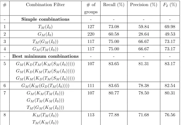
# Combination Filter # of Recall (%) Precision (%) F2 (%) groups - Simple combinations - - - -1 TM(I0) 127 73.08 59.84 69.98 2 GM(I0) 220 60.58 28.64 49.53 3 TM(GM(I0)) 117 75.00 66.67 73.17 4 GM(TM(I0)) 117 75.00 66.67 73.17

- Best minimum combinations - - - -5 GM(KD(TM(KM(SM(I0))))) 107 83.65 81.31 83.17 GM(KD(KM(TM(SM(I0))))) GM(KM(KD(TM(SM(I0))))) 6 GM(KM(GD(TM(I0)))) 111 83.65 78.38 82.54 7 GM(KM(TM(I0))) 107 80.77 78.50 80.31 GM(TM(KM(I0))) TM(GM(KM(I0))) 8 KM(TM(I0)) 113 77.88 71.68 76.56 TM(KM(I0))

- Best minimum combinations - - - -5 SM(TD(TM(GM(I0)))) 385 65.66 68.05 66.13

6 TD(TM(GM(I0))) 386 65.41 67.62 65.84

7 SM(TM(I0)) 392 64.16 65.31 64.39

(20)

• the results are then ordered with the F2 score, where

Fβ= (1 + β2) ×

precision × recall (β2_{× precision) + recall}

, which weights recall higher than precision. We favour a bit the recall because our main purpose is to retrieve the real events (a poor precision just indicates that some real events are unfortunately divided in several groups).

For these experiments, the parameters for all the temporal, the geographical, the keyword and the SIFT filters were respectively set to 3 hours, 30 meters, 0.4, 0.95 (few keypoint matchings are necessary to find a similarity between events).

The tables 2, 3, 4, 5, 6 and 7 present the scores obtained for the precision, recall and F2 for

each collection. On each table the first part depicts the score for simple combination based on the temporal and geographical metadata. The second part shows the best minimum combinations obtained with all the metadata. Note that several combinations can lead to identical score.

5.2 Few words on each collection

The collection user #1 is composed of almost 3000 media spanned over 2 years and 2 months. All the media have a location and 62.9% of them are tagged. The results in table 2 on lines 5 and 6 show that similar scores are obtained for filters based on the temporal and geographical metadata. For a single filter or a combination based on these metadata, the F2 score obtained is around 60%

(lines 1-4). Time and location seem then to be equally relevant for this collection, where 100% of the media are correctly tagged geographically. The best combinations are presented in the table 2 lines 5-8. The scores obtained are between 65% and 68%. For the best filter on line 5, the gain compared with a simple filter is of 8%. It is obtained with the use of the keyword filters and a geographical division filter.

The collection user #2 contains around 3500 media spanned over 4 years. 77.3% of the media are located and 78.3% are tagged. Results on the collection user #2 presented in table 3 are quite different from the user #1 since the filters based on geographical and temporal metadata present a low F2 score, around [12 − 30]%, as showed on lines 1, 2, 3, 4 of tables 3. The best combination is

obtained with the keyword filters on line 5: here the F2 is increased of 32%. Such a result can be

explained by the high part of media tagged in this collection.

The collection user #3 contains 637 media spanned over 2 years. 84.30% of the media are located but no media is tagged. Results on this collection are presented in the table 4. As for the collection user #1, simple combinations of temporal and geographical filter provide a good F2score.

The best minimum filter is obtained here for the combination GM(TM(I0)) with a score of 61.68%,

on line 4. Because none of the media document is annotated, the keyword filters are obviously not present in the result.

The collection user #4 contains 678 media spanned over 1 year and a half. Only 14% of the media are located and only 6% are tagged. As showed in the table 5, a bad F2 score is obtained

(21)

1) that is improved thanks to a geographical merge filter (lines 3 and 4). The order between the temporal and geographical filter has here no impact since the scores are identical. The score for the best combination is only of 40.32% (line 5). The improvement is obtained thanks to the keyword merge filter and the temporal division filter.

The collection user #5 contains 490 media spanned over almost 2 years. 68% of the media are located and 70% are tagged. This collection is composed of two different sets of media obtained from two different users. The table 6 presents the result obtained for this collection. The simple combinations provide a F2score of 73.17% (lines 3 and 4). The keyword and SIFT metadata enable

to increase the F2score to 83.17%, as showed on line 5. With the next collection, these are the sole

best combinations that use the SIFT metadata. But as showed by the score difference between the lines 5 and 6, the gain provided by the SIFT metadata is low: the combination on line 6 does not use this metadata and provides a similar F2score of 82.54%.

Finally, the collection user #6 contains 4371 media spanned over 6 months. 92% of the media are located and no media is tagged. The table 7 shows that the simple combination TM(I0) provides

a good F2 score of 64.35% when only the time filter is applied (line 1), while the use of the sole

geographical filter, or its combination with the time, presents a lower score (lines 2-4). The line 4 points out that even the use of the geographical filter after the temporal one decreases the F2score.

The best combinations on lines 5-7 show that a temporal division filter applied after the simple combination TM(GM(I0)) increases the F2 score a bit. The gain provided by the SIFT metadata is

limited as showed by the difference obtained on lines 5 and 6.

To conclude, our simple algorithm based on filters succeeds to provide a quite good event de-tection: the average F2 score for the best combinations of all the collections is 64.61%. Each best

combination is of course different for each collection, due to their different properties, but as stated in the next section, some patterns seem similar.

5.3 Which dimension to use ? in which order ?

Obviously, the more pertinent metadata to sort the collection are also the more reliable ones, the time and the location. For all the collections but user #6’s one, the best filters contain a temporal merge filter applied before a geographical merge filter. The simple combination GM(TM(I0)) on

each of these collections provides at least a similar or a better result than TM(GM(I0)). These

results tend to show that a temporal filter must be applied before a geographical filter. Even if more experiments are required to confirm this fact, it seems consistent with the point that the timestamps are of better quality than the geographical information, due to problems of GPS availability and precision.

The next pertinent metadata that appears in the best combinations is the manual annotation. All the best combinations of collections user #1, user #2 and user #5, collections with a high proportion of tagged media, contain a merge keyword filter. Even the best combinations composed of 2 filters contain either a temporal or a geographical filter, and a merge keyword filter (see tables 2, 3 and 6). Manual annotation provides here a better gain than the temporal and geographical metadata. Unfortunately, because keywords are rarely set in a personal media collection, we can not rely just

(22)

on this metadata. Nevertheless, note that the application of such a filter on a collection without keyword annotation has no impact.

Finally, the SIFT criterion just belongs to the best filter combinations of the collections user #5 and user #6. But for both of them, the gain provided by this metadata is low. For the user #5, the best score is F2= 83.17%, as showed on table 6 line 5, while the second best score is F2= 82.54%

(line 6). A similar observation can be done for the user #6 on table 7. The two best combinations are identical except for the SIFT merge filter on line 5 that increases the F2 score from 65.84% to

66.13%. And the gain is even more limited between the lines 7 and 1 where a SIFT merge filter is applied on a temporal merge filter. The SIFT criterion is thus of little used in the best combinations and provides only a small gain on the F2score. Its utility seems then limited compared to the other

metadata. This point is confirmed by the best average filter combination presented in the next section.

5.4 The best combination

In order to determine the best filter combination, the average F2 criterion was computed for each

filter combination on each collection. Here are the best combinations obtained: Filter Combination Recall (%) Precision (%) F2 (%)

SM(KM(TD(GM(KD(TM(I0)))))) 65.01 52.84 61.80

KM(SM(TD(GM(KD(TM(I0))))))

Note that these two combinations are almost similar since only the last filters, SM and KM, are

switched.

To our opinion, these best filters sound quite coherent. They start with a temporal merge, directly improved with a division for groups containing different manual annotations. A geographical merge is then applied and followed by a temporal division to separate distant temporal events. Finally, a merge on manual keywords and SIFT similarities is carried out.

This filter seems to be a correct summary of the previous best combinations. As in the previous results, we obtain a temporal filter applied before a geographical filter, and the keyword filters are present. More experiments on more media collections are of course necessary to detect a real trend on the best filter to partition the events. Remind that our goal is to provide a simple solution to detect events. The best filter combination obtained on our dataset seems then a good start point to assess the real benefit of more complex methods.

6 Conclusion

This present work focuses on the management of a personal media collection on a mobile device. Our objective is to provide a set of tools to ease the comparison of the event detection algorithms proposed in the literature.

Our first contribution is the prototype Life Gallery available on Google play. This application provides the following services :

(23)

• management of the collection metadata: user can easily update the metadata of each media by tagging media documents and updating the time or the location;

• retrieval of the collection metadata: timestamps, locations, keywords and SIFT keypoints can be easily exported in order to process various experiments;

• building of truth partitions: a convenient interface enables a user to create his/her temporal partition and to export it. Such a partition is of great value to assess a clustering algorithm. Our second contribution concerns a basic event detection algorithm based on filters to build a temporal partition of a personal media collection. A filter is defined by the medatada used (temporal, geographical, keyword or SIFT) and an action (merge or divide). Each filter takes a temporal partition as input and returns a new temporal partition. Our goal was to determine the best combination of filters for the task of event detection. Our experiments show that this simple algorithm provides quite good results on our benchmark.

Our third contribution is a benchmark composed of 6 users’ collections, made available on the website of the Life Gallery application [3] for the research community. This benchmark will be continually updated by adding more collection’s metadata: this task will consist to recruit users and ask them to provide us their metadata with an associated truth partition, a task facilitated by our prototype.

Thanks to our simple event detection algorithm and our benchmark, a first perspective work will focus on the evaluation of other methods proposed in the literature. Our benchmark will enable to highlight the best methods, with the real gain, thanks to a comparison with our basic approach.

A second perspective will be to enrich our metadata obtained from the user collection. The point of interest of the GPS locations could provide us the common and uncommon locations of a user. Such information could be used to adapt our event detection in accordance with the specificity of the location where the events take place. A solution could be to regroup consecutive events that appear in uncommon places (a one-week vacation) and to provide more detailed groups for events associated to common places.

A third perspective work is the improvement of our Life Gallery application to deal with the cloud services. Indeed users no longer store their entire collection on their mobile device: the collection is usually scattered on several cloud storages. The future improvement concerns here the access to these services in order to maintain directly on the mobile device an event representation of all the media of the collection. A task that requires to retrieve the media content and the associated metadata from the distributed storages. Another perspective related to the improvement of our application is its adaptation to several operating systems, as iOS or Microsoft’s Windows Phone. Since Life Gallery is a full android application, a new architecture must be studied to avoid code duplication.

Finally, a long term work will be the proposal of more complex methods to detect the events. The improvement will concern the definition of more elaborate filters and the proposal of new solutions to combine them. Ensemble clustering [25] method could be an interesting research area to investigate.

(24)

References

[1] K. Rodden, “How do people manage their digital photographs?” in ACM Conference on Human Factors in Computing Systems, Fort Lauderdale, Apr. 2003, pp. 409 – 416.

[2] D. G. Lowe, “Object recognition from local scale-invariant features,” in Computer Vision, 1999. The Proceedings of the Seventh IEEE International Conference on, vol. 2, Sept. 1999, pp. 1150– 1157.

[3] “Life gallery application,” https://sites.google.com/site/myownlifegallery/.

[4] A. Graham, H. Garcia-Molina, A. Paepcke, and T. Winograd, “Time as essence for photo browsing through personal digital libraries,” in Proceedings of The ACM Joint Conference on Digital Libraries JCDL, Jun. 2002, pp. 326–335.

[5] J. C. Platt and B. A. F. M. Czerwinski, “PhotoTOC: Automatic clustering for browsing personal photographs,” Microsoft Research, Tech. Rep. MSR-TR-2002-17, Feb. 2002.

[6] M. Cooper, J. Foote, A. Girgensohn, and L. Wilcox, “Temporal event clustering for digital photo collections,” in Proceedings of The ACM Transactions on Multimedia Computing, Com-munications, and Applications (TOMCCAP), vol. 1, Aug. 2005, pp. 269–288.

[7] M. Das and A. C. Loui, “Detecting significant events in personal image collections,” in Pro-ceedings of the 2009 IEEE International Conference on Semantic Computing, ser. ICSC ’09. Washington, DC, USA: IEEE Computer Society, 2009, pp. 116–123.

[8] A. Pigeau and M. Gelgon, “Building and tracking hierarchical geographical & temporal par-titions for image collection management on mobile devices,” in Proceedings of International Conference of ACM Multimedia, Singapore, Singapore, Nov. 2005, pp. 141–150.

[9] K. Toyama, R. Logan, A. Roseway, and P. Anandan, “Geographic location tags on digital images,” in Proceedings of The eleventh ACM international conference on Multimedia, Berkeley, CA, USA, Nov. 2003, pp. 156–166.

[10] W. Viana, J. B. Filho, J. Gensel, M. V. Oliver, and H. Martin, “Photomap - automatic spa-tiotemporal annotation for mobile photos,” Web and Wireless Geographical Information Sys-tems, Lecture Notes in Computer Science, vol. 4857/2007, pp. 187–201, Apr. 2008.

[11] Y. A. Lacerda, H. F. de Figueir, C. de Souza Baptista, and M. C. Sampaio, “Photogeo: A self-organizing system for personal photo collections,” in Tenth IEEE International Symposium on Multimedia, Dec. 2008, pp. 258–265.

[12] A. Jaffe, M. Naaman, T. Tassa, and M. Davis, “Generating summaries and visualization for large collections of geo-referenced photographs,” in Proceedings of The 8th ACM SIGMM In-ternational Workshop on Multimedia Information Retrieval, Oct. 2006, pp. 853–854.

(25)

[13] C. Chen, M. Oakes, and J. Tait, “A location data annotation system for personal photo-graph collections: Evaluation of a searching and browsing tool,” in International Workshop on Content-Based Multimedia Indexing (CBMI), Jun. 2008, pp. 534–541.

[14] M. Naaman, Y. J. Song, A. Paepcke, and H. Garcia-Molina, “Automatic organization for digital photographs with geographic coordinates,” in Proceedings of The ACM/IEEE Conference on Digital libraries (JCDL’2004), Jun. 2004, pp. 53–62.

[15] C. Chen, M. Oakes, and J. Tait, “Browsing personal images using episodic memory (time + loca-tion),” Advances in Information Retrieval, Lecture Notes in Computer Science, vol. 3936/2006, pp. 362–372, Mar. 2006.

[16] M. L. Cooper, “Clustering geo-tagged photo collections using dynamic programming,” in Pro-ceedings of the 19th ACM international conference on Multimedia, ser. MM ’11. New York, NY, USA: ACM, Nov. 2011, pp. 1025–1028.

[17] S. Ferr´e, “Camelis: Organizing and browsing a personal photo collection with a logical infor-mation system,” in Proceedings of the Fifth International Conference on Concept Lattices and Their Applications, vol. 331. Montpellier: CEUR-WS.org, 2007, pp. 112–123.

[18] M. Das and A. C. Loui, “Detecting significant events in personal image collections,” in Pro-ceedings of the 2009 IEEE International Conference on Semantic Computing, ser. ICSC ’09. Washington, DC, USA: IEEE Computer Society, Sept. 2009, pp. 116–123.

[19] M. Naaman, S. Harada, Q. Wang, H. Garcia-Molina, and A. Paepcke, “Context data in geo-referenced digital photo collections,” in In proceedings, Twelfth ACM International Conference on Multimedia, New York, NY, USA, Oct. 2004, pp. 196–203.

[20] A. Barla, F. Odone, and A. Verri, “Old fashioned state-of-the-art image classification,” in Proceedings of the 12th International Conference on Image Analysis and Processing, ser. ICIAP ’03. Washington, DC, USA: IEEE Computer Society, 2003, pp. 566–571.

[21] R. F. Carvalho, S. Chapman, and F. Ciravegna, “Attributing semantics to personal pho-tographs,” Multimedia Tools Appl., vol. 42, no. 1, pp. 73–96, Mar. 2009.

[22] M. Naaman and R. Nair, “Zonetag’s collaborative tag suggestions: What is this person doing in my phone?” IEEE MultiMedia, vol. 15, no. 3, pp. 34–40, Jul. 2008.

[23] A. Huang, “Similarity measures for text document clustering,” in Proceedings of the Sixth New Zealand Computer Science Research Student Conference (NZCSRSC2008), Christchurch, New Zealand, 2008, pp. 49–56.

[24] A. Strehl, J. Ghosh, and R. Mooney, “Impact of Similarity Measures on Web-page Clustering,” in Proceedings of the 17th National Conference on Artificial Intelligence: Workshop of Artificial Intelligence for Web Search (AAAI 2000), 30-31 July 2000, Austin, Texas, USA. AAAI, Jul. 2000, pp. 58–64.

(26)

[25] S. Vega-Pons and J. Ruiz-Shulcloper, “A survey of clustering ensemble algorithms,” Interna-tional Journal of Pattern Recognition and Artificial Intelligence, vol. 25, no. 03, pp. 337–372, May 2011.