Open Archive Toulouse Archive Ouverte (OATAO)
OATAO is an open access repository that collects the work of Toulouse researchers
and makes it freely available over the web where possible.
This is an author-deposited version published in:
http://oatao.univ-toulouse.fr/
Eprints ID: 2581
To cite this version: KANG, GuoDong. PERENNOU, Tanguy. DIAZ,
Michel. An opportunistic indoors positioning scheme based on estimated
positions. In: Proc. of the IEEE Symposium on Computers and
Communications (ISCC'09), 05-08 July 2009, Sousse, Tunisia.
Any correspondence concerning this service should be sent to the repository
administrator:
[email protected]
Abstract—Positioning requirements for mobile nodes in
wireless (sensor) networks are largely increasing. However for indoors environments most of the existing solutions are expensive in terms of technology or infrastructure. We propose an indoors positioning scheme in which a static user collects self-estimated positions of collaborating peer nodes within radio range as well as the error ranges of these estimations and determines its position with a linear matrix inequality (LMI) method coupled with a barycenter computation. The approach is evaluated with simulations where the input parameters are the maximum radio range, the number of peer nodes within range, their speed, and dynamic error estimation. The simulations show that the scheme works fine even when the error estimation linearly increases with time. To estimate its position within 1 meter accuracy, the user node may wait at the same position for 5 minutes, with 16 pedestrians moving around him and an error increase rate of 10%.
Index Terms—Indoors Positioning, Opportunistic Wireless
Networks
I. INTRODUCTION
Nowadays indoors positioning is attracting more and more attention from research domain where GPS-like systems do not work. This is because people’s positioning needs largely vary from comfort or safety for persons to logistics for things in warehouses or hospitals for instance. A number of approaches have been successfully proposed to provide very accurate solutions with positioning errors inferior to the meter. Researchers and companies have built on existing triangulation methods to exploit various types of beacons, ranging from dedicated e.g. UWB infrastructure equipments to regular WiFi access points. Most of them are expensive, because they require either specific technologies/equipments or an over-provisioned infrastructure. Recent approaches have investigated cheaper solutions, where the user carries MEMS-based inertial navigation systems and where the positioning scheme also exploits the available WiFi access points as beacons.
The basic idea of this paper is to step away from specific positioning equipments (like UWB) and to use as little infrastructure as possible (unlike accurate WiFi-based
This work was supported in part by the French ANR FIL project.
triangulation). We believe that the collective and opportunistic exchange of positioning information by peers is a sustainable approach. One basic assumption behind that idea is that there are enough peers around and that we have plenty of time to do the positioning. In a previous paper [1], we have proposed a barycentric approach that allows accurate positioning estimation, assuming that peers were able to exchange their exact current position. In this paper, we assume that peers exchange only self-estimations of their own position and we re-evaluate the barycentric positioning scheme.
The paper is organized as follows: Section II describes the proposed indoors positioning scheme and basic assumptions. Section III details the simulation setup that we used to evaluate the self-estimations-based approach. Section IV analyzes the simulation results and shows a number of situations where the 1-meter accuracy can be achieved. Section V surveys related work. Conclusion and future work are given in Section VI.
II. ABARYCENTRIC POSITIONING SCHEME
A. Purpose
The investigated scheme is an indoors positioning scheme based on opportunistic position exchange between mobile peers. It is made for indoors or urban environments where GPS or equivalent systems are not available. It was first introduced in [1] with different and more constraining assumptions.
B. Basic Scenario
We consider a user that does not have any special localization equipment, only radio equipment such as WiFi or ZigBee. The estimation scheme presented in this paper is based on several consecutive estimations of the same position, so we assume that the user has the ability to stop and wait at this same position until the scheme provides an accurate estimation. To obtain very good localization accuracy, the user has to wait for up to a few minutes.
Meantime peer users are moving in the neighborhood and can provide self-estimations of their own positions at any time by means of INS or other MEMS-based equipments. In our scenario these peers perform under a cooperative pattern. When one moving peer wants to calibrate its own position periodically, he can also stop to collect calibrations from other position-well-known peers or some landmarks with similar
An Opportunistic Indoors Positioning Scheme
Based on Estimated Positions
GuoDong Kang
1,2Tanguy Pérennou
1,3Michel Diaz
31 Université de Toulouse ; UPS, INSA, INP, ISAE ; LAAS ; F-31077 Toulouse, France 2 Northwestern Polytechnical University, Xi’an, China
3 CNRS ; LAAS ; 7 avenue du colonel Roche, F-31077 Toulouse, France
localization scheme.
Moreover, an RSS threshold discrimination approach is adopted to facilitate the user to differentiate if the peer’s position information can be used. If the user receives a signal from a peer whose RSS is more than , then the user-peer distance is regarded to be smaller than , , the maximum radio range of the peer and the position information of this peer is accepted. On the contrary, the position information of the peer will be ignored.
The employment of the RSS threshold in localization scheme is much more robust and simpler than RSS-based triangulation methods which desire very precise RSS-distance transition, as will be discussed in Section V.
Additionally, in this paper, the peers are always supposed to be able to communicate with each other: potential interference problem or channel capacity will be addressed in future work.
C. Mathematical Model
Let be the exact position of the user. At every second, the user may receive positioning estimations from peers and undertakes localization. When the RSS from is more than
, the following relation exists [2]:
1. . (1)
In addition, the collected estimations are , couples. Let be the vector from the self-estimated to the exact position of peer # . Peer estimations can be used as follows:
1. . (2)
Considering , and as the vertices of a triangle, we also have the following triangle inequality:
1. . (3)
Equations (1) (2) and (3) then imply that:
1. . (4)
Finally, as shown in [2], Equation (4) can be reformulated as a form of Linear Matrix Inequality (LMI) as follows:
1. . 0 5 Namely,
0
0 0 (6)
D. LMI-only and LMI+Barycentric Estimations of
Although very sophisticated methods have been defined in the literature to solve LMI problems, our evaluation will make
use of the easily accessible LMI Lab solver developed for Matlab [4]. Let be the optimum computed by the LMI Lab solver for a set of estimations collected by the user at a single moment in time. This optimum is a raw estimation of the user position that we define as the LMI-only estimation of . The accuracy of the LMI estimation is not very good, as shown in [1], and building a barycentric estimation on top of the LMI estimation improves accuracy a lot.
When the user waits at the same position for some time, he can perform a number of successive independent data collections and associated LMI estimations. Let be the amount of successive collections, let be the index of a collection between 1 and , and let be LMI estimation of based on collection # . The LMI+barycentric
estimation of is denoted and is defined as the barycenter
of the LMI-only estimation performed so far, that is:
T∑
T (7)
The barycentric estimation converges very well over the user’s waiting time and enables a very accurate estimation in the case of LMI estimation based on exact positions [1]. The purpose of this paper is to show that the accuracy of the LMI+barycentric estimation also performs well when peers send , self-estimation couples.
The performance or accuracy of an estimation is measured by the distance between the exact position of the user and the estimation. The LMI-only estimation error is the distance between the exact position of the user and the LMI-only estimation. The LMI+barycentric estimation error is the distance between the exact position of the user and the LMI+barycentric estimation.
E. Modeling the Self-Estimation Error Bound
The self-estimated error bound e drifts over time as peers move around. This can be modeled as follows:
∑ , (8)
In this paper we assume that all peers have the same error model and that it is linear, i.e. . Using a linear model can be considered as a strong limitation, however defining a more realistic error model is outside the scope of this paper and involves much additional research. The linear model has the advantage of being realistic if we take pessimistic values based on pedestrian speed for instance.
III. SIMULATION SETUP
The performance of the LMI+barycentric estimation is investigated via Matlab simulations. We have used version R2007b of Matlab as well as the feasp LMI solver included in the LMI Lab [4].
In all our simulations the user waits at the origin of the coordinates system for 5 minutes to accumulate enough raw LMI-only estimations for the barycentric computation. Every second, self-estimations are collected from peers within range.
A LMI-only estimation of the user position is then performed based on the latest collection, followed by a LMI+barycentric estimation on all collections since the first second.
A simulation is meant to observe the performance of the LMI+barycentric estimation according to different parameters detailed below.
A. Generation of Exact and Self-estimated Peer Positions
Self-estimations , of peer # are generated as follows.
First, the initial exact position is drawn uniformly in a disc of range centered on the user position, i.e. the origin: an angle is drawn uniformly in 0, 2 and a distance is drawn uniformly from 0, ; and are the polar coordinates of the uniformly drawn initial position in a coordinates system centered on the disc center. The initial direction 0 is drawn uniformly from 0, 2 .
Then exact positions are generated for each second using the Random Pedestrian Mobility Model defined in [1]: every second, the speed of the peer is drawn from a normal distribution , and the next direction is drawn from a normal distribution 1 , /6 . The exact positions are bounded in the disc in order to keep a fixed number of peers within range. The bounding consists in redrawing positions that fall outside the disc.
After that, for each second a self-estimation is drawn uniformly in a disc centered on with radius
, where equals to 1 meter and equals to 0.1 m/s, respectively.
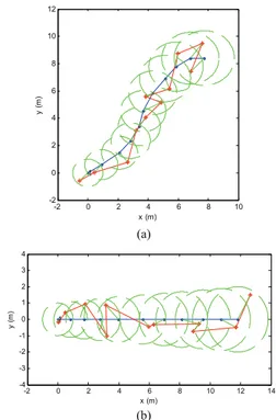
An example of peer movement is illustrated in Fig. 1(a). During 10 seconds, the peer moves using the Random Pedestrian Mobility Model with a mean speed of 1.2 m/s, a standard deviation of the speed of 0.2 m/s and a standard deviation of the direction of /6 (dots). The circles linearly growing over time represent the possible areas in which the estimated positions will be randomly located. The self-estimated position of the peer is plotted with stars and quickly deviates from the exact position.
B. Comparison of Peer Positions and Self-estimated Positions
For simplicity, in Fig. 1(b), the peer is assumed to travel along the positive x direction during 10 seconds. Here we can clearly see how random the variation of the self-estimated positions will be. Even in this case the self-estimated peer trace (star line) generated by the above method still looks considerably random. Obviously, this kind of error variation assumption is not realistic. However, it can be considered in our simulations at least as a possible worst case of how the error changes over time.
C. Simulation Parameters
A simulation is parameterized with the node density, i.e. the number of peer nodes within range , the range corresponding to the RSS threshold ( ), the mean speed of the peers ( ) and the linear error drift rate ( ).
Other less important parameters have been fixed: is set to
1 meter, set to 300 collections (one per second for five minutes). The standard deviation of the peer direction is set to /6 and the standard deviation of the peer speed is set to 0.2 m/s.
Once the parameters have been set, the same simulation is run 50 times with different random seeds to ensure statistical reliability.
(a)
(b)
Fig. 1. Two examples of 10-second trajectory. The dots curve is the trajectory generated with the Random Pedestrian Mobility Model; the stars are positions produced with the linearly drifting error model at every second; the circles bound the scopes where the self-estimations will occur at every second.
IV. SIMULATION RESULTS
In this Section we analyze the results of the simulations carried out with different parameters. We study the impact of each individual parameter on the accuracy of the LMI+barycentric estimation.
A. Preliminary Illustration
Before analyzing in detail the impact of the different parameters on the accuracy of the LMI+barycentric estimation, we illustrate its behavior on a complete example.
The example simulation parameters are set as follow: node density is set to 50 peers within range; range is set to 10 meters; the mean speed of the nodes is set to 1.2 m/s; and the linear error drift rate is set to 0.1 m/s: the self-estimation error bound of each peer node drifts linearly from 1 to 31 meters over the 5 minutes of the simulation. 50 peers in 10m radius is not as overcrowded as it may seem: it is
6 / .
We first look at the performance of the LMI-only estimation during the simulation. In Fig. 2, the LMI-only estimation regular case with peer-self-positioning error (PE) is compared to the LMI-only estimation without PE, where exact peer
-2 0 2 4 6 8 10 -2 0 2 4 6 8 10 12 1 x (m) y ( m ) -2 0 2 4 6 8 10 12 14 -4 -3 -2 -1 0 1 2 3 4 1 x (m) y ( m )
positions are used. The LMI-only estimations without PE all have an error smaller than 2 meters while the LMI-only estimations with PE are comparatively greater (though smaller than 6 meters) because they are based on erroneous self-estimations. The better performance of the LMI-only estimation without PE is further illustrated by Fig. 3, where the error curve of the LMI-only estimation with PE (the noisiest one) is most of the time greater than that of the LMI-only estimation without PE.
(a) (b)
Fig. 2. Spatial distribution of LMI location estimations of the user in polar coordinates. (a) plots the only estimations without PE; (b) plots the LMI-only estimations with PE.
Fig. 3. Variation of the LMI estimation error over time. The lower line is the LMI-only estimation error without PE fluctuating over time; the dashed lower straight line is its mean; the upper line is LMI-only estimation error with PE increasing over time and the dashed upper line is its mean.
Let us now compare the performance of the LMI+barycentric estimations. Fig. 4 illustrates the distribution of LMI+barycentric estimations around the user position: there is no visible difference of performance. This is confirmed in Fig. 5, which illustrates the estimation error for both LMI+barycentric estimations. After barycentric management, the performance of the LMI+barycentric estimation with peer-self-positioning error (PE) is nearly as good as the performance of the estimation without PE, although self-estimations drift all the simulation long.
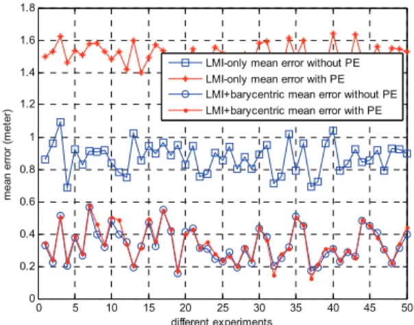
The good performance of the LMI+barycentric estimation with PE was confirmed by running 50 times the same simulation with 50 different random seeds. For each simulation run, we compute the mean of the various types of estimation error over the 5 minutes. Fig. 6 plots these means for each simulation run. In all the experiments the same behavior is confirmed: the LMI-only estimationwithout PE is significantly more accurate than the LMI-only estimation with PE, while the LMI+barycentric estimation without PE is only slightly more accurate than the LMI+barycentric estimation
with PE.
(a) (b)
Fig. 4. Spatial distribution of barycentric location estimations. (a) is the case without PE; (b) is the case with PE.
Fig. 5. Variation of the LMI+Barycentric estimation error over time. The lower line is the LMI+Barycentric estimation error without PE; the dashed lower line is its mean; the upper line is the LMI+Barycentric estimation error with PE and the dashed upper line is its mean.
Fig. 6. Comparing LMI-only and LMI+Barycentric mean errors across 50 simulation runs.
B. Impact of the Simulation Parameters
In this Section we investigate how the variation of parameters , , and affect the performance of the LMI+barycentric estimation. From now on, we only consider the LMI+barycentric estimation with peer-self-positioning error (PE) and do not use the distinction “with PE” anymore. We use the preceding simulation as a basis of comparison.
2 4 6 30 210 60 240 90 270 120 300 150 330 180 0 2 4 6 30 210 60 240 90 270 120 300 150 330 180 0 0 50 100 150 200 250 300 0 1 2 3 4 5 6 Time (sec) E rro r (m et er )
LMI-only estimation error without PE LMI-only estimation error with PE
the case with PE
0.5 1 1.5 2 30 210 60 240 90 270 120 300 150 330 180 0 0.5 1 1.5 2 30 210 60 240 90 270 120 300 150 330 180 0 0 50 100 150 200 250 300 0 0.2 0.4 0.6 0.8 1 1.2 1.4 1.6 1.8 2 Time (sec) B ary ce nt er E rro r (m et er )
LMI+barycenter estimation error without PE LMI+barycenter estimation error with PE
the case with PE
0 5 10 15 20 25 30 35 40 45 50 0 0.2 0.4 0.6 0.8 1 1.2 1.4 1.6 1.8 different experiments m ean e rror ( m et er )
LMI-only mean error without PE LMI-only mean error with PE LMI+barycentric mean error without PE LMI+barycentric mean error with PE
1) Node Density Impact
Different values of the node density parameter ( ) have been investigated. Table I below gives the accuracy of the LMI+barycentric estimation for each investigated value.
Each line of this table and the following tables was produced by running 50 times the simulation with the given set of parameters ( , , , ) but with different random seeds, as for Fig. 8. For each the 50 simulation runs a mean error was computed. The table gives the mean and the standard deviation of these 50 mean errors.
TABLEI
IMPACT OF THE PEER NODE DENSITY ON THE LMI+BARYCENTRIC
ESTIMATION ERROR Mean (m) Std Dev (m) 2 1.84 0.61 4 1.14 0.30 8 0.85 0.29 16 0.61 0.21 50 0.34 0.11 =10m, =1.2m/s, =0.1m/s
Table I shows that to achieve an accuracy of less than 1 meter, 16 peer nodes or more are needed within a range of 10 meters. 4 peer nodes or more within range still allow a good accuracy of less than 2 meters.
The accuracy of the LMI+barycentric estimation increases with the node density. This is because peers have independent errors, and in that case more nodes mean more LMI inequalities and an optimum closer to the real position . However, the impact of this parameter is rather low since good results can be obtained even with only a few nodes.
2) Range Impact
Two values of the range parameter ( ) have been investigated: 10 meters (already in Table I) and 30 meters, which is a rather high value in popular indoors WiFi networks. So we have considered the case of 16 and 50 peer nodes within range, which gave very good accuracy in the previous Section.
Table II below was produced similarly as Table I, i.e. the given means and standard deviations of the LMI+barycentric estimation error are for 50 simulation runs with the same set of parameters but with different random seeds.
TABLEII
IMPACT OF THE RANGE ON THE LMI+BARYCENTRIC ESTIMATION ERROR
(m) Mean (m) Std Dev (m) 16 10 0.61 0.21 16 30 3.26 1.06 50 10 0.34 0.11 50 30 1.90 0.71 =1.2m/s, =0.1m/s
Table II shows that increasing the range highly degrades the accuracy of the estimation. For 16 peer nodes within range, the mean error is higher than 3 meters, and sometimes reaches
5 meters. For 50 peer nodes within range, the accuracy only slightly better: the mean error is almost 2 meters, sometimes reaching 4 meters. This is because the right side of the equation (4) increases and gives a greater intersection for the computation of the optimum. From a geometrical point of view, the greater the intersection is, the more chance the optimum will have to be far away from .
The range parameter has therefore a big impact on the performance, and we should try to keep it low: the accuracy is better with a small range and only a few nodes than with a large range and a lot of nodes. For instance, looking back at Table I, 2 nodes within a 10-meter range outperform 50 nodes within a 30-meter range.
3) Speed Impact
We now investigate the mean peer speed parameter ( ) by considering an alternate speed of 0.6 m/s, i.e. a slow pedestrian. Table III below gives the performance of the LMI+barycentric estimation for 16 and 50 nodes, and with 0.6 m/s and 1.2 m/s speeds. Each line gives the mean and standard deviation of the mean error over 50 simulation runs, as for Tables I and II.
TABLEIII
IMPACT OF THE PEER SPEED ON THE LMI+BARYCENTRIC ESTIMATION ERROR
(m/s) Mean (m) Std Dev (m) 16 0.6 0.97 0.36 16 1.2 0.61 0.21 50 0.6 0.54 0.21 50 1.2 0.34 0.11 =10m, =0.1m/s
Table III shows that decreasing the peer speeds also decreases the accuracy of the estimation. For 16 slow pedestrians within range, the error is almost 1 meter on average, reaching a maximum of 2 meters. For 50 slow pedestrians, the performance is better, the error being 54 cm on average, reaching at worse 1 meter. With slower peers, the consecutive LMI-only estimations are less distributed spatially. This smaller spatial diversity leads to a smaller efficiency of the barycenter computation.
The accuracy therefore increases with the speed. However the impact is rather low on the performance, since good results can be achieved with slow speed.
4) Error Drift Rate Impact
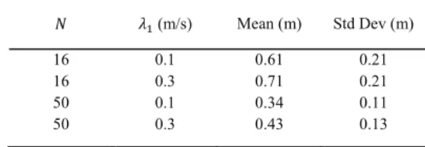
Finally, we investigate the impact of parameter i.e. the error drift rate) on the accuracy of the estimation by considering an alternate value of 0.3 for 16 and 50 peers within range. Table IV below summarizes the results and was produced similarly as Tables I to III with 50 simulation runs per line.
TABLEIV
IMPACT OF THE LINEAR ERROR DRIFT RATE ON THE LMI+BARYCENTRIC
ESTIMATION ERROR (m/s) Mean (m) Std Dev (m) 16 0.1 0.61 0.21 16 0.3 0.71 0.21 50 0.1 0.34 0.11 50 0.3 0.43 0.13 =10m, =1.2m/s
Table IV shows that the increase of the drift rate from 0.1 to 0.3 only slightly degrades the accuracy of the estimation. For 16 peers within range, the mean error changes from 61 cm to 71 cm, and for 50 nodes it changes from 34 cm to 43 cm. These are still very good results. In this case, the accuracy decreases because the increase of also leads to an augmentation of the right side of Equation (4). As in the range impact case, this leads to a larger intersection where the LMI optimum has more chances to be far away from the user position.
The accuracy therefore decreases while the drift rate increases. However the drift rate does not have a strong impact on the estimation accuracy since good results can be achieved with comparatively high values of the rate ( = 0.3 implies an error bound of 90 meters after 5 minutes).
5) Summary
The simulations described above have shown that the accuracy of the raw barycentric location estimation degrades when the amount of nodes within range N decreases, the range threshold increases, the peers mean speed decreases and the error drift rate increases.
The parameter which has the strongest impact on the accuracy is the range threshold. The amount of peer nodes within range also has a moderately strong impact on the accuracy. The peer speed and the error drift rate have a lower impact on the accuracy. Simulations also showed that the best tradeoff is to reduce the threshold range although this also decreases the amount of peer nodes within range.
V. RELATED WORK
At the present time, in the indoors positioning domain, a large number of systems are based on methods measuring distance from several beacon nodes to realize localization, such as AOA (Angle Of Arrival) [5], TOA (Time Of Arrival) or TDOA (Time Difference Of Arrival) [6]. In some special environments, they can reportedly achieve fine-grained positioning precision. However, all of them need specialized equipments either on the beacon nodes or the user side. For example, the AOA systems require a directional antenna featuring beam-forming to estimate the angle of arrival of the received signal, while in terms of TOA and TDOA they generally process some high precise timers to meet the synchronization requirement.
Additionally, because TOA and TDOA supply the distance information by measuring the propagation time of the signals
with high propagation speed, a small measurement error may induce a great distance estimation error. Moreover, multiple paths may also take great effect on the distance measurements from AOA, TOA or TDOA.
Some other existing indoors positioning systems can conquer the multipath effect to some degree, such as the Ubisense location system, which is based on the UWB technology [7] [8]. Though it can achieve accuracy of the order of 15 cm, this system also relies on the use of specialized equipment comprising several UWB base stations and UWB transmitters carried by users. And if there are not enough line-of-sight paths between the transmitters and the receivers then the received signal is strongly attenuated and the accuracy is degraded.
RSS is another widely used method especially for 802.11b-based indoors positioning. This method either measures the distance according to the diminishment state of the radio signal or collect signal strength at different positions to construct a position-relevant RSS radio map[9]. The difficulty lies in the precise measurement of radio signal strength and the precise modeling of the relation between signal strength and propagation distance. A study [10] indicates that all of these RSS algorithms have a common limit that results in a median positioning error of approximately 3 m without more appropriate environment models or additional positioning infrastructure.
In [12][13], a System-on-Chip (SOC) for wireless sensor networking, Texas Instruments CC2431, which is based on RSS trilateration method, claims that an accuracy of better than three meters can be achieved with readout resolution of 0.25m. But the best possible accuracy has a great reliance on the signal environment, the use of special near-isotropic radiation antennas and the optimized deployment of some fixed reference beacon nodes. In [11], an advanced integration of 802.11b equipments and Inertial Navigation System (INS) is used to enhance the performance of the indoor positioning system. As a result, a system performance close to the meter accuracy can be achieved with a low density of access points in the environment provided that users carry inexpensive INS equipment.
All the methods described above require a special infrastructure covering the whole environment for the purpose of precise measurements. Some methods attempt to release these constraints.
In [2] Doherty et al. pioneered the use of semidefinite programming (SDP) methods in the localization problem. The problem is considered as a bounding problem containing several convex geometric constraints mathematically represented as linear matrix inequalities (LMI). The mechanism proposed in this paper is based on this approach, taking into estimation errors and introducing a barycentric improvement over time.
The Centroid localization method [14] is developed to estimate the user’s location by computing the barycenter of all the positions received from fixed beacon nodes. To find the optimum deployment of those beacon nodes for a given application may consume a lot of labor.
In the APIT method [15], a user chooses three beacon nodes around him as the triangle vertex point and uses the APIT algorithm to test if he is lying in the triangle. If the APIT test can be passed, i.e., at least one node’s signal is becoming stronger when the user move towards any direction, the barycenter of the triangle will be taken as the location estimation of the user. Continuously, another different three nodes will be chosen to face the APIT test again. If the new test can also be passed, the barycenter of the intersection of the triangles will be used. By analogy, the user will repeat this APIT test until all combinations are exhausted or the satisfying accuracy is achieved. It is noticeable that since the APIT test is used under the condition of static beacon nodes, accomplishing it is still not an easy thing. Additionally, the APIT test may fail in less than 14% of the cases.
Other research works jointly solve the time synchronization and localization problems. For instance, Enlightness [16] relies on the availability of beacon nodes (at least 5% of the nodes) providing absolute time and space information, like the GPS in outdoor environments. Enlightness combines recursive positioning estimation [17] with a clock offset estimation scheme based on the measure of beacon packet delays and timestamps.
VI. CONCLUSION AND FUTURE WORK
In this paper we have investigated the raw barycentric location estimation, an indoors positioning mechanism that does not involve special equipment or full coverage of the target area and tolerates drifting measurement errors. It is based on the opportunistic exchange of peer location self-estimations.
Our simulations have shown that we could achieve an accuracy of less than one meter under a number of reasonable assumptions concerning the radio range, the peer speeds and the number of peers within range. We have also shown that a linear drift of the self-estimation error could be tolerated. Typically, a user waiting for 5 minutes with 16 peers within a 10 meters range moving a 1.2 m/s and sending self-estimations of their position linearly growing from 1 meter to 31 meters can finally obtain an estimation of its position with accuracy better than 1 meter.
In future work, we will consolidate this work by relaxing a number of assumptions. For instance, we will use more realistic pedestrian mobility models. We will investigate the relationship between the monitored RSS and a maximum distance for WiFi radios. We will introduce more realistic communications such as duty cycles to save energy, and a more realistic communication channel taking into account noise and interferences. We will investigate the case of a moving user. We will define strategies for peers to be able to exhibit linearly drifting self-estimations with periodic reset to a good estimation, for instance using the available infrastructure or manually entering data from a map. Finally, we will investigate the use of a warm-up time to enhance the accuracy of the estimation and/or reduce the user waiting time.
ACKNOWLEDGMENT
The authors would like to thank Emmanuel Conchon, Jérôme Lacan, Yves Caumel, Francesco Zorzi and Andrea Zanella for valuable discussions on this topic.
REFERENCES
[1] G. Kang, T. Pérennou, M. Diaz, “Barycentric Location Estimation for Indoors Localization in Opportunistic Wireless Networks,” to appear in
Proc. of the Second International Conference on Future Generation Communication and Networking (FGCN 2008), Sanya, China, 2008, 6p.
[2] L. Doherty, K. S. J. Pister, and L. E. Ghaoui, “Convex position estimation in wireless sensor networks,” in Proc. of the Twentieth
Annual Joint Conference of the IEEE Computer and Communications Societies (IEEE INFOCOM 2001), Anchorage, USA, 2001, pp.
1655-1663.
[3] L. E. Ghaoui, E. Feron, and V. Balakrishnan, Linear Matrix Inequalities
in System & Control Theory (Studies in Applied Mathematics, Volume 15). Society for Industrial and Applied Mathematics (SIAM), 1994.
[4] The MathWorks, The LMI Lab and Robust Control Toolbox™, [Online] Available: http://www.mathworks.com
[5] D. Niculescu and B. Nath, “VOR base stations for indoor 802.11 positioning,” in Proc. of the Tenth Annual International Conference on
Mobile Computing and Networking (ACM MobiCom 2004),
Philadelphia, USA, 2004, pp. 58-69.
[6] N. B. Priyantha, A. Chakraborty, and H. Balakrishnan, “The Cricket location-support system,” in Proc. of the Sixth Annual International
Conference on Mobile Computing and Networking (ACM MobiCom 2004), Boston, USA, 2000, pp. 32-43.
[7] Ubisense homepage. http://www.ubisense.net
[8] F. Ramirez-Mireles, “On the performance of ultra-wide-band signals in gaussian noise and dense multipath,” IEEE Transactions on Vehicular
Technology, vol. 50, no. 1, pp. 244-249, 2001.
[9] P. Bahl and V. N. Padmanabhan, “Radar: An in-building RF-based user location and tracking system,” in Proc. of the Nineteenth Annual Joint
Conference of the IEEE Computer and Communications Societies (IEEE INFOCOM 2000), Tel Aviv, Israel, 2000, pp. 775-784.
[10] E. Elnahrawy, X. Li, and R. P. Martin, “The limits of localization using signal strength: a comparative study,” in Proc. of the First Annual IEEE
Communications Society Conference on Sensor and Ad Hoc Communications and Networks (IEEE SECON 2004), Santa Clara, USA,
2004, pp. 406-414.
[11] F. Evennou and F. Marx, “Advanced integration of WiFi and Inertial Navigation Systems for Indoor Mobile Positioning,” EURASIP Journal
on Applied Signal Processing, vol. 2006, Article ID 86706, 11 pages,
2006.
[12] Texas Instruments, TI/Chipcon CC2431, "Wireless Sensor Network Zigbee/IEEE 802.15.4 SoC RF Solution with Location Engine", 2006. [13] Geoff V Merrett, Alex S Weddell, Luca Berti, Nick R Harris, Neil M
White and Bashir M Al-Hashimi, “A Wireless Sensor Network for Cleanroom Monitoring”, in Proc. of Eurosensors 2008, Dresden, Germany, Sept. 2008
[14] Nirupama Bulusu, John Heidemann and Deborah Estrin, “GPS-less low cost outdoor localization for very small device”, IEEE Personal
Communications Magazine, 7(5):28-34,October 2000.
[15] Tian He, Chengdu Huang, Brian M. Blum, John A. Stankovic, Tarek Abdelzaher, “Range-free localization schemes for large scale sensor networks”, in Proc. of the Ninth Annual International Conference on
Mobile Computing and Networking (Mobicom 2003), San Diego, USA,
September 2003.
[16] Azzedine Boukerche, Horacio A.B.F. Oliveira, Eduardo F. Nakamura, and Antonio A.F. Loureiro. “Enlightness: An enhanced and lightweight algorithm for time-space localization in Wireless Sensor Networks”, in
Proc. of IEEE Symposium on Computers and Communications (ISCC 2008), Marrakech, Morocco, July 2008, pp. 1182-1189.
[17] Joe Albowicz, Alvin Chen, and Lixia Zhang, “Recursive position estimation in sensor networks”, in Proc. of the 9th International Conference on Network Protocols (ICNP 2001), Riverside, USA,