THE EVOLVING IMPACT OF CONTINENTAL ACCESSIBILITY ON LOCAL EMPLOYMENT GROWTH, 1971-2001 Richard SHEARMUR, Mario POLÈSE, and Philippe APPARICIO
INRS
Urbanisation, Culture et Société
NOVEMBER 2007The Evolving Impact of Continental
Accessibility on Local Employment Growth,
1971-2001
Richard SHEARMUR, Mario POLÈSE, and Philippe APPARICIO
Spatial Analysis and Regional Economics Laboratory (SAREL)
Paper presented at the North American Meetings of the Regional Science Association International,
Savannah, November 7-10, 2007
Institut national de la recherche scientifique Urbanisation, Culture et Société
Richard Shearmur richard.shearmur@ucs.inrs.ca Mario Polèse mario.polese@ucs.inrs.ca Philippe Apparicio philippe.apparicio@ucs.inrs.ca
Inédits, collection dirigée par Mario Polèse :
mario.polese@ucs.inrs.ca
Institut national de la recherche scientifique Urbanisation, Culture et Société
385, rue Sherbrooke Est Montréal (Québec) H2X 1E3
Téléphone : (514) 499-4000 Télécopieur : (514) 499-4065
www.ucs.inrs.ca
The authors would like to thank Infrastructure Canada (Peer Review Research Studies Program) and the Social Sciences and Humanities Research Council of Canada (SSHRC) for their financial assistance. The first two authors are titleholders of Canada Research Chairs, respectively, in Spatial Statistics and Public Policy and in Urban and Regional Studies.
TABLE OF CONTENTS
LIST OF TABLES ... IV
LIST OF FIGURES ... IV
ABSTRACT / RÉSUMÉ ... V
INTRODUCTION ... 1
1. “ACCESSIBILITY” AND REGIONAL GROWTH ... 3
2. METHODOLOGY AND DATA ... 7
2.1 Data ... 7
2.2 The Model ... 8
2.3 Accessibility measures ... 9
3. RESULTS ... 13
3.1 Factor Analysis ... 13
3.2 Accessibility and Location ... 15
3.3 Accessibility and Growth: Results with and without the CPS Model. ... 17
3.4 The Relationship with Employment Growth by Industry and by Modal Mix ... 25
CONCLUSION ... 31
APPENDIX 1 – DETAILED RESULTS ... 33
iv
List of Tables
Table 1 Correlations between the 8 accessibility measures across 359 Canadian regions ... 13
Table 2 Four types of modal mix ... 14
Table 3 Strength (standardised regression coefficient) and Direction of the Relationship between Industry Location Quotients (2001) and Continental Accessibility by Modal
Mix* ... 16
Table 4 Relationship (adjusted r2 increase) Between Continental Accessibility and Employment Growth, 1971-2001: Combined Impact of 4 Modal Mixes ... 27
Table 5 Total employment and Gini coefficient, 2001 ... 28
List of Figures
Figure 1 Evolving Relationship between Continental Accessibility and Total Local Employment Growth, 1971-2001. Direct Relationship (a) and in CPS Model (b). ... 18
Figure 2 Evolving Relationship between Continental Accessibility and Total Local Employment Growth, by Modal Mix, 1971-2001. Direct Relationship (a) and in CPS Model (b) ... 19
Figure 3 Evolving Relationship between Continental Accessibility and Growth in Manufacturing Employment, 1971-2001. Direct Relationship (a) and in CPS Model (b) ... 20
Figure 4 Evolving Relationship between Continental Accessibility and Growth in Manufacturing Employment by Modal Mix, 1971-2001. Direct Relationship (a) and in CPS Model (b) ... 21
Figure 5 Evolving Relationship between Continental Accessibility and Employment Growth in
Producer Services. 1971-2001. Direct Relationship (a) and in CPS Model (b) ... 22
Figure 6 Evolving Relationship between Continental Accessibility and Employment Growth in Producer Services by Modal Mix, 1971-2001. Direct Relationship (a) and in CPS Model (b) ... 23
Abstract / Résumé
Using an econometric model, the paper examines the impact of transport infrastructures (roads, rail, ports, air) – via the accessibility they provide to continental markets – on local employment growth in Canada. The model is applied separately for three time periods between 1971 and 2001. The results show a positive relationship for every transport mode between accessibility and local employment growth. The positive relationship has strengthened over time, most notably for manufacturing employment. The results also show that transport modes do not act in isolation. The strongest – and growing - relationships are those for combinations of road and port access, a reflection of the growing importance of continental markets for local economies.
Keywords: Regional Growth; Transportation; Infrastructures; North America
À l’aide d’un modèle économétrique, ce papier examine l’impact des infrastructures de transport (routes, rail, ports, air) – par l’intermédiaire de l’accès qu’elles procurent aux marchés nord-américains – sur la croissance local de l’emploi au Canada. Les trois décennies, 1971 à 2001, sont analysées séparément. La relation entre accessibilité et croissance est positive pour les quatre modes de transport et s’accroît dans le temps, notamment pour l’emploi manufacturier. Les résultats révèlent, en parallèle, que les modes de transport n’agissent pas de manière isolée. Les relations (positives) les plus fortes – et croissantes – sont celles pour des mixes de transport par routes et par ports de mer, indice de l’importance croissante du commerce intracontinental pour les collectivités canadiennes.
Introduction
The purpose of this paper is twofold. First: to further our understanding of spatial variations in employment growth, specifically the role of transportation infrastructures via the access they provide to markets. Second: to improve our capacity to model regional growth in Canada, building on previous applications (Shearmur and Polèse 2005, 2007). In this respect, a primary contribution of this paper is the introduction into the model of accessibility variables – extremely complex to produce – covering all of North America (US and Canada), which are applied to 145 urban and 214 rural spatial units for Canada below the 55th parallel. The relationship between “accessibility” and growth is examined both directly (without the model) and with the model. Four “accessibilities” are calculated, associated with varying combinations of transport modes: roads and highways; railways, airline networks, and ports. By the same token, the paper presents what we believe is a novel methodology for analyzing the impact of transport infrastructures on local employment growth.
The analysis covers the three decades from 1971 to 2001, a period of accelerating continental integration, notably following the signing in 1989 of the FTA (Free Trade Agreement) between the US and Canada, which later became NAFTA (North American Free Trade Agreement) when Mexico also joined. The share of GDP exported to US markets has risen steadily in all Canadian provinces (Statistics Canada 2000, 2004). Understating how this evolving reality affects regional variations in growth is an additional motivation behind the paper. In Shearmur and Polèse (2007), the authors found that proximity to the US border – using simple North-South coordinates – was positively associated with growth for the two most recent decades. However, this is a crude measure, and tells us nothing about the impact of transport infrastructures or continent-wide market potentials.
An abundant literature exists documenting the positive impact of investments in infrastructures – in transportation infrastructures in particular – on economic growth (Aschauer 1993, Bidder and Smith 1996, Crichfield and McGuire 1997, Freire and Polèse 2003, Kessides 1992, Lobo and Rantisi 1999, Prud’homme 1997). We approach the issue from a different perspective, more closely related to the research tradition of economic geography and regional science. We start with the almost self-evident proposition that the essential characteristic of transportation infrastructures is the accessibility that they provide to other locations across the whole network. The notion of accessibility is at the core of our approach. Our basic postulate, in short, is that “accessibility” – via road, rail, water or air – is a significant determinant of employment growth. We thus begin with a discussion of this multidimensional concept, its possible relationship with local economic growth, and attendant conceptual and analytical issues.
1. “ACCESSIBILITY” AND REGIONAL GROWTH
The term “accessibility” as used here is, in essence, shorthand for other concepts. Access, proximity, and other related concepts that convey the same idea are the cornerstones of economic geography. Access to markets and to inputs – the minimization of transport and spatial interaction costs – is at the core of location theory. However, accessibility is not an easy concept to operationalize, especially when considering various transport modes. Accessibility can take different forms: accessibility in terms of time, cost, reliability of service, etc. A community may have various accessibilities. Thus, a community may be highly “accessible” by road – with a high market potential for goods transported by truck – but with low accessibility for goods transported by water. One would expect such a place to have a different industrial structure – and thus also growth rate – from others with major maritime and/or fluvial infrastructures. Also, different transport modes – and the different accessibilities they provide – are often complements. Selling a good – shipping it by truck or rail – may necessitate several parallel meetings between suppliers and customers, in turn dependant on travel by air or land (passenger) transport. Some “accessibilities” will matter more over shorter distances, while others will matter more over longer distances. Road and air infrastructures do not – for obvious reasons – address the same markets.
Accessibility, clearly, is not the only determinant of growth. The econometric model applied in this paper – presented below – incorporates various variables. The model may reasonably be termed “geo-structural”. Leaving aside the education and wage variables, the variables used refer to size, location, economic structure, and centre-periphery relationships. The model’s conceptual foundations are fairly straightforward. They draw upon the centre-periphery dichotomy (Wallerstein, 1979; Bradfield 1988), agglomeration economies (Marshall, 1890; Phelps and Ozzawa 2003), and the idea that industrial structure and certain other local attributes are determinants of growth. Indeed, numerous writings in economic geography point to the links between growth and agglomeration, industrial diversity, proximity to large urban centres (Fujita and Thisse 2002, Henderson 2003, Krugman 1995, Quigley, 1998), and to the role of industrial specialisation (Porter 1996, 2000), education and increasing returns to human capital (Glaeser 1998, Lucas 1998, Romer 1998, Simon 1998). However, what interests us here is the role “accessibility” plays independently of other factors, for which type of accessibility (which transport mode), and for which industries. We may, for example, reasonably assume that air travel accessibility will be of greater importance for explaining the growth of employment in high-order services – say financial services – than for explaining the growth of manufacturing. The double role of large cities as both points of dense and diverse local interaction and as points of multiple accessibilities (to
4
other points) is an additional analytical problem: there is a circular relationship between agglomeration economies and accessibility, notably for transport modes sensitive to scale economies and the (mainly) service industries that rely on them. The concentration of financial services – to stay with that example – in large cities is undoubtedly driven both by the local density of potential contacts and by the wider accessibility that infrastructures in large urban places provide. It could be argued that accessibility, certainly multi-mode accessibility, is simply a subset of the broader concept of agglomeration economies.
The interdependency between different accessibilities – driven in part by the interrelationship between the production of goods and services – also operates at another level. The concentration of producer services in large cities can affect the location of other industries, in part because the consumption of such (intermediate) services requires face-to-face contacts, a travel cost firms will seek to minimize. Findings for Canada (Polèse and Shearmur 2004, 2006), France (Gaigné et al. 2005) and the US (Desmet and Fafchamps 2005) suggest that manufacturing, specifically medium value-added manufacturing is shifting to small and medium-sized cities, but, within easy reach of larger cities. On the other hand, the search of some manufacturing activities for ever lower cost locations – the automobile and apparel industries are typical examples – may mean that employment, in some cases, will shift to more distant locations (Brülhart 2006, Henderson 1997, Henderson et al 2001). In such cases, the industry is being pulled by at least two accessibilities: towards (but not to) sufficiently large producer service centres; towards continentally accessible – but less costly – locations. In short, we would expect much manufacturing – unless directly tied to resources (i.e. pulp and paper plants) – to be influenced by two distinct accessibilities: accessibility to a large metropolis; accessibility to markets and suppliers, often continental in scope. It is the independent effect of the latter that we wish to isolate.
The interplay between different accessibilities suggests that some transport modes – or mixes thereof – will matter more than others. The road and highway network is by far the most flexible, certainly in North America, generally the first (and often last) leg of any trip. This a priori would tend to favour growth along corridors, traversed by various transport modes, combining the advantages of accessibility to distant markets and to cities located on the corridor. The Economist (2006) notes that of the fifteen new car and truck plants that were opened in the US between 1980 and 1990, all but two were built along Interstates 65 and 75, which form a narrow corridor running from Michigan down the Ohio Valley; since then, three more have been built further south on I-65. Lang and Dhavale (2005) note a similar pattern – for population growth – for other corridors in the US. This is also consistent with the growth of supply chains, where local operations – assembly, tooling, production, etc. –
5
are part of a broader chain of plants and distribution centres.1 A high proportion of Canada-US trade is intra-firm trade. Two major corridors (I-65 and 1-75, between Mobile and Detroit; I-85 and I-95, between Atlanta and Boston) have their northern end-points on or near the Canadian border. The North American automobile industry is largely concentred along an integrated supply chain stretching from Mobile to Oshawa. Wall (2003) finds that some of the strongest increases in Canada-US trade since NAFTA have been between dense industrial regions already fairly well connected, notably between the two central Canadian provinces of Ontario and Quebec and the US Midwest, trade which relies heavily on truckling. We would thus expect continentally calculated accessibility measures for roads and highways to be positively related to employment growth in manufacturing.
We should also expect the attraction of continental market potentials to increase over time – and correspondingly of accessibility to markets – as the requirement for physical proximity to resources diminishes for many manufacturing firms, in addition to the trade effects of NAFTA. A priori, two types of regions should primarily benefit from increased market access: well connected metropolitan areas (Britton 2004) and border regions (Esquival et al. 2003, Helliwell 1998). The growth of global trade – especially over long distances – should in turn favour places with good access to ports and waterways. For the US, Black and Henderson (1999) note the positive growth effects of high market potential and a coastal location; Rappaport and Sachs (2003) observe a general shift of economy activity towards coastal areas, which they explain in part by the continuing (and stable) share of ocean shipping (about on third) in total door-to-door shipping costs.
1
2. METHODOLOGY AND DATA
Our starting point is the local employment growth model developed by Coffey, Shearmur and Polèse (Coffey and Shearmur 1996, Shearmur and Polèse 2005, 2007) henceforth called the CPS model. Its latest version, tested for spatial auto-correlation of residuals, is the base model to which we add accessibility variables. These new variables are designed so that they are independent of one another, as explained below. An increase in explanatory power of the model after including the accessibility variables means that accessibility improves our understanding of employment growth over and above the factors identified by CPS. If the explanatory power of the model remains unchanged, but certain geo-structural variables lose their significance to the benefit of accessibility variables, this would indicate that the geo-structural variables act as (imperfect) proxies for accessibility: in this case once accessibility is explicitly introduced, these variables no longer enter the model significantly.
2.1 Data
Except for the purely geographic data derived from digitized maps of Canada, data used for empirically testing the model are derived from the censuses of 1971, 1981, 1991 and 2001. These data cover 290 census divisions (CDs) and 152 urban agglomerations2 (UAs) which had over 10,000 people in 1991. Since the 290 CDs cover the entire Canadian territory, it has been necessary to manipulate the data in order not to double-count UAs. To do this, data for UAs contained within a CD are subtracted from the CD data, giving data for the UA, and data for the surrounding non-urban area. If a UA overlaps a number of CDs, the CDs are aggregated until there is no overlap.
In this way the database used in the analysis contains 382 distinct regions, 152 urban agglomerations, and 290 rural areas. Because of small employment numbers in far northern regions and of growth dynamics that are specific to northern communities, we have only used 359 regions in the following analysis (145 urban and 214 rural), having excluded all those north of the 55th parallel. In these northern regions we do not expect our growth model to work: low numbers of jobs can lead to erratic growth rates, and the cultural, economic political structures differ greatly from those that can be found in more southern areas of Canada.
2
In fact the database includes the 142 CMAs (Census metropolitan areas) and CAs (Census agglomerations) which had over 10,000 people in 1991, to which were added 10 CSDs (Census sub-divisions) which also had over 10,000 people but were not part of an agglomeration.
8
2.2 The Model
The following regression model is used as a base to which the accessibility measures are added. The reason for proceeding in this way is that the model corresponds to the best achievable without explicitly introducing accessibility. We have previously used it to explore the link between the variables described below and employment growth (g) across the 359 spatial units:
( )
Φ
+
Ω
+
ε
+
=
a
b
c
(
)
g
where g is employment growth over the period analysed,3 Φa vector of 'geo-structural' regional attributes and Ω a vector of local regional attributes.
The geo-structural attributes comprise the X Y coordinates (in degrees), a dummy identifying regions in the Prairies, a series of dummy variables classifying regions into urban central, urban peripheral, rural central and rural peripheral,4 and the logarithm of population. The local attributes comprise the percentage of university graduates in the population 15 years and older, an industrial diversity index (see Shearmur and Polèse, 2005), earned income per employed person and a categorical variable classifying the industrial structure of each region into 8 different types (see also Shearmur & Polèse, 2005). A full description of this model – which is the starting point of our analysis in this paper – can be found in Shearmur and Polèse (2007).
It should be noted that the XY coordinates (particularly the Y coordinate) is interpreted as a proxy for accessibility to the US border in the CPS model. Our new accessibility variables (those that will be added to the CPS model) may be measuring the same thing. However, since there are no multicollinearity problems, and since we are interested in measuring improvements in explanatory power of an existing model, we have left these variables in the regression.
This basic model does not display any heteroskedasticity, there are no outliers (when it is applied to total employment growth) and there is no multicollinearity amongst explanatory variables.
3 Growth between t1 and t2 is measured as (Vt2-Vt1) / Vt1 where Vt is employment at time t. 4
Central urban (agglomeration of over 10,000 people within one hour of an agglomeration of at least 500,000 people),
peripheral urban (other agglomerations of over 10 000 people), central rural (non-urban area within one hour of an
9
2.3 Accessibility measures
The measure of accessibility is at the core of this paper. Broadly speaking, we have conceptualised accessibility as market potential measured along different types of transport network. The exception to this is accessibility to ports: for this type of infrastructure we have assumed that it is accessibility to ports themselves that is important.
Accessibility is measured to the entire North-American market: in other words, accessibility to employment, income and population across North-America. Due to data limitations, we only have North-American wide information (at the county level) for 1990 and 2000. Thus, our accessibility measures were calculated for 1990 and 2000, and for each of the three measures of market. Correlation levels between these three types of accessibility, and between 1990 and 2000, were above 0.99. In other words, despite the population growth and shifts between 1990 and 2000, and despite the fact that the spatial distributions of income, employment and population are not identical, there is almost no shift in relative accessibility between 1990 and 2000.
This should come as no surprise. Despite marginal changes in the spatial distribution of human activity over space, even in the very long term there is considerable inertia in settlement patterns (Davis & Weinstein 2002). In North America since the 1970’s, although changes have occurred, these have not fundamentally altered the pattern of settlement in North America. We have thus used the 2000/2001 accessibility measures for the entire three decades of study.
Accessibility to markets is measured for four each of the four transport infrastructure: roads, railways, air travel and ports. Technical information and data sources relating to the construction of the digitised distance/time networks can be found elsewhere (Apparicio et al. 2007). It should be noted that, except for ports, the three distance matrices indicate the time it takes to travel between two points along the particular transport network.
Road networks: Accessibility along the road network is not constrained by transhipment
costs or by economies over longer distances. We have therefore assumed that, by road, a given local area has access to its own market as well as to all other markets in North America. Thus, for a given local area j, say Montreal for example, accessibility to North American markets is calculated as follows:
∑
= = 1 i b ij i j t M 3500 p if i ≠ j, tij min = 10 minutes. (1)10 b j j j A p a π 5 . 0 = ; Aj min = 1256 km2; Aj max = 11 304 km2 (2) Xj = Mj + aj (3) where
Mj = market potential of j, excluding j; pi = population of i; tij = time between i and j (a
minimum time of 10 minutes is imposed); b = exponent of distance, or distance decay (values used 1 and 2).
aj = auto-potential of j; pj = population of j; Aj = area of j (constrained in order to keep the
denominator between 10 and 30 minutes). Xj = market potential of j
In order to avoid extreme values (due to oddly shaped regions for which the centre of gravity may be outside its boundaries and to some very small regions) a minimum time of 10 minutes has been imposed. For auto-potential (the distance a region is from itself) a maximum time of 30 minutes has also been imposed on the assumption that even within vast sparsely populated regions human activity tends to agglomerate.
Two different values of market accessibility are calculated.
1. The first has a shallow distance decay function (the value of b is 1). With such a value more weight is given to distant markets: it is thus a measure of accessibility that can be considered national or continental.
2. The second has a steep distance decay function (the value of b is 2). With such a value less weight is given to distant markets: it is thus a more local measure of accessibility.
Rail networks: Rail networks are not as all-pervasive as road networks. Railways only go
through certain areas, and some areas are completely inaccessible by railway. We therefore assume that all areas within 200 km of a railway are accessible to it (at a speed of 60 km an hour). The time taken to access the railway, and the time taken at the other end to reach the final destination, is added to the rail time: furthermore, this access time is raised to the power 1.25 in order to take into account the fact that the choice to use a railroad will be more likely the closer one is located to it. Thus, for a region 10 minutes from a railroad, 17.9 minutes are added (101.25). For an area one hour away, 168 minutes are added (601.25). All areas beyond 200 km have no rail access. In Canada, this means that 35 spatial units are deemed to have no
11
rail access. However, given the difficulty in treating these 35 spatial units separately, they are assigned a non-zero accessibility value that is below that of the least accessible spatial unit with rail access. In other words, we treat them as having very low, but non-zero, accessibility to a railway.
Of more importance is the fact that we assume railways are not used to cover distances of less than 200 km. Thus, there is no rail access between areas i and j if the distance of the rail segment between i and j is less than 200 km. Our assumption is that for short distances road transport would be used.
∑
= = n i b ij i j t p M 1 if rail segment of tij >= 200 km (4)n is the number of regions connected to the rail network for which the rail segment of tij is
greater than 200 km. If j is not connected to the rail network (i.e. is over 200 km from the closest railway), then Mj = k. k is a constant inferior to the minimum value of Mj calculated
using formula (4).
Air network: Air transport has been modelled by digitizing all airports in North America.
Airports are categorised, from largest to smallest, into classes 1 to 8. Each type of airport is assigned a transhipment time that takes into account the time necessary to get through security and board, and the time necessary to disembark. It also penalises smaller airports for their lack of connections, and smaller aeroplanes. Only airports linked by direct flights (in 2001) are connected – meaning that in some cases flights are divided into a number of segments (with one time penalty for each break in the flight).
Flight time between airports is estimated by converting distances at the rate of 600 km/hour. These flight times are integrated into an “air and road” matrix; to calculate total time between areas i and j, the following times are summed:
− road time between i and the closest airport − transhipment time at departure airport
− flight time (including transhipment times at stop-over airports) − transhipment time at arrival airport (airport closest to j)
12
The penalties are such that it is never worthwhile to fly over distances that would take less than about 2½ hours by road (this time gets larger the smaller the airports considered). Given the travel times in the “air and road” matrix, accessibility to markets by “air and road” is calculated in exactly the same way as accessibility by road (see formulas (1), (2) and (3)). However, because there is overlap between these road and “air and road” accessibility, we have chosen only to analyse the accessibility that air connections add to road accessibility. Thus air accessibility is defined as the residual, rj, of the following regression:
Mj a= aM j r+b+r j (5) where:
Mja = accessibility by “air and road” calculated applying formulas (1), (2) and (3) using the
“air and road” matrix.
Mjr= accessibility by road calculated applying formulas (1), (2) and (3) using the “road
matrix”
a and b are regression coefficients
rj = residual air accessibility not accounted for by road accessibility.
Ports: Our information on ports is limited.Tonnage breakdown is not available for all ports.
Therefore, we have chosen a simple measure of accessibility for ports. For a region j, accessibility for ports is simply measured as the region's average distance to all 200 ports.
∑
= = 200 1 i b ij j dd , with b set at 1 and 2.
This measure is different in nature from the other three because it does not take into account the spatial distribution of the North-American population. Our assumption is that once goods are loaded onto a ship, distance is largely irrelevant. It is therefore access to ports themselves, and not to markets via ports, which is measured. It should also be noted that this variable is the only one that increases as accessibility decreases. For ease of interpretation we have reversed the signs in the presentation of results.
3. RESULTS
3.1 Factor Analysis
Each of the four types of accessibility has been calculated twice, with distance and distance squared (b= 1 and 2). We therefore have eight different measures of accessibility, many of which are quite highly correlated (Table 1). This correlation is not surprising because, whatever the transport infrastructure along which we choose to calculate accessibility, a remote area will remain remote, and a central one will remain central.
Table 1
Correlations between the 8 accessibility measures across 359 Canadian regions
air_r2 roads1 roads2 rail1 rail2 ports1 ports2 air_r1 0.73 0.00 0.55 0.32 0.48 0.63 0.58 air_r2 -0.36 0.00 -0.02 0.01 0.06 0.01 roads1 0.77 0.43 0.60 0.93 0.88 roads2 0.52 0.75 0.76 0.71 rail1 0.91 0.61 0.60 rail2 0.81 0.78 ports1 0.99
Note: correlations of 0.7 and over are highlighted.
This high inter-correlation poses problems if one is seeking to analyse how these different types of accessibility combine to produce local development results. Therefore, a principal component analysis has been performed on these eight variables. A useful property of the resulting components is that they are not correlated between themselves, making them ideally suited for inclusion in a regression analysis. The results (Table 2) are fairly easy to interpret. Four distinct factors emerge from the analysis, which together explain 98.5% of all variance in continental accessibly between observations (places). In short, four (statistically) independent “accessibilities” exist, each indicative of a unique set of transport modes.
The four dimensions do not simply break down along the lines of the four types of infrastructure used to calculate accessibility. Each component is a composite variable. Henceforth, we shall refer to the four components – 1, 2, 3, 4 – as modal mixes. Each modal mix is characterized by one or two dominant transport modes, which in turn allows us to name them. The fact that each modal mix has an identifiable dominant component means that – at least in terms of accessibility provided – the various transport modes have distinct impacts. Roads do not affect accessibility in exactly the same manner as rail lines, for instance. However, the fact that each is, precisely, a mix signifies that the various modes are
14
not totally disconnected from each other. This is almost self-evident. A harbour without a road leading to it is of little use. The only exception is air accessibility – modal mix 4 – for which one transport mode totally dominates. This is not entirely surprising. Isolated airports can exist, especially in the more peripheral parts of Canada.
Table 2
Four types of modal mix
1. Correlation of each accessibility variable with the four components
C1 C2 C3 C4 Communality air 0.35 0.21 0.69 0.58 96.9% air (time2) -0.02 0.00 0.12 0.99 99.3% road 0.70 0.34 0.60 0.10 97.0% road (time2) 0.43 0.28 0.84 0.14 99.0% rail 0.28 0.94 0.15 0.03 99.2% rail (time2) 0.48 0.77 0.40 0.06 98.2% ports 0.88 0.33 0.34 0.04 99.7% ports (distance2) 0.90 0.32 0.27 0.01 98.8% 2. Variance explained C1 C2 C3 C4 TOTAL Variance 2.68 1.93 1.92 1.35 7.88 % variance 34% 24% 24% 17% 98.5%
3. Contribution of each type of accessibility to each component
C1 C2 C3 C4 air 5% 2% 25% 97% road 25% 10% 55% 2% rail 11% 77% 10% 0% port 59% 11% 10% 0% 4. Component names
C1 Road, port (and rail) accessibility C2 Rail (and road and air) accessibility
C3 Road, continental air (and rail and port) accessibility C4 Regional (and continental) air accessibility
15
3.2 Accessibility and Location
Table 3 gives the strength and the direction of the statistical relation between continental accessibility and location quotients5 for ten industry classes in 2001, with respect to the four accessibility variables. It also gives the total variance – of industry location quotients – explained by the augmented Coffey-Polèse-Shearmur (CPS) model as well as the share explained by the combined impact of the four accessibility variables (last two columns). The ten industries are listed in descending order of the contribution of the four accessibility variables to the explanation of each industry’s location quotient.
To understand how these results should be read, let us at look the results for the primary sector. The standardised regression coefficient for the primary sector on modal mix 3 is 12.5% (strength) with a negative sign (direction); this indicates that local employment specialization in the primary sector is negatively associated with the continental market accessibility provided by the North American road and highway network and airports: for every one standard error increase in Roads (& Air) modal mix there is a 0.125 standard error decrease in the primary sector location quotient. The result is not surprising. We would expect less accessible – smaller and more remote – communities to be more specialized in primary sector activities. No significant relationship exists between the location of employment in the primary sector and the other the three modal mixes. On the other hand, the variables already contained in the CPS model are fairly successful in predicting the location of primary employment, with a total r2 of 60.0, of which only 0.3% is due to the four modal mixes. Primary employment is concentrated in small and peripheral communities (beyond a one hour reach of a major urban areas), two variables already integrated in the model.
On the whole, results in Table 3 are consistent with what one would expect. Wholesaling exhibits the highest positive coefficients for three modal mixes out of four, with rail (modal mix 2) the only exception. It seems entirely logical that distribution and marketing centres should be concentrated in the most accessible locations with the best transport infrastructures and that the four accessibility variables should have a high explanatory power compared to other variables; the opposite of what was observed for the primary sector.
5
The Location Quotient is explained in Appendix 3. The quotient measures the degree to which employment in a particular industry is concentrated in a given community.
Table 3
Strength (standardised regression coefficient) and Direction of the Relationship between Industry Location Quotients (2001) and Continental Accessibility by Modal Mix*
Modal Mix Variance Explained by Model (r2)
Employment in c Harbours (& Roads) d Rail Roads e (& Air) f Airports
(alone) All Variables
4 Accessibility Variables** Wholesaling 41.0% 15.0% 59.6% 29.1% 38.6% 15.7% Public Sector -51.6% -17.5% -45.4% -21.3% 45.5% 11.5% FIRE 24.4% 19.0% 43.8% 43.1% 7.2% Producer Services 40.4% 9.4% 64.3% 5.4% Construction 20.7% 12.8% 41.6% 36.9% 5.3% Manufacturing 17.2% 16.6% 13.4% 54.9% 3.1% Communications 21.3% 37.7% 1.5% Transportation 12.3% 18.0% 0.6% Primary Sector -12.5% 60.0% 0.3% Consumer Services 11.6% 46.3% 0.1%
* Only statistically significant results (90%+) are shown. All four accessibility variables are added to the base model: their standardised regression coefficients are shown here. ** increase in r2 attributed to introduction of the four accessibility variables
Note: The table should be read as follows: for 1 standard error increase in the 'Harbours and Road' component score there is a 0.41 standard error increase in wholesale location quotient.
17
The location of manufacturing employment is positively associated with three of the four modal mixes. In other words, specialization in manufacturing is positively related to continental accessibility. However, no positive statistical relationship exists for modal mix 3 (roads and air). Modal mix 3 is the most closely associated with city size. City size as well as the distinction between close – central – cities and those located beyond an hour’s drive of a major metropolis – peripheral places – is a key element of the CPS model. Manufacturing tends to be relatively concentrated in small and mid-sized cities located within easy travelling distance of major metropolitan areas, which in part is why the four accessibilities contribute so little to the explanation of the location quotient, similar to what was observed for the primary sector, but for the opposite reason (in this case, central locations are favoured). The results on Table 3 do not mean that modal mix 3 is not important for manufacturing, but rather the relationship is mediated via their proximity (or not) to a major city that ranks well on modal mix 3. The relationship between modal mix 3 and city size is highlighted by the coefficients for producer services and for FIRE (Finance, Insurance, and Real Estate), which are positive in both cases. The positive relationship with air accessibility (a component of both modal mix 3 and 4) for producer services is, again, as expected.
Finally, a word is in order on public sector employment, which includes education and health. All the coefficients are negative. In other words, public sector employment plays a countervailing role, counter-balancing the centralizing forces inherent in the search – by firms – for the most accessible locations. Public sector employment is proportionally concentrated in the least accessible places.
3.3 Accessibility and Growth: Results with and without the CPS Model
We now turn to the impact of accessibility on growth. Recall that the base CPS model includes geographic attributes that are also related to continental accessibility: city size (S), proximity (or not) to a major metro area (UC), a regional Prairie dummy (P), and geographic coordinates (X, Y). Thus, the relationship captured by the complete model – described above – is a minimum, so speak, does not capture the “true” impact of accessibility in all its possible dimensions. The fact (or not) that a spatial unit falls within a one-hour travel radius (or not) of a major Canadian metropolitan area is, is for example, already accounted for in the base model. The “incremental” impact that the full model captures – staying with the same example – is that attributable to greater or lesser continental accessibility within the same central or peripheral class of places. If the difference in growth between classes is entirely accounted for by differences in mean continental accessibility, the (UC) class variable will lose its significance and/or a multicollinearity problem will arise.
18
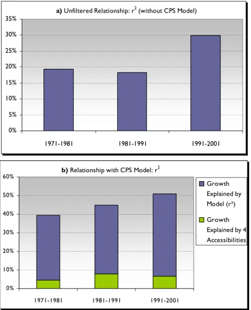
Appendix 1 gives the detailed results for the full CPS model, showing the additional explanatory power attributable to the inclusion for the four accessibility variables in the base model. Thus, taking total employment growth for 1991-2001, the full model explains 44.3% of the variance in local employment growth of which 6.5 percentage points are uniquely attributable to the four accessibility variables – four modal mixes – which thus account for 14.7% of the explanatory power of the model.
a) Unfiltered Relationship: r2 (without CPS Model)
0% 5% 10% 15% 20% 25% 30% 35% 1971-1981 1981-1991 1991-2001
b) Relationship with CPS Model: r2
0% 10% 20% 30% 40% 50% 60% 1971-1981 1981-1991 1991-2001 Growth Explained by Model (r²) Growth Explained by 4 Accessibilities
Figure 1 — Evolving Relationship between Continental Accessibility
and Total Local Employment Growth, 1971-2001. Direct Relationship (a) and in CPS Model (b)6
6
Shearmur and Polèse (2007) report the model's r2, not the adjusted r2. This accounts for the discrepancies between the r2 reported here and that reported in Shearmur and Polèse (2007).
19
a) Unfiltered Relationship: r2 (without CPS Model) by Modal Mix
-40% -30% -20% -10% 0% 10% 20% 30% 40% 50% 60%
Harbours (& Roads) Rail Roads (& Air) Airports (alone) 1971-1981 1981-1991 1991-2001
b) Relationship with CPS Model: Standardized Coefficient by Modal Mix
-10% 0% 10% 20% 30% 40% 50% 60%
Harbours (& Roads) Rail Roads (& Air) Airports (alone) 1971-1981 1981-1991 1991-2001
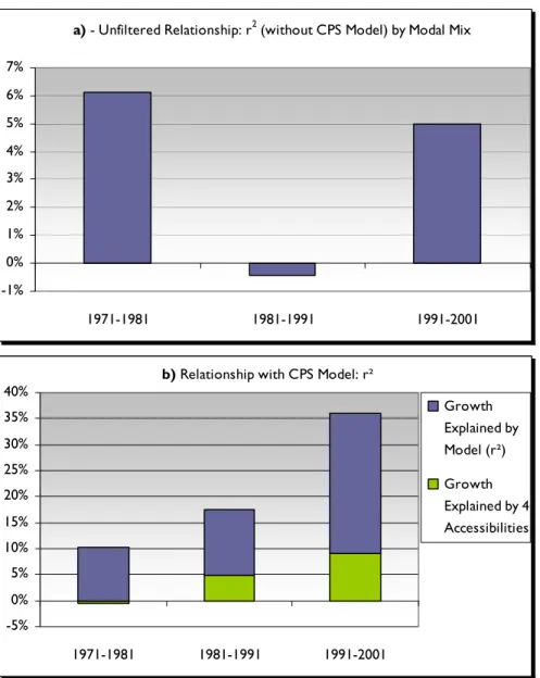
Figure 2 — Evolving Relationship between Continental Accessibility
and Total Local Employment Growth, by Modal Mix, 1971-2001. Direct Relationship (a) and in CPS Model (b)
20
a) - Unfiltered Relationship: r2 (without CPS Model) by Modal Mix
-1% 0% 1% 2% 3% 4% 5% 6% 7% 1971-1981 1981-1991 1991-2001
b) Relationship with CPS Model: r²
-5% 0% 5% 10% 15% 20% 25% 30% 35% 40% 1971-1981 1981-1991 1991-2001 Growth Explained by Model (r²) Growth Explained by 4 Accessibilities
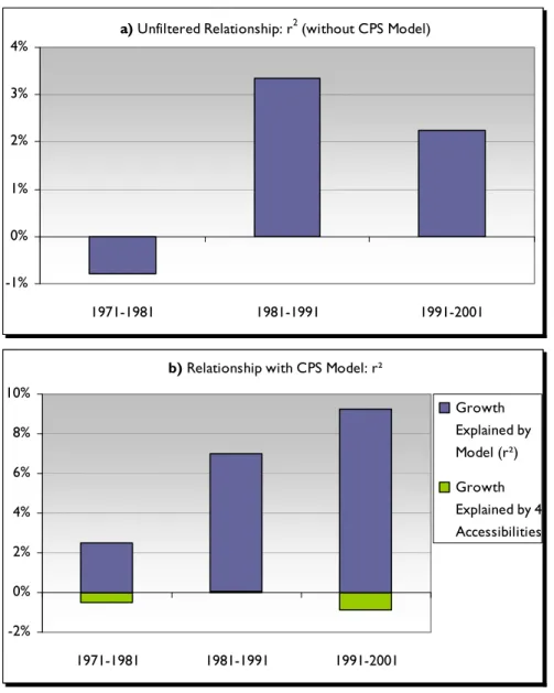
Figure 3 — Evolving Relationship between Continental Accessibility
and Growth in Manufacturing Employment, 1971-2001. Direct Relationship (a) and in CPS Model (b)
21
a) Unfiltered Relationship: Standardized Coefficient (without CPS Model) by Modal Mix
-30% -20% -10% 0% 10% 20% 30%
Harbours (& Roads) Rail Roads (& Air) Airports (alone) 1971-1981 1981-1991 1991-2001
b) Relationship with CPS Model: Standardized Coefficient by Modal Mix
-10% 0% 10% 20% 30% 40% 50% 60%
Harbours (& Roads) Rail Roads (& Air) Airports (alone) 1971-1981 1981-1991 1991-2001
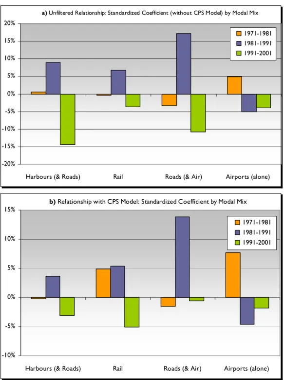
Figure 4 — Evolving Relationship between Continental Accessibility
and Growth in Manufacturing Employment by Modal Mix, 1971-2001. Direct Relationship (a) and in CPS Model (b)
22
a) Unfiltered Relationship: r2 (without CPS Model)
-1% 0% 1% 2% 3% 4% 1971-1981 1981-1991 1991-2001 b) Relationship with CPS Model: r²
-2% 0% 2% 4% 6% 8% 10% 1971-1981 1981-1991 1991-2001 Growth Explained by Model (r²) Growth Explained by 4 Accessibilities
Figure 5 — Evolving Relationship between Continental Accessibility
and Employment Growth in Producer Services. 1971-2001. Direct Relationship (a) and in CPS Model (b)
23
a) Unfiltered Relationship: Standardized Coefficient (without CPS Model) by Modal Mix
-20% -15% -10% -5% 0% 5% 10% 15% 20%
Harbours (& Roads) Rail Roads (& Air) Airports (alone) 1971-1981 1981-1991 1991-2001
b) Relationship with CPS Model: Standardized Coefficient by Modal Mix
-10% -5% 0% 5% 10% 15%
Harbours (& Roads) Rail Roads (& Air) Airports (alone) 1971-1981 1981-1991 1991-2001
Figure 6 — Evolving Relationship between Continental Accessibility
and Employment Growth in Producer Services by Modal Mix, 1971-2001. Direct Relationship (a) and in CPS Model (b)
24
To illustrate the workings of the model, regression results – without the model – between employment growth and the accessibility variables are also shown for total employment, manufacturing, and producer services (Figures 1 through 6). In each of the three cases, the inclusion of the variables contained in the base CPS model significantly alters the relationship between the accessibility variables and local employment growth. But, contrary to what one might expect, the CPS model does not necessarily reduce the (positive) relationship between the accessibility variables and growth. The straight unfiltered relationship – without the model – between continental accessibility (four modes combined) and total employment growth is positive, as one would expect (Figure 1a). This holds for all three periods from 1971 to 2001. However – this is the important finding – the positive impact does not disappear once other variables are added in (Figure 1b). The fact that the relative weight of the incremental impact has declined somewhat over the last period (1991-2001), while the total explanatory power of the model has grown, means that other variables – for example the centre-periphery split between places close to and far from big cities – have grown in importance as determinants of local employment growth. More revealing still is the comparative strength of the relationship with each of the four modal mixes (Figure 2a and b). Looking at modal mix 1 (harbours and roads), the straight, unfiltered, results suggest a negative or negligible impact on growth: there is a strong regional pattern to this variable (western and eastern Canada have low accessibility, central Canada high accessibility) that is not connected to employment growth. However, once this regional effect is filtered out the impact of ports on growth becomes positive (as well as statistically significant in the latter two time periods).
For roads (and airports) – modal mix 3 – the addition of other variables tends to consolidate and even increase the positive impact on growth. For airports (alone) – modal mix 4 – the addition of other variables tends to reverse the signs from negative to positive, as in the case of harbours (though never statistically significant). The explanation is undoubtedly of a similar nature. One would not expect places whose sole or principal accessibility is by air – generally isolated communities – to be terribly dynamic, though they seem to be marginally more dynamic than similar places which lack such access. Not only does this serve to remind us that air accessibility per se – if not also associated with other infrastructure – does not guarantee growth, but also that the impact of transport infrastructures can be different in different settings.
The results for manufacturing are even stronger (Figure 3). The direct regression – without the model – for the combined impact of the four accessibility variables shows a positive relationship with employment growth for two of the three periods (Figure 3a). But, the portrait changes considerably once the model is introduced. The positive relationship with accessibility increases systematically over the three time periods (Figure 3b). Equally, when moving from
25
the direct regression to the model (Figure 4a and b), the results improve noticeably, especially for modal mixes 1 and 3 (harbours and roads; roads and air). The strength of the relationship for roads and air is not statistically significant in the first case (for any time period), but becomes so once other factors are accounted for by the model; the strength of the relationship with ports is much stronger (and growing) in the latter case than the former.
Producer services provide a good illustration of how the augmented CPS model works to factor out elements which can lead to erroneous interpretations (Figures 5 and 6). With the model, none of the results are statistically significant. Indeed, for producer service employment growth, the contribution of accessibility to the explanatory power of the model is negative: adding these variables to the model merely decreases the model's power relative to the number of explanatory variables. The direct regressions, however, suggest a positive relationship since 1981 (Figure 5a) as well as significant relationships – both negative and positive – for modal mixes 1 and 3 (Figure 6a).What the direct regressions mainly capture in this case is the impact of city size; naturally, bigger cities will generally rank higher on the four accessibility variables, especially those related to road and air transport. A positive direct relationship with employment growth (since 1981) is unsurprising. But, this is different from measuring the “independent” impact of accessibility, given city size. Once city size and proximity to a metropolitan area are included, the relationship disappears. The sharp turnaround for the direct regressions after 1991 – making for a negative relationship – for modal mixes 1 and 3 can in part be explained by the 1989 real estate slump, which chiefly affected the largest cities (especially Toronto) and hit the producer service and financial sectors the hardest. The negative relationships pictured on Figure 6a are not necessarily picking up the impact of accessibility, but rather of other factors, notably city size, since the relationship ceases to be significant once city size is introduced. Producer services also provide a useful illustration of the difference between explaining location and explaining growth. The CPS model is quite successful in explaining producer service location, but much less so for growth.
3.4 The Relationship with Employment Growth by Industry and by Modal Mix
The most striking results are those for total employment and for manufacturing, especially as they relate to modal mix 1 (harbours and roads) and modal mix 3 (roads and air). It is worth taking a second look at Figures 1b and 3b. For total employment, the augmented CPS model is surprisingly successful in explaining growth: an adjusted r2 of 44.3% for 1991–2001. Its explanatory power has grown over time, which suggests, that the variables contained in the model are increasingly important as determinants of local employment growth. In addition to the centre-periphery split – which favours places close to big cities – this suggests that city size per se increasingly matters.
26
Equally striking for total employment is the growing strength of the positive relationship with modal mix 1 (harbours and roads) and with modal mix 3 (roads and air). Rail also becomes significant in the last period. In short, continental accessibly, whether by water, roads, rail or air is – it would seem – becoming increasingly important as a determinant of local employment growth. Another way of saying the same thing is that relative location is more – not less – important today than thirty years ago. The results on Figures 1 and 2 – notably as they relate to the road and highway network – suggest that it is not only increased Canada-US trade as such that is at play, but also the geographical pattern of that trade. Truck transport is most cost-efficient and practical for non-bulk trade over short and middle-range distances (up to approximately a 1,000 km, although this varies greatly with circumstances) and for goods that need to be delivered to customized and time-sensitive markets. The growing importance of road accessibility is consistent with the growth of cross-border trade between neighbouring states and provinces.
The growing importance of (continentally calculated) road accessibility should come as no surprise given the growth in Canada-US trade. Earlier, we noted the role of supply chains and of trade corridors, which in the United States generally follow the contours of Interstate Highways. The results for manufacturing on Figures 3b and 4b are consistent with this interpretation. Growth in manufacturing employment has been highest in recent times in places which exhibit the highest continental market potentials – as defined by combined harbour, air and road accessibility. The signs are negative for modal mixes 1 and 3 during the 1970’s when much manufacturing in Canada was still resource-related (sawmills, smelting, fish processing, etc.) and less oriented to US markets. However, the signs become positive in the following decade, growing in strength in the 1990’s for modal mix 1, but decreasing slightly for modal mix 3. The results for modal mix 1 suggest that it is the combination of harbours and roads which is increasingly a crucial factor. The relationship between international trade and harbours is self evident. As trade grows so does the importance of ports and, of course, of the road networks into which they are linked. The statistically non significant result for modal mix 2 (where rail is the predominant mode) is consistent with our comments on the role of highway-based trade corridors. In Canada, this would tend to favour – for manufacturing growth – small and mid-sized cities in Southern Ontario and in Southern Quebec, not too far from Toronto or Montreal, situated on highways leading to US markets and trade corridors, consistent with the findings of Wall (2003) on the changing patterns of US-Canada trade. The role of rail should not be ignored, however. It is useful to recall that modal mixes 1 and 3 also contain rail components.
Summary results by industry – growth explained by the four combined accessibilities – are shown on Table 4. The relatively low values for most industry classes should come as no
27
surprise. Statistically explaining local growth is notoriously difficult at a detailed industry level, where industry-specific and accidental factors increasingly enter into play. A comparison between the explanatory power – by industry – of the model for location (Table 3) and for growth provides a good illustration of the difficulties of explaining growth. The model is systematically more successful in explaining location. Nonetheless, all relationships – save for producer services – are positive. Continental accessibility, in short, is positively related to employment growth for (almost) all sectors of the economy to various degrees.
Table 4
Relationship (adjusted r2 increase) Between Continental Accessibility and Employment Growth, 1971-2001: Combined Impact of 4 Modal Mixes
1971-1981 1981-1991 1991-2001 Primary Sector 0.08% 1.46% 0.71% Manufacturing -0.5% 4.8% 9.1% Consumer Services 6.0% 5.6% 2.6% Producer Services -0.5% 0.1% -0.9% Construction 5.7% 3.3% 0.3% Transportation 5.5% 2.4% 0.7% Communications 11.7% 3.2% 1.1% Public Sector 10.5% 0.2% 9.8% Wholesaling 3.6% 5.5% 0.4% FIRE 2.9% 5.6% 0.4%
Note: This table presents the increase in adjusted r2 attributable to the 4 accessibility variables combined. In some cases, due to the negligible impact of accessibility and the increase in degrees of freedom taken by the model, the adjusted r2 slightly decreases. Of course, the unadjusted r2 can only increase when extra variables are added.
The results in Table 4 suggest that the impact of accessibility on growth in most sectors is declining over time although it is remaining stable overall and increasing for manufacturing. These results reflect a number of interrelated factors. First, in some sectors, the role of the centrality variables is increasing as the role of accessibility decreases: proximity to a metropolitan area is an increasingly good proxy for accessibility. This shows that the scale at which accessibility has an effect is evolving: in some sectors it is no longer better accessibility within a given type of region that is associated with growth (eg: some peripheral regions are more accessible than other peripheral regions), but the fact of being in a type of region that has better accessibility (eg: central as opposed to peripheral). Second, it should be noted that the model has increasing explanatory power for total employment (see appendix 1) even as its explanatory power is decreasing in many sectors. This suggest that there is complex interplay between local growth in individual sectors: overall employment growth in
28
a particular locality may be associated with decline in one sector (say wholesaling) and increase in another (say construction). Thus employment growth of specific sectors may be disconnected from total employment growth, and, in particular, it may be disconnected from accessibility measures. Finally, as the economy is subdivided into sectors employment for some sectors in some localities can get very small. Although all our models are corrected for outliers, the fact remains that there is more noise in our sectoral growth rates than in our overall model.7 The model performs best for the largest sectors – total employment, manufacturing, consumer services and public services (Table 5).
Table 5
Total employment and Gini coefficient, 2001
Jobs Gini Primary Sector 666 380 0.43 Manufacturing 2 079 920 0.62 Consumer Services 4 559 850 0.64 Producer Services 947 995 0.79 Construction 795 160 0.60 Transportation 618 125 0.62 Communications 482 645 0.75 Public Sector 3 345 915 0.63 Wholesaling 666 380 0.71 FIRE 821 815 0.75 TOTAL 14 984 185 0.63
Note: the Gini coefficient measures the % of jobs that would need to be re-allocated in order to obtain an identical percentage of jobs in each of the 359 localities under study. The higher the value, the more jobs are concentrated in a small number of localities (and hence the more likely it is to find small numbers of jobs in many localities).
Over time – for the three decades studied – the results for manufacturing are the most systematic, the explanatory power of continental accessibility rising sharply between 1971 and 2001. As noted earlier, the growing sensitivity of manufacturing jobs to continental accessibility is consistent with changing trade patterns. The products – goods and services – of most other industries (the primary sector excluded) are not continentally traded, at least not massively. In many Canadian localities employment growth is an indirect – induced – effect of growth in manufacturing (or primary exports). The other sector which shows a positive relationship with modal mixes 1 and 3 for the most recent periods is consumer
7
The growth rate is calculated as (Et-Et-1)/Et-1. If Et-1 is very small, then inordinately large rates can be observed even for modest values of Et. The larger the sector analysed, and the more evenly distributed across our 359 regions, the less this matters. FIRE and high-order services are the two most spatially concentrated sectors that we analyse.
29
services, of which retailing is the primary component. These are truly induced activities, generated by growth elsewhere in the local economy. Consumer services largely follow the general trend, with results that are not all that different from those for total employment. By the same token, this is the sector for which the full CPS model is the most successful, with an explanatory power of 44.3% in 1991-2001, the same as for total employment. The decreasing independent impact of accessibility on growth in consumer services is strongly connected with faster growth of these services in (accessible) central areas and with the increasing relevance of the industrial structure classification (which itself reflects a geographic structure that is to some extent linked to accessibility).
The lack of a significant relationship with producer services over the whole period plus the disappearance in 1991-2001 of a statistically significant relationship with FIRE (finance, insurance, and real estate) cannot be attributed to the interplay between accessibility and centrality variables. It is worth recalling that it is the relationship with growth in employment that is being analyzed. Once this is understood, the results for FIRE and for producer services are less surprising. These high-order services were already, in 1971, concentrated in places with high road and air accessibility potentials – the largest urban centres. As tertiarisation diffuses across Canada, higher growth rates are observed in smaller localities. The growth rates themselves are closely related to the number of high order service jobs in the base year, some high growth rates being attributable to the quasi-absence of such jobs. The noise introduced by these random growth rates – particularly evident in the spatially concentrated high-order services (Table 5) but observable in most other sectors also – weakens the model for some sectors.
For the FIRE sector, the disappearance of a statistically significant relationship after 1991 (for modal mixes 1, 2, and 3: Appendix) can be partly explained by the 1989 real estate and financial collapse, alluded to earlier. The composite positive relationship between accessibility and employment growth in FIRE all but disappeared during the same period with a parallel reduction of the explanatory power of the CPS model. Employment growth in the financial sector was slow during most of the 1990s, notably in the traditional large metropolitan centres of finance and corporate control.
Growth in public service jobs is strongly connected to accessibility in the 1970s and 1990s, but not in the 1980s. In the 1970's public sector jobs grew in northern localities distant from ports, yet with high air accessibility: in short they grew fastest in the most accessible parts of remote regions, probably in the smaller central places serving Canada's fast developing resource regions.. The 1980s was a period of change. Rapid growth in resource regions had come to a halt, but public services continued growing there. They also grew at similar rates in more continentally accessible areas: there was no spatial logic to this growth, which is
30
reflected in the low explanatory power of our accessibility variables in the 1980s, and indeed the model's poor performance for this sector over this period (appendix 1). The early 1990s saw massive job cut-backs in the public sector, followed by slow growth towards the end of the decade. Notwithstanding the tendency for public service jobs to be more highly concentrated in remote locations (Table 3), it is evident that the localities best able to retain (and enhance) their public service jobs in the 1990s are the most highly accessible ones. It therefore appears that public sector jobs are no longer compensating for the lack of economic activity in inaccessible regions, but are increasingly contributing to (or accompanying) their decline.
Conclusion
In this paper, we have explored the relationship between continent-wide accessibility and local employment growth for 359 spatial units covering all of Canada below the 55th parallel.
Accessibility variables are devised for four transport mode combinations, involving the digitalisation of North America’s rail, air, and road networks and the introduction of hypotheses relating to the way in which each network is used. Separate regressions are run for total employment growth and for employment growth in ten industry classes for three consecutive decades between 1971 and 2001. The relationship with local employment growth is examined both directly and by introducing the accessibility variables into a broader regional growth model, which includes other variables commonly associated with growth. In almost all cases, the introduction of the four continental accessibility variables adds to the explanatory power of the model. Indeed, our results suggest that the independent effects of continental accessibility on local employment growth – once other factors (including city size and proximity to a large city) have been accounted for – are sometimes greater than what a simple direct relationship would suggest.
The strongest positive relationships with continental accessibility are for total employment growth and for employment growth in manufacturing. Accessibilities associated with the continental road and highway networks exhibit the strongest relationship with total employment growth, with harbours and airports as accompanying modes. For manufacturing employment, accessibilities related to harbours exhibit the strongest positive relationship with growth, notably during the most recent decade. The strength of the positive relationship between continental accessibility (all modes combined) and growth has increased over time for manufacturing. The increase (in explanatory power) is most marked for accessibilities associated with harbours, which is consistent with studies – for the US – that have observed the positive impact of a coastal location on growth.
The independent impact of continental accessibility on growth is not negligible. For manufacturing employment, the introduction of accessibility variables raises the explanatory power of the model by more than a third for 1991-2001. All modal combinations – save solitary air access – exhibit a strong positive relationship with manufacturing employment growth. For this sector it really does seem to matter – independently of other factors – whether a place is well-connected by road, rail, and water to the rest of North America, certainly since the 1990’s. For total employment growth, the addition of the four accessibilities raises the explanatory power of the model by some 15% for the most recent decade (down from about 22% during the previous decade). However, the overall
32
explanatory power of the model has increased over time, a reflection of the increased contributions of other variables such as industrial structure, centre-periphery and rural-urban. Our results suggest that two broad spatial processes are at work, shaping the economic geography of Canada and, arguably, all of North America. First, as economic integration progresses, both continentally and globally, as (longer distance) exports account for an ever growing share of local economies, so the importance of continental and global accessibility will grow. In short, location is becoming more – not less – important. This is not good news for peripheral or sparsely settled.
APPENDIX 1 – DETAILED RESULTS
Relationship between Continental Accessibility and Employment Growth. By Industry and by Accessibility (Modal Mix). Three Periods
The first set of rows under each industry heading shows the strength (standardized regression coefficient) and the direction of the relationship for each modal mix. The second set of rows refers: (a) to the combined impact of the 4 modal mixes and (b) of all variables (in the CPS Model) on employment growth, and (c) to % contribution of the former to the latter.
1971-1981 1981-1991 1991-2001
Total Employment
1. Harbours (& Roads) 0.03 0.15** 0.24**
2. Rail 0.03 0.05 0.09*
3. Roads (& Air) 0.39** 0.51** 0.51**
4. Airports (alone) 0.08 -0.01 0.07
a) Growth Explained by Four Accessibilities (r2) 4.6% 8.0% 6.5%
b) Growth Explained by Complete CPS Model (r2) 34.7% 36.8% 44.3%
c) Contribution of Four Accessibilities as a %
Growth Explained 13.2% 21.7% 14.7%
Primary
1. Harbours (& Roads) 0.00 -0.10 -0.03
2. Rail 0.06 0.06 0.03
3. Roads (& Air) 0.14 0.16 0.21*
4. Airports (alone) 0.10 -0.03 0.07
a) Growth Explained by Four Accessibilities (r2) 0.08% 1.46% 0.71%
b) Growth Explained by Complete CPS Model (r2) 12.72% 10.58% 5.05%
c) Contribution of Four Accessibilities as a %
Growth Explained 0.63% 13.80% 14.06%
Manufacturing
1. Harbours (& Roads) -0.09 0.19** 0.49**
2. Rail -0.04 0.07 0.05
3. Roads (& Air) 0.00 0.47** 0.35**
4. Airports (alone) -0.06 0.09 0.04
a) Growth Explained by Four Accessibilities (r2) -0.5% 4.8% 9.1%
b) Growth Explained by Complete CPS Model (r2) 10.3% 12.8% 26.9%
c) Contribution of Four Accessibilities as a %
Growth Explained -4.8% 37.3% 33.8%
Consumer Services
1. Harbours (& Roads) -0.08 0.03 0.17**
2. Rail -0.05 0.03 0.03
3. Roads (& Air) 0.32** 0.40** 0.35**