HAL Id: hal-02923861
https://hal.archives-ouvertes.fr/hal-02923861
Submitted on 28 Oct 2020
HAL is a multi-disciplinary open access
archive for the deposit and dissemination of
sci-entific research documents, whether they are
pub-lished or not. The documents may come from
teaching and research institutions in France or
abroad, or from public or private research centers.
L’archive ouverte pluridisciplinaire HAL, est
destinée au dépôt et à la diffusion de documents
scientifiques de niveau recherche, publiés ou non,
émanant des établissements d’enseignement et de
recherche français ou étrangers, des laboratoires
publics ou privés.
Inverse modeling of annual atmospheric CO 2 sources
and sinks: 2. Sensitivity study
P. Bousquet, P. Peylin, P. Ciais, M. Ramonet, P. Monfray
To cite this version:
P. Bousquet, P. Peylin, P. Ciais, M. Ramonet, P. Monfray. Inverse modeling of annual atmospheric CO
2 sources and sinks: 2. Sensitivity study. Journal of Geophysical Research: Atmospheres, American
Geophysical Union, 1999, 104 (D21), pp.26179-26193. �10.1029/1999JD900341�. �hal-02923861�
JOURNAL OF GEOPHYSICAL RESEARCH, VOL. 104, NO. D21, PAGES 26,179-26,193, NOVEMBER 20, 1999
Inverse modeling of annual atmospheric CO2 sources and sinks
2. Sensitivity study
P. Bousquet,
• P. Peylin, P. Ciais, M. Ramonet, and P. Monfray
Laboratoire des Sciences du Climat et de l'Environnement, Gif sur Yvette, FranceAbstract. Atmospheric
transport
models can be used to infer surface
fluxes of atmospheric
CO2
from observed
concentrations
using inverse
methods.
One of the main problem of these
methods
is the question
of their sensivity
to all the parameters
involved in the calculation.
In this paper
we study
precisely
the influence
of the main parameters
on the net CO2 fluxes inferred
by an
annual
Bayesian
three-dimensional
(3-D) inversion
of atmospheric
CO2 monthly
concentrations.
This inversion
is described
as the control inversion
(So) of Bousquet
et al. [this issue].
Successively,
at regional
to global spatial scales
we analyze
the numerical
stability of the
solution
to initial fluxes and errors, the influence of a priori flux scenario,
the sensitivity
to the
atmospheric
transport
model
used,
the influence
of/5•3C
measurements,
and the influence
of the
atmospheric
network.
We find that the atmospheric
transport
model introduces
a large
uncertainty
to the inferred
budget,
which overcomes
our control
run uncertainties.
The effects of
vertical transport
on CO2 concentrations
appear
to be a critical point that has to be investigated
further. Spatial patterns
of fluxes also have significant
influence
on a regional basis.
We notice
that accounting
for the Baltic Sea station
(BAL) deeply modifies
the Europe versus
Asia
partition
of the land uptake
at mid and high latitudes
of the Northern
Hemisphere.
We also
analyze
the weak influence
of using/5•3C
measurements
as additional
constraints.
In the tropics
we find that the low level of constraints
imposed
by the atmospheric
network limits the analysis
of fluxes to zonal means.
Finally, we calculate
overall estimates
of CO2 net sources
and sinks at
continental
scale, accounting
for all sensivity
tests.
Concerning
the controversial
partition of
CO2 sink at mid and high latitudes
of the Northern Hemisphere,
we find (on average,
for the
1985-1995
period)
an overall
partition
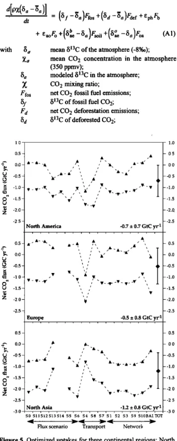
of the sink of 0.7+0.7 Gt C yr -• for North America,
0.2+0.3 Gt C yr -• for the North Pacific
Ocean,
0.5+0.8 Gt C yr --• for Europe,
0.7+0.3 Gt C yr '•
for the North Atlantic
Ocean,
and 1.2+0.8
Gt C yr 4 for north
Asia. This overall
partition
tends
to
place an important
land uptake
over north Asia. However, uncertainties
remain large when we
account
for all the sensitivity
tests.
1. Introduction
Global atmospheric observations of CO2 concentration in the atmosphere can be converted into net surface fluxes by using atmospheric transport models. In order to determine a set of surface fluxes that best matches the atmospheric measurements, inverse methodologies are currently being used [Enting et al.,
1995; Ciais et al., 1995a, Hein et al., 1996; Rayner et al., 1997]. Inversions are based on mass balance calculations [Law et al., 1996; Bousquet et al., 1996] or are of synthesis type [Enting et al., 1993]. Bousquet et al. [this issue] use the latter approach in order to calculate the CO2 fluxes exchanged over 11 continental regions and 8 ocean regions of the globe. Briefly, for each type of source involved in the CO2 budget we establish a global map of a priori fluxes on a monthly basis. The sources (or sinks) are fossil fuel emissions (FOS), land use changes (DEF), land gross primary production (GPP), land total respiration (RES), land net uptake (BIO_UPT), and net ocean fluxes (OCE). Each type of
I Also at Universit6 de Versailles Saint Quentin en Yvelines, Versailles, France
Copyright 1999 by the American Geophysical Union. Paper number 1999JD900341.
0148-0227/99/1999JD900341 $09.00
source is divided into several source regions over the entire globe
which thus determines the source base functions. Note that for land areas the number of source base functions is 3 times the number of source regions because we have three spatial and temporal patterns representing continental exchanges (GPP, RES, and BIO_UPT). The model response for each source base function is computed with the TM2 three-dimensional model [Heimann, 1995]. The Bayesian inverse method optimizes annual source strengths using assumptions on (1) an a priori set of monthly fluxes and errors, (2) the model responses for each source base function, and (3) the monthly atmospheric measurements and errors that are being assimilated to constrain the sources and the sinks regionally.
In this paper we examine how robust the inferred fluxes of our control inversion (So) are to these three types of assumptions in the inverse procedure. To do so, first, we perform a detailed sensitivity analysis to the a priori settings. This includes a sensitivity analysis of the inversion to the initial source strengths and initial errors on the sources prescribed to the model. We also study the way to choose different a priori geographical patterns of emission versus uptake within a given source region and how the increase or decrease the number of regions does impact the inferred sources magnitudes. Second, we address the effect of using another transport model (the TM3 model) instead of the TM2 model in the inverse procedure. This test of atmospheric transport is particularly important since model intercomparisons
26,180 BOUSQUET ET AL.' SENSITIVITY STUDY OF INVERSE MODELING OF CO 2
have already revealed potentially large differences in the CO2 concentration fields that are simulated by different transport codes, highlighting, among others, strong interactions between the seasonal variability of vertical mixing and of land biospheric emissions [Denning et al., 1995, 1997]. Third, we evaluate the specific constraints that are added to the inferred fluxes when
13C/12C
isotope
ratio measurements
are included
in addition
to
CO2 concentration measurements. Also, the specific influence of using in the inversion the CO2 records obtained at continental stations, on board ship cruises, and over the air column byaircraft is examined. The influence of each station is also studied.
Finally, a synthesis discussion of the 14 sensitivity tests is given in section5.
All the net fluxes inferred in the sensitivity tests are summarized in Table 1 for five continental regions and four oceanic regions from test So, which corresponds to our control inversion (see Bousquet et al. [this issue], herinafter referred as B99), to test S14. These nine regions correspond to a spatial scale that is hereinafter referred to as the "continental and ocean basin"
scale.
2. Sensitivity
to a Priori Fluxes and Errors
2.1. Numerical Stability to Initial Fluxes Values
We perform a sensitivity test to evaluate the influence of initial conditions on the solution inferred by the inverse procedure. To do so, we modify the a priori values of gross and net fluxes using a random number generator. This generator provides a multiplying factor for initial fluxes between 0.7 and 1.3. Thus we introduce a +30% random "noise" to the initial a priori values. Fifty inversions are done successively. For BIO_UPT flux we do not set a priori values to 0.0 Gt C yr 1 for each region as in the control inversion So (see Bousquet et al. [this issue]) but we use apriori values given by Friedlingstein et al. [1995]. The a posteriori CO2 fluxes do not differ from So by more than +0.1 GtC yr I over each region considered, except for the
deforestation source over South America which departs from S O
by 0.3 Gt C yrl in one of the 50 test runs.
We conclude
from that
test that the solution of So is globally stable against the a priori flux estimate. This stability was expected because the inverseproblem
is over constrained
(as discussed
by B99). However,
in
the tropics
a weak state
of constraints
appears
in this sensitivity
test which
justifies
the need
to aggregate
all biospheric
fluxes
in
the tropics to present the inversion results: land uptake
(BIO_UPT) and deforestation (DEF).2.2. Numerical Stability to Initial Errors
The choice of the initial errors on the fluxes is a key point in
Bayesian
inverse
methods.
In our a priori flux scenario
(see
B99,
section 3), these errors are set to reasonable values for GPP, RES, FOS, and DEF, given our present knowledge of the carbon cycle. For OCE and BIO UPT we choose large values so as not tonudge
the solution
to the prior estimates.
This choice
is arbitrary,
and it is important
to evaluate
its influence
on the inferred
budget. To do so, we perform a test in which the a priori errors for the land uptake (BIO_UPT) range from +0.1 to +10 Gt C yr• per source base function, errors on other fluxes being taken as in the standard inversion So. We recall that in S O we set errors on theflux BIO_UPT to +1.5 Gt C yr• for nontropical
regions
and to
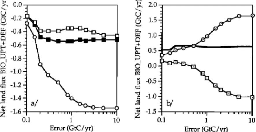
ñ0.5 Gt C yr• for tropical ones, with the a priori flux magnitude for BIO_UPT being set to zero. Therefore, in the extreme case when initial errors tend to zero, the inferred biospheric fluxes also tend to zero over nontropical land areas. Figure 1 plots the inferred net biospheric flux as a function of initial errors (5;) in the Northern Hemisphere and in the tropics. When the initial error value is increased from 0 to 10, the inferred fluxes are able to change and may relax toward an asymptotic value. The more rapidly the asymptotic value is reached, the stronger is the constraint imposed by the atmospheric network.In the Northern Hemisphere, we observe two different behaviors (Figure la). The optimized fluxes over North America and Europe are stable within ñ0.1Gt C yr I for 5; > •;0.4 Gt C yr•,
Table 1. Net Fluxes for 14 Sensitivity Tests From S l to Sl4
So SI * S: * S• * S4 S• S• Arctic 0,2 0,1 0,2 0,2 -0,4 North America -0,5 -0,6 -0,8 -0,8 -1,0 Europe -0,3 -0,5 -0,5 -0,6 -1,5 North Asia -1,5 -1,5 -1,5 -1,5 -0,4 South of 30øN 1,0 0,5 0,4 0,3 0,9 Total -1,2 -2,0 -2,2 -2,4 -2,4 North pacific -0,3 -0,2 -0,1 -0,1 0,2 North Atlantic -0,8 -0,8 -0,8 -0,7 -0,1 15øN-15øS 0,6 0,5 0,6 0,6 0,4 15øS-90øS -1,0 -1,0 -1,0 -1,0 -0,8 Total -1,5 -1,5 -1,3 -1,2 -0,2 S7 S8 59 Slo SI1 S12 S13 S14 Land Upta• 0,1 0,0 0,2 -0,3 0,3 0,2 0,1 0,1 0,1 -1,0 -0,4 -0,3 -1,1 -0,5 -0,4 -0,5 -0,5 -1,0 -0,8 -0,2 -0,3 -0,7 -0,2 -0,4 -0,1 -0,3 -0,3 -0,3 -0,8 -1,3 -1,7 -1,0 -0,9 -1,6 -1,5 -1,3 -1,4 -0,5 1,1 1,4 0,6 0,3 0,9 0,2 1,0 0,9 0,3 0,2 -1,2 -1,0 -1,2 -2,1 -1,3 -1,5 -1,0 -1,1 -1,4 -1,4 &eanUpta• -0,3 -0,1 -0,5 0,0 -0,1 -0,3 -0,2 -0,2 -0,3 - -0,7 -0,8 -0,8 -0,5 -0,7 -0,8 -0,7 -0,7 -0,5 -0,8 0,6 0,5 0,6 0,6 0,3 0,6 0,0 0,2 0,6 0,5 -1,1 -1,4 -0,9 -0,7 -1,0 -0,9 -1,0 -0,9 -0,9 -0,8 -1,6 -1,8 -1,6 -0,7 -1,5 -1,4 -1,8 -1,7 -1,1 -1,1
In Gt C yr
1 . SO
is the control
run
from
B99.
SI, S
2 and
S
3 represent
inversions
performed
using
•13C
measurements
as
additional constraints. In S4 we use TM3 transport model instead of TM2. In S 5, no explicit land uptake pattern is considered. In S6, the ocean scenario of Aurnont [ 1998] is used instead of that of Takahashi et al. [ 1997]. Continental influenced monitoring sites have been removed in S 7 (TM2) and S 8 (TM3). InS 9, Pacific cruise data (P01 to P16) have been removed for the inversion. In S! 0 China Sea cruise data have been removed for the inverse calculation. In S 14, Arctic region has been agragated with North
American one, north Asian with European, and North Pacific with North Atlantic. *Performed for 1990-1995 period only.
BOUSQUET ET AL.: SENSITIVITY STUDY OF INVERSE MODELING OF CO2 26,181 ½ -0.2 m -0.4 + -0.6
D• -0.8
¸ • -1.0 • -1.2 • -1.4 • -1.6 2: + • 0.5 o.o • -0.•• -1.0
0.1 ! , ! ! ! , ii I , i , , ! ,11 Error (GtC/yr) 0.1 1 10 Error (GtC/yr)Figure 1. (a) Nontropical and (b) tropical net land flux at continental scale (BIO_UPT+DEF). For North America (solid squares), Europe (open squares) and north Asia (open circles) in Figure 1 a and for tropical America (dotted squares), tropical Africa, and tropical Asia (dotted circles) and the sum of the two previous curves (solid line) in Figure lb.
meaning that for Z above ñ0.4Gt C yr 1, the inferred flux is not altered by the initial guess. In contrast, the inferred flux over northern Asia depends on the first guess estimate for
Z <ñ1.1 Gt Cyrl. This latter flux therefore
requires larger
a priori errors to relax to its asymptotic value, probably because it is less constrained by atmospheric observations than the other two. The arbitrary choice of ñ 1.5 Gt C yr 1 for the initial errors onthis region
in the control
run S O is thus
relevant
considering
the
fact that we want to limit the influence of initial conditions for
regions
where fluxes are highly uncertain.
Including in the
inversion some recent atmospheric measurements over Siberia [Sugawara et al., 1997] could reduce the uncertainties on theinferred
fluxes
over that domain.
It is worth noting
that uptake
over North America does not correlate with uptake over Siberia when the value of Z is increased (Figure 1 a), suggesting that the present set of atmospheric observations is sufficient to separateboth areas, with North America (and Europe) being better
determined than northern Asia.In the tropics
the inferred
flux over South
America
strongly
anticorrelates with the one over Africa and Asia, when the valueof Z increases
(Figure
lb). Over both
regions
an asymptotic
value
is not approached until Z > ñ3.0 Gt C yr 1. Yet, the sum of alltropical
land fluxes is rather constant
within ñ0.1Gt C yrl for
Z > ñ0.5 Gt C yrl. This reveals the poor level of constraintfluxes at a continental
scale
in the tropics,
where only a zonal
average
estimate
can be safely
inferred.
Thus in run So, setting
the value of Z to ñ0.5 Gt C yr I in the tropics
is appropriate
to
produce an unbiased zonal land flux estimate, but the longitudinal partitioning of tropical land fluxes shall not be discussed.2.3. Influence of the a Priori Flux Scenario Patterns
Our choice to optimize net CO 2 fluxes over large continental and ocean regions assumes that spatial patterns are fixed in the a priori fluxes within each region. In order to test the influence of the a priori flux scenario on the result of the inversion, we have
performed
three
sensitivity
studies
where
we modified
the spatial
patterns or the spatial discretisation of initial fluxes.
2.3.1. Spatial discretization
(number of source
regions).
In
order to test the influence of source regions in the inversion we have performed five different model inversions based on a decreasing number of source regions used to optimize the surfacefluxes.
The maximum
number
of source
regions
is 34 (66 source
base functions), corresponding to 16 land fluxes (48 source base functions, see B99), 14 ocean sources, three deforestation sources and one fossil source (Table 2). We decrease progressively the number of source regions down to nine regions (14 source base functions) consisting of three land fluxes (nine source base functions), three ocean fluxes, one deforestation source, and one fossil source (Table 2). All these inversions (Sll to Sl4) are referred to XXbio_YYoce with XX standing for the number of source regions representing land fluxes and YY standing for the number of source regions representing ocean fluxes. In that case, the name of "1 l bio_8oce" corresponds to the control inversion So. One may anticipate that a larger number of source regions allow for more degrees of freedom and relax the effect of
observational constraints.
When the number of source regions decreases from Sll to S14, the ocean uptake decreases from 1.8 to 1.1 Gt C yrl, while conversely, the land uptake increases from 1.0 to 1.4 Gt C yr 1 (Table 3). This trade-off between ocean and land absorption is not entirely symmetric because fossil fuel emissions are also reduced, which explains why the total BIO_UPT + OCE is not constant in Table 3. We verify in this test that an increasing number of regions correlate with a smaller reduction in the uncertainty estimates of the inferred fluxes. This effect can be explained because increasing the number of source regions means reducing the constraint imposed by atmospheric measurements.
Table 2. Description of the Space Discretization of the Inversions Used for the Sensitivity Test
16bio 14oce 13bio 1 loce 1 lbio 8oce 6bio 5oce 3bio 3oce
GPP, RES, BIO UPT OCE DEF FOS Total
48 14 3 1 66 39 11 3 1 54
33 8 3 1 45
18 5 3 1 27
9 3 1 1 14
Number of source base functions for the inverse procedure. "Bio" stands for land fluxes and "oce" stands for ocean fluxes. Each inversion is referred as XXbio YYoce where XX is the number of regions for land
fluxes (it has to be multiplied by 3 to have the number oœ source base
26,182
BOUSQUET
ET AL.: SENSITIVITY
STUDY
OF INVERSE
MODELING
OF CO
2
Table 3. Net Fluxes and Errors for Five Configurations of the Inversion Using Decreasing Number of Source Base Functions
Sll S12 S13 SO S14
16bio 14oce 13bio 1 loce 1 lbio 8oce 6bio 5oce 3bio 3oce
Land uptake Arctic 0,1 q- 0,3 0,1 q- 0,3 0,2 q- 0,3 0,1 q- 0,2 - - - North America -0,5 q- 0,5 -0,5 q- 0,5 -0,5 q- 0,6 -1,0 q- 0,4 -0,8 -+ 0,4 Europe -0,3 q- 0,9 -0,3 q- 0,9 -0,3 q- 0,8 -0,3 q- 0,6 -0,8 -+ 0,4 North Asia -1,3 q- 0,7 -1,4 q- 0,7 -1,5 q- 0,7 -0,5 q- 0,4 - - - South of 30øN 1,0 q- 1,3 0,9 q- 1,2 1,0 q- 1,0 0,3 q- 0,9 0,2 + 0,6 Total -1,0 q- 1,8 -1,1 q- 1,8 -1,1 q- 1,6 -1,4 q- 1,2 -1,4 + 0,8 Ocean uptake North Pacific -0,2 q- 0,3 -0,2 q- 0,3 -0,3 q- 0,2 -0,3 q- 0,2 -0,8 -+ 0,3 North Atlantic -0,7 q- 0,3 -0,7 q- 0,3 -0,8 q- 0,3 -0,5 q- 0,3 - - - 15øS-15øN 0,0 q- 0,4 0,2 q- 0,3 0,6 q- 0,2 0,6 q- 0,1 0,5 + 0,1 90øS-15øS -1,0 q- 0,4 -0,9 q- 0,4 -1,0 q- 0,3 -0,9 q- 0,3 -0,8 + 0,2 Total -1,8 q- 0,7 -1,7 q- 0,7 -1,5 ñ 0,5 -1,1 q- 0,4 -1,1 + 0,4
In Gt C yr 1 . "Bio"
stands
for net
land
uptake
(BIO_UPT+DEF)
and
"oce"
stands
for ocan
uptake.
The
sum
of BIO_UPT
and
OCE
is not
constat
because fossil fuel emissions are modified.The results of the three inversions 16bio_14oce, 13bio_l loce, and 11 bio_8oce differ markedly one from another in the tropics (Table 3). The ocean equatorial source even drops to zero in run 16bio_l 4oce, which has four distinct ocean regions in the tropics. This is rather unrealistic regarding direct estimates of the fluxes [Andrie et al., 1986' Boutin and Etcheto, 1997; Metzl et al., 1995].
When the number of regions is increased jointly with a reduction of the tropical sea-to-air flux, a stronger land source is inferred so that the sum of all tropical fluxes is conserved within 0.4 GtC yr 1. This suggests that tropical fluxes are poorly constrained not only over land regions but also over some ocean regions, including those containing a measurement site (GMI, ASC, SEY, Pacific Ocean cruises). The atmospheric circulation in the tropics generates a couplet between rather weak horizontal zonal winds and strong vertical motion in the rising branch of the Hadley cells [Heimann and Keeling, 1989], which may qualitatively explain why a tropical sea level station has less spatial representativeness than a midlatitude one.
When the number of regions is reduced compared to So settings, in runs 6bio_5oce and 3bio_3oce, a correlation appears between the flux estimates of North America and Eurasia. The North American sink is 2 times larger than in S O and the Eurasian uptake is abated accordingly. This solution is more in agreement with Fan et a/'s [1998] results even if North America remains smaller than in their study. In the 3bio_3oce case the inferred solution is nudged by the small number of degrees of freedom. The solution for the average Northern Hemisphere land uptake differs significantly between runs 6bio 5oce and 3bio 3oce compared to So but remains stable if the number of regions becomes larger than in So.
Overall, using too many degrees of freedom leads to having numerous flux estimates that give a good fit at monitoring sites, whereas using too few degrees of freedom tends to nudge the solution and provides a poor fit to the observations. In both cases the validity of the inferred solution is doubtful, especially for poorly constrained regions. The possibility of using many more
degrees of freedom using an adjoint model approach is still under investigation [Kaminski et al., 1997]. The choice of 1 lbio_8oce as the reference inversion appears as a good compromise
between these two limitations.
2.3.2. Land spatial patterns of the prior sources within each region. In the sensitivity run S5, we test an alternative solution to represent land uptake (BIO_UPT) within each region used for inverse calculation. This is obtained by adjusting the sum of gross primary production (GPP) and total respiration (RES) over each region. In other words, we do not use the explicit land uptake component (BIO_UPT) as in our control inversion So. The sums of RES and GPP for each region are set to zero in the prior estimate and are associated with error bars equal to those assigned to BIO_UPT in So. The results are listed in Table 1. At the global scale the fluxes inferred for Ss are similar to those obtained in So within 0.2 Gt C yr I . However, the North American sink is increased by a factor of 2 in Ss compared to So and reaches up to 1.0+0.6 Gt C yr 1 . Concomitantly, the Eurasian sink decreases by 0.3 Gt C yr-, and the terrestrial source in the tropics increases by 0.2 Gt C yrl. We conclude from this that important modifications in the optimized sources and sinks can occur at a continental scale in response to changing the prior spatial regional patterns of land uptake. We further investigated the case of North America to determine which region (temperate / boreal) is responsible for a more pronounced uptake in S, compared to So. In &, the flux apportionment between boreal and temperate America is of +0.4Gt C yrl in the boreal zone (source) against-1.4 Gt C yr • in the temperate region (sink). In contrast, So produces a more even distribution of the sink, with boreal North America being a small source of 0.1 Gt C yr I and temperate North America being a sink of 0.6 Gt C yr•. The overall increase in the North American sink between So and S s is a direct effect of changes in prior spatial patterns: in So we use the Friedlingstein et al. [1995] flux pattern that has proportionally more flux and spatial structures in the boreal ecosystems (compared to temperate or tropical ones) than GPP or RES have. Changes in the boreal versus temperate partition
BOUSQUET ET AL.: SENSITIVITY STUDY OF INVERSE MODELING OF CO2 26,183
suggests that these two regions are not well constrained separately in the inverse procedure. In fact, only two stations (KEY and SBL) are located close and downwind of the eastern coast of North America, other sites being either continental (NWR, UTA) or situated on the west North American coast (CMO, OPW, CSJ).
2.3.3. Ocean spatial patterns of the prior sources within each region. In this section we perform an inversion S 6 that differs from So by the use of an alternative air-to-sea CO2 flux field. The test inversion S6 uses as a priori the monthly global sea-to-air fluxes distribution calculated by Aumont [ 1998] from the three dimensional (3-D) ocean carbon model (Institut Pierre Simon Laplace, IPSL) based on general ocean circulation model OPA7-NPZD [Delecluse et al., 1993; Six and Maier-Reimer,
1996] The results of that inversion (S6) indicate a marked increase of the global ocean sink, on the order of 0.4 Gt C yrl compared to S o , whereas the global land uptake is abated by the same amount (Table 1). The change between So and S6 is caused primarily by an increase in the Southern Ocean CO2 uptake from 1.0 to 1.4 Gt C yr I . This is attributed to the existence of different spatial patterns in the two sets of prior air-to-sea fluxes from Takahashi et al. [1997] and Aumont [1998] over the southern ocean. Takahashi et al., [1997] do not have strong longitudinal gradients in the sea-to-air fluxes, since the ApCO2 measurements that they have used are rather scarce south of 40øS to constrain their extrapolation method. In the model study of Aumont, [1998], limited areas of strong outgassing occur within the band 40øS -60øS and create a complex longitudinal structure, possibly as an artifact of the ocean model simulation (O. Aumont, personal communication, 1997).
The existence of such localized source areas, sometimes close
to measurement sites, can partly offset the uptake of CO 2 by subtropical and sub-Antarctic surface waters that is inferred from the existing monitoring sites and can force the inverse procedure to infer a larger sink in the whole latitude band in order to match the atmospheric observations. One of these sources is located in
the sub-Antarctic Indian Ocean and therefore influences the
Amsterdam Island site (AMS), Cape Grim (CGO), and Baring Head station (BHD). Table 1 also shows that tropical regions are
a net source
to the atmosphere
of 1.4 Gt C yrl (+0.4 Gt C yr -1
compared to So), while the Northern Hemisphere land uptake shifts from 2.1 Gt C yr I in So to 2.4 Gt C yr • in S6. Thus the meridional distribution of the terrestrial carbon uptake is adjusted (decrease in the tropics and increase in the north) in order to compensate for the ocean effect noticed above (increase in the south and small decrease in the north).2.3.4. Discussion. For both changes in land and ocean uptake spatial patterns, one can notice that the smaller the spatial scale is, the more significant the changes are. At global and hemispheric scales the inverse problem is constrained enough to almost give the same inferred fluxes with all the patterns we have tested. However, at regional or continental scales, differences reach 0.5 Gt C yr • (a factor of 2 for North America sink) but remain compatible with error bars of So. Concerning space discretization of fluxes, it appears that it is difficult to increase the number of regions in the tropics without modifying significantly the CO 2 budget at continental scale.
With these tests we see that spatial patterns of initial sources become important at the scale used to make the spatial discretization and the inverse calculation. So, as mentioned by Peylin et al. [ 1999] it may be important to discuss inferred fluxes at a spatial scale larger than the calculation scale. As atmospheric network density increases, one can attempt to adjust more closely
the space discretization in order to limit its influence on inferred fluxes while keeping a good state of constraint. A coherence has to be found between atmospheric constraint, model resolution, and space and time discretization of fluxes. However, if one wants to increase the number of regions (over the continents of the Northern Hemisphere, for instance) by a large factor, the computing cost of the response functions becomes a problem. One possible solution to this issue is to use an adjoint model to calculate source base function for all pixels of the transport model and make a posteriori spatial rearrangements [Kaminski et al., 1997].
Another important point is the time discretization of fluxes. In our approach, we run monthly flux fields in the transport model, but we only optimize annual fluxes (against monthly averaged observations) in the inverse procedure. As most atmospheric data are provided on a weekly or a monthly base, the method could be adapted to optimize monthly fluxes. This would increase the degrees of freedom by a factor of 12. The study of the influence of time discretisation on optimized fluxes in an important issue [Peylin et al., 1999].
3. Influence of Atmospheric Transport
As recently shown, one main source of uncertainties in the results of atmospheric CO2 inversions appears to be the modeled atmospheric transport [Law et al., 1996; Denning et al., 1997]. Inversion S4 (Table 1) is performed with the same characteristics as S o but uses the TM3 transport model [Heimann, 1995] instead of TM2. The TM3 model is based on the same wind fields as
TM2 but has finer vertical (19 sigma levels instead of 9) and horizontal (4 ø x 5 ø instead of 7.5 ø x 7.5 ø) resolution. The same source base functions as in inversion S o are run in model TM3, and the outputs are used in the standard inverse procedure. The flux solution of S 4 exhibits major differences from So. The net
land uptake
of CO 2 is multiplied
by a factor
of 2 (2.4 Gt C yr l)
whereas the ocean uptake drops down to 0.2 Gt C yr • . Over the continents, the sink in North America increases from 0.5+0.6 up to 1.0-J=0.4 Gt C yr•. The European sink is multiplied by a factor of 5 (1.5+0.5 Gt C yrl), whereas the sink over northern Asia is reduced from 1.5+0.7 to 0.4+0.4 Gt C yrl.Such large differences between the results of So and S4 are mainly due to the rectifier effect of atmospheric concentrations that is present in the TM3 model (see B99, section 2). This effect contributes to the increase of the annual mean modeled CO2 concentration over the Northern Hemisphere continents with respect to the marine boundary layer concentrations. This is especially true at European "continental" sites such as BAL, SCH, WES, or TAP. The continent-to-ocean CO 2 concentration gradients predicted by TM3 are larger than the one for TM2 or for the observations. As a consequence, the inferred sink over Northern Hemisphere continents is much larger for the modeled concentrations to match the observed ones. This is especially true over Europe where more continental sites can be found. Another consequence of the TM3 rectifier is that the global ocean uptake drops to 0.2 Gt C yr• in order for the sum of global land plus ocean fluxes to match atmospheric trend. As a result, the Northern Hemisphere oceans are no longer a significant net sink in S4, as compared to So. This result is doubtful as the North Atlantic has been determined to be a significant net sink [Lef•vre, 1995; Takahashi et al., 1997]. Finally, it is interesting to observe
that the differences between TM3 and TM2 almost vanish in the tropics. The continental fluxes south of 30øN and the ocean
26,184 BOUSQUET ET AL.: SENSITIVITY STUDY OF INVERSE MODELING OF CO 2
fluxes south of 15øN are changed by < 0.2 Gt C yr 1 in S4 as compared to So.
The partitionning of the Northern Hemisphere carbon flux over land seems to be overestimated in TM3, which may reflect a
model overestimate of the continental concentrations because of
the "rectifier" effect. In this context there is a problem of
coherence between the treatment of continental sites in the TM3
model (no selection of continental data according to wind speed and direction or any other criterion) and the subsampling of CO2
data at continental stations that are most of the time selected to
remove some the local sources influence. According to Ramonet and Monfray [ 1996] a model presenting a higher horizontal and vertical resolution is more sensitive to subscale processes such as local meteorological effects or regional environmental effects (presence of a forest, of factories, etc.). The TM3 model has a
better horizontal and vertical resolution than TM2 and should
therefore provide a more realistic representation of the atmospheric transport than TM2. To improve the coherence between model and selected data, we have to improve the representation of continental sites in the model and to test vertical subgrid scale mixing parametrizations (convection and diffusion).
4. Influence of Atmospheric Measurements
4.1. Influence of CO2 Atmospheric Network
4.1.1. Individual site influence. The first test we have
performed is a bootstrap test. The principle is to remove each site one by one from the station list and to compare the results of all
the inversions calculated with 76 sites instead of 77 to the
standard inversion So. For each region we compute the difference of inferred net flux between the inversion performed without station XXX and So. We keep differences when they are greater than 0.1 Gt C yr 1 for one given region. Only three stations induce differences larger than 0.1 Gt C yr I .
First, removing Baltic station (BAL) changes deeply the partition of the Northern Hemisphere land uptake: Europe becomes a sink of 1.1 Gt C yrl (0.3 in So) while the sink over north Asia is reduced to 0.8 Gt C yrl (1.5 in So). The sink over North America in only reduced by 0.1 Gt C yr I . This impressive result is probably due to a bad representation of BAL station by a
model like TM2 that has a coarse horizontal resolution. BAL
flasks are taken over the Baltic Sea whose extension in longitude in of the order of magnitude of one grid box of TM2. BAL is very high in CO2 in the data on annual average (see B99, Figure 4). Thus, if we do not use it, the inverse calculation increases the sink over Europe that was limited by the presence of BAL. Consequently, the sinks over north Asia and North
America are reduced. One can notice that the North American
sink is much less reduced than the north Asiatic sink. Actually, the total Eurasian land uptake is only modified by 0.2 Gt C yr• by this test.
Then, removing the UUM Mongolian station induces an increase of 0.2 Gt C yrl for the north Asiatic land uptake (-1.7 instead of- 1.5). UUM is a site located high above sea level and is also probably not well represented by the model. Finally, removing Sable Island station (SBL) increases the North American sink by 0.2 Gt C yr 1 (-0.7 instead of-0.5). SBL is a bit high in CO2 compared to what the model predicts. If we do not use it the inverse procedure has a tendency to increase the north American sink. In conclusion, except for B AL site, other stations have a small individual impact on the results of our control inversion So.
4.1.2. Continental sites. The present CO 2 atmospheric
network is the most important network for trace gas measurements. However, its density is highly variable geographically. Some regions have many monitoring sites (Europe, for instance) and some other regions have no sites at all (South America and Siberia, for instance). Most of the sites are marine boundary layer sites. However, 10 sites located inland or under land influence have been added to our control inversion So. As a sensivity test, we have removed these 10 sites from the inverse calculation (BAL, WES, SCH, CIM, NWR, UTA, RYO, TAP, QPC, KSN). This test is performed for both TM2 (S7) and TM3 (S8) models.
For TM2, net land uptake and net ocean uptake are almost unchanged compared to So (+0.2 Gt C yrl). Note, however, that in this test the fraction of the biospheric sink located in the mid and high latitudes of the Northern Hemisphere is reduced by 15% and drops to 1.8GtCyrl (2.1GtCyr 1 in S0). In contrast, important changes occur for TM3 model. Removing sites under continental influence leads to increase the global ocean uptake by
0.5 Gt C yrl and to decrease
the land uptake
by 0.4 Gt C yr -1.
The Northern Hemisphere land uptake is reduced by 30% compared to the standard TM3 inversion (S4). The decrease of the land uptake over 15øN in both TM2 and TM3 can be explained by the reduction of continent to ocean gradients caused by the exclusion of continental sites in S 7 and S8. The decrease is twice as important in TM3 than in TM2 because the continent to ocean contrasts of a priori modeled atmospheric concentrations are much larger in TM3 due to a stronger rectifier effect.
One can also notice a significant balance of net land uptake between north Asia and Europe for both models. In the TM2 inversion (S7), the north Asia sink is reduced to 1.0 Gt C yr 1 and the European sink is increased to 0.7 Gt C yr 1. This effect is coherent with the individual influence of BAL station noticed above. In the TM3 inversion (S8), the north Asia sink is increased up to 0.9 Gt Cyrl and the European sink is reduced to 0.2 Gt C yr I . It is interesting to note that if both models agree on the amplitude of the uptake over Siberia, there is no agreement between the amplitude of European and North America land uptakes. The sink is located preferentially over North America
for TM3 and over north Asia for TM2.
Using mainly marine boundary layer sites in inversions S7 and S 8 should remove most of the influence of the rectifier effect that is present in TM3. However, the two models still fail to converge to the same partition of fluxes for the Northern Hemisphere. This means that atmospheric transport is a major source of uncertainties in inverse studies at all spatial scales. Moreover, as long as there is no precise quantification of the rectifier effect above continents, there is no way to reduce the uncertainty due to transport models. The quantification of the rectifier effect remains an open and major question that will have to be addressed in the near future if one wants to use transport models for atmospheric inversions. The third phase of the TRANSCOM experiment should go in this direction (TRANSCOM is an international model intercomparison experiment that has been running since 1994; see Law et al. [1996] and Denning et al. [1997]).
4.1.3. Cruise data influence. In So we use two sets of atmospheric data built from marine cruises in the Pacific Ocean (P01 to P 16) and in the China sea (CO 1 to C07). In order to see the influence of these data that have been aggregated per latitude band, two inversions are performed without them.
In S9, Pacific cruise data are removed from the inverse calculation. One can see on Table 1 that changes concerning net
BOUSQUET
ET AL.: SENSITIVITY
STUDY OF INVERSE
MODELING
OF CO2
26,185Nevertheless, ocean uptake is modified at the hemispheric scale. The contrast between Northern Hemisphere ocean sink and equatorial source is reduced by 0.6 Gt C yrl when compared to
So: Equatorial
source is reduced
by 0.3 Gt C yrl whereas
Northern Hemisphere sink is also reduced by 0.3 Gt C yr•. In the tropics, Pacific cruise data present higher CO2 concentrations than other stations of the same latitude band (+0.2 to + 1.2 ppm). North of 15øN, the situation is the opposite with Pacific cruises presenting lower CO2 concentrations than other stations of the same latitude band. Removing Pacific cruises from the inverse calculation thus implies that a smaller tropical source and a smaller midlatitude sink are needed to match the observations.In S•0, South China Sea cruises have been removed from inverse calculation (C01 to C07). In our control inversion So,
tropical
Asia is found to be a source
of 0.84-0.4
Gt C yr•. This
estimate drops to 0.24-0.4 Gt C yr 1 in test S10 (Table 1). China Sea data which have been aggregated into seven stations that are close to China and Southeast Asia exhibit CO2 concentrations 0.5 to 2.0 ppm higher on average than other stations at the same latitude over the central Pacific Ocean. As a consequence, the inverse procedure places a substantial source over tropical Asia between 10øS and 30øN to fit these stations. This source is reduced by 60% without these sites. The Northern Hemisphere land uptake is also reduced by 15%. Note, however, that north Asia land uptake is unchanged in S•0 when compared to So. 4.1.4. Japanese flight data influence. Vertical profiles of CO2 have been already used to test the vertical transport in atmospheric models [Monfray et al., 1996]. As most of CO2 fluxes are exchanged at the surface, aircraft measurements can give an integrated view of the exchange of carbon. It is interesting to quantify the influence of these data on the results of the inversion. To do so, we have performed an inversion without data from the Japanese vertical profile. No significant changes in net fluxes were noted at global and continental scales (test not reported in Table 1). However, within north Asia we note a balance of the net land uptake between boreal Asia and temperateAsia. In So, boreal
Asia has a sink of 0.6 Gt C yr• and temperate
Asia has a sink of 0.9 Gt C yrl, whereas without the Japanese profiles the partition is the opposite. This test shows that the Japanese vertical profile is important to constraining the partition of land uptake at a regional scale within the Asian continent. 4.1.5. Calibration issue. In inversion S O , data from different atmospheric network are aggregated together to increase the constraints on the surface fluxes. The intercalibration problem between these networks is still not completely resolved even if a lot of work has already been done by flask exchange campaigns between laboratories involved in atmospheric CO2 measure- ments. Tanks containing calibration gas are exchanged between more than 10 groups (every 4 years). Our group is also involved in a flask exchange program with Division of Atmospheric Research (CSIRO/DAR, Australia) and National Oceanographic and Atmospheric Administration Climate Monitoring and Diagnostic Laboratory (NOAA/CMDL, United States Of America) at the Cape Grim station (CGO). However, some measurement groups are still not involved in such exchange programs. This limits the use of their stations in inverse procedures.We perform an inversion where annual means of all data from NOAA CMDL network are increased by 0.25 ppmv (test not reported in Table 1). This value is in the range of intercalibration problem as suggested by NOAA CMDL group (K.A. Masarie, personal communication, 1998). The results of the inverse procedure are modified by < 0.1 Gt C yr• at continental scale.
However, the global offset for CO2 concentrations taht we optimize in the inverse procedure is increased by 0.2 ppmv compared to So offset. This change can be explained by the fact that NOAA CMDL network represents the largest network (80%). Thus the inverse procedure preferentially modifies the offset instead of the regional fluxes.
We have performed two other sensitivity tests in which we increase by 0.5 ppmv the concentrations of the stations either of the IPSL Laboratoire des Sciences du Climat et de
l'Environnement (MHT, AMS) or of the CSIRO DAR (CGO, CG4, CG6, BHD, MAQ, MAW). For the IPSL LSCE network the main change is a limited decrease of 0.2 Gt C yri of the sub-Antarctic subtropical sink. For the CSIRO DAR, the main differences with So is a small increase of the southern nontropical land net source of 0.2 Gt C yri and a small decrease of the equatorial ocean source of 0.1 Gt C yri. Effects for other regions remain under 0.1Gt C yrl.
4.2. Influence of 1513C Measurements
4.2.1. Methodology. The control inversion S O is performed
without
using
1513C
measurements.
In this
section
the influence
of
adding
1513C
measurements
as an additional
constraint
to regional
fluxes is studied. Methodology and specific formalism to include 13C measurements as additional constraints on net CO2 sourcesand sinks
is described
in the appendix.
Roughly,
1513C
can be
expressed as a combination of the modeled responses of CO2 source base functions and of the modeled responses of source base functions for the CO2 gross fluxes (corresponding to disequilibrium terms). Each coefficient of this combination is the product (hereinafter called isoflux) of a CO2 source strength and of an isotopic signature. Isoflux is linearized according to Tarantola [ 1987] and Hein et al. [ 1997] formulations. Thus, for1513C
we not only optimize
net CO2 annual
flux strengths
but also
one isotopic signature per source.
We use 1513C measurements from 24 monitoring sites that have been progressively available since 1990 as part of the NOAA/CMDL air sampling program [Trolier et al., 1996]. The reference period for this test is 1990-1995 to insure consistency
between
CO2 and
•13C data.
Over
that
period
the global
CO2
rate
of increase
is 1.34-0.1
ppm
yr -• and
the global
1513C
trend
is set
to
-0.025%oyr
-•. The fossil source strength is assigned to
6.24-0.3 Gt C yr• Three different inversions are presented toexamine
the specific
role
of 15
•3C
measurements:
S• has
the same
constraints as So (i.e., CO2 measurements only) but covers theperiod
1990-1995,
S2
is identical
to S• but
includes
the
15•3C
data
and trend, and S3 is identical to S2 but the isotopic disequilibria and fluxes signatures are maintained to a fixed value (identical to the priors).
4.2.2. Modeled
•13C. Figure
2 compares
the modeled
•13C
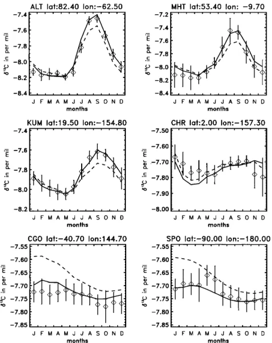
values (a priori and optimized) at six stations of the NOAA CMDL network with the atmospheric observations.Figure
2 shows
that the fit to the monthly
15•3C
observations
is
satisfying overall at all sites but is not as good as the fit obtainedfor CO2 only. As for So, the S1 inversion
that includes
•3C
performs better for nontropical sites. The reasons of the inversion shortcoming in the tropics could be the same as that for CO2 (poor constraint on the continental fluxes from the atmosphericstations)
but could
be also
specific
to 15•3C
(the crudeness
of the
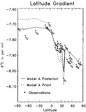
ocean disequilibrium representation or absence of seasonality in the isotopic signatures). Figure 3 presents the simulated north tosouth
annual
1513C
concentrations
at the monitoring
sites. The
26,186 BOUSQUET ET AL.' SENSITIVITY STUDY OF INVERSE MODELING OF CO2
-7.4
-7.6
-8.4
ALT lat:82.40 Ion'-62.50
i i , i i i , , i , , ' i I i I i i i i i i i J FMAM J J A S ON D months -7.2 -7.4
E -7.6
Q' --7.8 .c_ .o -8.0 -8.2 -8.4 MHT laf:55.40 Ion' -9.70 , , , , , , , , , , , ' ' ' ' ' I I I I I I I ' J FMAM J J A S 0 N D months -7.4 = -7.6 E o_ -7.8 .c_ - '• -8.0 -8.2KUM laf:19.50 Ion'-154.80
, , , , , , , , , , , . J F MAM J J A SO N D months -7.50 -7.60 .-7.70 -7.80 -7.90 -8.00 CHR lat'2.00 Ion'-157.3;0 , , , , , , , , , , , i , , i I I I I I I I ' O FMAM O O A S ON D months -7.60 ._
E -7.65
o_ -7.70 .c_ .o -7.75 -7.80 -7.85CGO laf'-40.70 Ion'144.70
-7.55 ... . i i i , i , i i i i ' J FMAM J J A S ON D months -7.55 -7.60 o_ E -7.65 Q' --7.70 ?_ .0 --7.75 --7.80 -7.85
SPO lat:-90.00 Ion'-180.00
, , , , , , , , , , ,
i i , i ,
J FMAM J JASON D months
Figure
2. Modeled
and
observed
•513C
concentrations
for six monitoring
sites
used
in inversion
S1.
Dots
stand
for
atmospheric
data (one climatological
year of observations
averaged
over the 1990-1995
period).
Dashed
line is for
the a priori modeled concentrations Solid line is for the optimized model concentrations.813C
profile,
which
indicates
a terrestrial
uptake
and matches
rather closely the observed values at most of the sites. 4.2.3. Inferred fluxes. Table 4 presents the optimized net CO2
fluxes and errors
obtained
respectively
in S•, S2, and S3 at the
global and continental scale. Table 4 is a detailed version of
Table 1 for inversions
Sl, S2, and S
3. The results
of S• (only CO 2
data) differ slightly from those of So and show an increase of the Northern Hemisphere land uptake from 2.1 to 2.5 Gt C yr• Conversely, the continental tropical source is reduced from 1.0 to 0.5 Gt C yrl. Such values are consistent with studies that have estimated a larger biospheric sink during the early 1990s than in the 1980s [Ciais et al., 1995b; Francey et al., 1995; Keeling etal., 1996] . Comparing
the results
of S2 and S1, one can clearly
see
that
using
813C
measurements
does
not
induce
major
changes
in the inferred net CO2 fluxes. Resulting differences do notexceed
+0.1Gt C yrl at a continental
scale. Only, a slight
reduction of errors, of the order of +0.1Gt C yr 1 , is achieved over
the Northern
Hemisphere
land areas
when
the 813C
constraint
is
included. This result, which is surprising considering the
importance
of 813C
measurements
in previous
studies
[Ciais
et
al., 1995b; Enting et al., 1995], can be attributed to four main
causes.
First, we only use 24 stations
for 813C,
versus
80 for CO2.
This difference
clearly
gives
a lower
weight
of the 8•3C data
in
the inverse
procedure.
Second,
uncertainties
on the monthly
813C
values constructed from the flask measurements are comparatively larger than for CO2 (synoptic variability, analytical precision, and interannual variability). Third, we include some stations under strong continental influence in the inversion procedure (e.g., BAL, TAP, WES, or SCH). Thus CO 2 gradients between oceans (marine boundary layer sites) and continents are already a powerful constraint on the geographicalBOUSQUET ET AL.' SENSITIVITY STUDY OF INVERSE MODELING OF CO2 26,187 -7.60 -7.7O -7.80 -7.90 -8.00 -8.10
Latitude
Gradient
Model A PosterJori
---Model A Priori
Observations -90 -60 -50 0 50 60 90 LatitudeFigure 3. Modeled
and observed
•13C north to south
annual
concentrations for six of the 24 monitoring sites used in inversion S1. Dots stand for atmospheric data (one climatological year of observations averaged over the 1990-1995 period). Dashed line is for the a priori modeled concentrations Solid line is for the optimized model concentrations.
partitioning of the fluxes. In this context, S• yields a set of continental and ocean fluxes which is fully compatible with the
b•3C
information,
in such
a manner
that
adding
15•3C
in S2 does
not changes the inferred sources magnitude. Finally, one mustconsider
that the inverse
procedure
based
on 15•3C
optimizes
the
net fluxes, as well as the gross fluxes (via the disequilibria) and the isotopic signatures. This means that there could be a "temptation" for the inverse procedure to change the disequilibriaor the isotopic
signatures
to match
the 15•3C
constraint
because
these
parameters
are only constrained
by the 1513C
observations
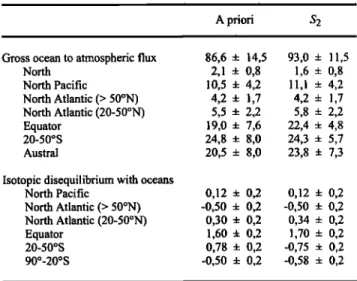
and not by the CO2 measurements. The changes inferred in the ocean disequilibrium are the only significant ones among all theparameters
that are "determined"
by 15•3C.
Biospheric
disequilibrium is not significantly modified as it is linked to total respiration which is already constrained by CO2 measurements. Table 5 shows the a posteriori and a priori disequilibrium fluxes with the ocean for S• and S 2. It indicates that the inverse procedure preferentially modifies the isotopic disequilibrium
values
to fit the •13C data
and
especially
the 15•3C
trend,
which
is
a strong constraint on the inversion. In order to test this last hypothesis, we have performed an inversion S3 where we maintained all disequilibrium fluxes and isotopic signatures to their initial values by prescribing a very small error. In that case, the changes in the CO2 net fluxes are significantly more important in S3 than in S2 ß For example, global land uptake
increases
by 0.4 Gt C yr
-1 in S3 and
only
by 0.1 Gt C yr
-• in S2 ß
In S3 the inversion procedure can only adjust the CO2 net
exchange
to fit (•13C
data
which
enhances
the influence
of (•13C
on the solution.5. Summary and Discussion
In order to summarize the differences between each inversion and our control inversion So, we have calculated the Z m coefficient as the mean absolute difference between fluxes
inferred in Sn (n represents the different tests) and fluxes inferred in So for the nine regions defined in Table 1 (see Figure 4). Zm are sorted and presented in a decreasing order. Figure 4 also plots the mean value of the a posteriori uncertainties at continental and ocean basin scale for all inversions which is +0.4 Gt C yr 1. One can notice that all Zm remain below the mean a posteriori uncertainty except for run S4, which corresponds to the use of the TM3 model. Modeled atmospheric transport is largely the most sensitive component of our study. The second most sensitive component is the influence of the spatial patterns given to the a priori fluxes (S 6 and Ss), especially for land uptake of CO 2. Then another sensible parameter is the use of continental sites that are not well represented in the model (such as BAL station).
The influence of each component depends on the spatial scale that is considered for the analysis. Changing the atmospheric transport model from two extreme behaviors with respect to the rectifier effect (TM2 and TM3) modifies the optimized fluxes and partitions between oceans and continents at all scales, from regional to global. This is a major limitation of current inverse modeling to constrain the regional carbon cycle, as mentioned in
section 3. For all other tests the modifications on the inferred
fluxes remain limited to regional and/or continental scales and remain most of the time within a posteriori uncertainties. Especially, some components such as flux uncertainties or number of source regions are very sensitive for poorly constrained regions like the tropical lands. We also see that the a posteriori fluxes at a continental scale (e.g., tropical America versus tropical Asia) depend critically on the a priori error given to the land fluxes. For poorly constrained regions like tropical
continents, the zonal mean of fluxes is much better constrained
Table 4. Regional Results of the Inversions S1, S2 and S 3
S1 S2 S3
Fossil fuel emissions 6,2 ñ 0,3 6,1 ñ 0,3 6,1 ñ 0,3 Continents -2,0 ñ 1,6 -2,2 ñ 1,5 -2,4 ñ 1,4 Arctic 0,1 4. 0,3 0,2 4. 0,3 0,2 4. 0,3 North America -0,6 4. 0,6 -0,8 4. 0,5 -0,8 4. 0,4 Europe -0,5 4. 0,8 -0,5 4. 0,7 -0,6 4. 0,7 North Asia -1,5 4. 0,7 -1,5 4. 0,6 -1,5 4. 0,6 South of 30øN * 0,5 4. 1,0 0,4 4. 1,0 0,3 4. 1,0 Oceans -1,5 4. 0,4 -1,3 4. 0,5 -1,2 4. 0,4 North Pacific -0,2 4. 0,2 -0,1 4. 0,2 -0,1 4. 0,2 North Atlantic -0,8 4. 0,3 -0,8 4. 0,3 -0,7 4. 0,3 15øN-15øS 0,5 4. 0,1 0,6 4. 0,1 0,6 4. 0,1 90øS-15øS -1,0 4. 0,2 -1,0 4- 0,2 -1,0 4. 0,2
In Gt C yr 1 . S 1 is performed under the same conditions as S O but for
1990-1995
period.
S
2 and
S
3 are
two
sensivity
runs
using
b13C
data
as
an additional constraint.
* Deforestation and biospheric sink have been added in the tropics for both a priori fluxes and a posteriori fluxes. The reference period is 1990-


![[PDF] Cours Pascal les structures itératives pdf | formation informatique](data:image/gif;base64,R0lGODlhAQABAIAAAP///wAAACH5BAEAAAAALAAAAAABAAEAAAICRAEAOw==)