HAL Id: hal-02935080
https://hal.archives-ouvertes.fr/hal-02935080
Submitted on 10 Sep 2020
HAL is a multi-disciplinary open access
archive for the deposit and dissemination of
sci-entific research documents, whether they are
pub-lished or not. The documents may come from
teaching and research institutions in France or
abroad, or from public or private research centers.
L’archive ouverte pluridisciplinaire HAL, est
destinée au dépôt et à la diffusion de documents
scientifiques de niveau recherche, publiés ou non,
émanant des établissements d’enseignement et de
recherche français ou étrangers, des laboratoires
publics ou privés.
A Relaxation-based Approach for Mining Diverse Closed
Patterns
Arnold Hien, Samir Loudni, Noureddine Aribi, Yahia Lebbah, Mohammed
Laghzaoui, Abdelkader Ouali, Albrecht Zimmermann
To cite this version:
Arnold Hien, Samir Loudni, Noureddine Aribi, Yahia Lebbah, Mohammed Laghzaoui, et al.. A
Relaxation-based Approach for Mining Diverse Closed Patterns. European Conference on Machine
Learning and Principles and Practice of Knowledge Discovery in Databases 2020, Sep 2020, Gand,
Belgium. �hal-02935080�
Diverse Closed Patterns
Arnold Hien2, Samir Loudni2,3 , Noureddine Aribi1, Yahia Lebbah1, Mohammed
Laghzaoui1, Abdelkader Ouali2, and Albrecht Zimmermann2
1
University of Oran1, Lab. LITIO, 31000 Oran, Algeria
2
Normandie Univ., UNICAEN, CNRS – UMR GREYC, France
3
TASC (LS2N-CNRS), IMT Atlantique, FR – 44307 Nantes, France
Abstract. In recent years, pattern mining has moved from a slow-moving re-peated three-step process to a much more agile iterative/user-centric mining model. A vital ingredient of this framework is the ability to quickly present a set of di-versepatterns to the user. In this paper, we use constraint programming (well-suited to user-centric mining due to its rich constraint language) to efficiently mine a diverse set of closed patterns. Diversity is controlled through a thresh-old on the Jaccard similarity of pattern occurrences. We show that the Jaccard measure has no monotonicity property, which prevents usual pruning techniques and makes classical pattern mining unworkable. This is why we propose anti-monotonic lower and upper bound relaxations, which allow effective pruning, with an efficient branching rule, boosting the whole search process. We show ex-perimentally that our approach significantly reduces the number of patterns and is very efficient in terms of running times, particularly on dense data sets.
1
Introduction
The original data analysis model based on pattern mining consists of three steps in a kind of multi-waterfall cycle: 1) a user chooses the values of one or several mining parameters, 2) an underlying engine extracts patterns (often taking not inconsiderable time to do so), and 3) the user sifts through a (potentially very large) set of result patterns and interprets them, using their insights to return to the first step and repeat the cycle.
Recently, this approach has been challenged by an increasing focus on user-centered, interactive, and anytime pattern mining [14]. This new paradigm stresses that users should be presented quickly with patterns likely to be interesting to them, and typically affect later iterations of the mining process by giving feedback. A powerful framework for taking a variety of user feedback into account is pattern mining via constraint pro-gramming (CP). Much of the current focus in this domain is on user-centered/interactive mining, particularly the ability to elicit and exploit user feedback [9, 14, 18]. An impor-tant aspect of requesting such feedback is that the user be quickly presented with diverse results. If patterns are too similar to each other, deciding which one to prefer can become challenging, and if they appear in several successive iterations, it eventually becomes a slog. Similarly, a method that produces diverse results but takes a long time to do so, risks that the user checks out of the process. Older work on diversity either post-process patterns derived from the process described above [5,12,21], use heuristics [20] or view
it purely from the point of view of speeding up the extraction process [8]. Recent work, on the other hand, pushes diversity constraints into the mining process itself [3, 4]. At the algorithmic level, additional user-specified constraints often require new implemen-tations to filter out the patterns violating or satisfying the user’s constraints, which can be computationally infeasible for large databases.
In the last decade, data mining has been combined with constraint programming to model various data mining problems [2,6,13,19]. The main advantage of CP for pattern mining is its declarativity and flexibility, which include the ability to incorporate new user-specified constraints without the need to modify the underlying system. Moreover, CP allows to define flexible search strategies.4In this paper, we propose to add to the
literature on explicitly taking the diversity of patterns (in terms of the data instances they describe) into account and to use an exhaustive process to find candidates for inclusion into a result set. To achieve this, we use the widely accepted Jaccard index to com-pare patterns and formulate a diversity constraint, which has no monotonicity property, implying limited pruning during search. To cope with this problem, we propose two anti-monotonic relaxations: (i) A lower bound relaxation, which allows to prune non-diverse items during search. This is integrated in our constraint programming based approach through a new global constraint taking into account diversity with its filtering algorithms (aka, propagators); (ii) An upper bound relaxation to find items ensuring diversity. This is exploited through a new branching rule, boosting the search process towards diverse patterns. We demonstrate the performance of our proposed method ex-perimentally, comparing to the state-of-the-art in CP-based closed pattern mining.
2
Preliminaries
2.1 Itemset Mining
Let I = {1, ..., n} be a set of n items, an itemset (or pattern) P is a non-empty subset of I. The language of itemsets corresponds to LI = 2I\∅. A transactional dataset D
is a bag (or multiset) of transactions over I, where each transaction t is a subset of I, i.e., t ⊆ I; T = {1, ..., m} a set of m transaction indices. An itemset P occurs in a transaction t, iff P ⊆ t. The cover of P in D is the set of transactions in which it occurs: VD(P ) = {t ∈ D | p ⊆ t}. The support of P in D is the size of its cover:
supD(P ) = |VD(P )|. An itemset P is said to be frequent when its support exceeds a
user-specified minimal threshold θ, supD(P ) ≥ θ. Given S ⊆ D, items(S) is the set of
common items belonging to all transactions in S: items(S) = {i ∈ I | ∀t ∈ S, i ∈ t}. The closure of an itemset P , denoted by Clos(P ), is the set of common items that belong to all transactions in VD(P ): Clos(P ) = {i ∈ I | ∀t ∈ VD(P ), i ∈ t }. An
itemset P is said to be closed iff Clos(P ) = P . Constraint-based pattern mining aims at extracting all patterns P of LI satisfying a selection predicate c (called constraint)
which is usually called theory [5]: T h(c). A common example is the frequency measure leading to the minimal support constraint, which can be combined with the closure constraint to mine closed frequent itemsets.
4
Opposed to more rigid search in classical pattern mining algorithms, which often rely on ex-ploiting the properties of a particular constraint.
Example 1. Figure 1 shows the itemset lattice derived from a toy dataset with five items and 100 transactions. As the figure shows, there exist 26 frequent closed itemsets with θ = 7.
Most constraint-based mining algorithms take advantage of monotonicity which of-fers pruning conditions to safely discard non-promising patterns from the search space. Several frameworks exploit this principle to mine with a monotone or an anti-monotone constraint. Other classes of constraints have also been considered [15, 16]. However, for constraints that are not anti-monotone, pushing them into the discovery algorithm might lead to less effective pruning phases. Thus, we propose in this paper to exploit the witness concept introduced in [11] to handle such constraints. A witness is a single itemset on which we can test whether a constraint holds and derive information about properties of other itemsets.
Definition 1 (Witness). Let P, Q itemsets, and C : I 7→ {true, false}, then W , P ⊆ W ⊆ P ∪Q, is called a positive (negative) witness iff ∀P0, P ⊆ P0 ⊆ P ∪Q : C(W ) =
true ⇒ C(P0) = true (C(W ) = false ⇒ C(P0) = false).
2.2 Diversity of Itemsets
The Jaccard index is a classical similarity measure on sets. We use it to quantify the overlap of the covers of itemsets.
Definition 2 (Jaccard index). Given two itemsets P and Q, the Jaccard index is the relative size of the overlap of their covers :J ac(P, Q) = |VD(P ) ∩ VD(Q)|
|VD(P ) ∪ VD(Q)|.
A lower Jaccard indicates low similarity between itemset covers, and can thus be used as a measure of diversity between pairs of itemsets.
Definition 3 (Diversity/Jaccard constraint). Let P and Q be two itemsets. Given the J ac measure and a diversity threshold Jmax, we say thatP and Q are pairwise diverse
iffJ ac(P, Q) ≤ Jmax. We will denote this constraint bycJ ac.
Our aim is to push the Jaccard constraint during pattern discovery to prune non-diverse itemsets. To achieve this, we maintain a history H of extracted pairwise non-diverse itemsets during search and constrain the next mined itemsets to respect a maximum Jac-card constraint with all itemsets already included in H. This problem can be formalized as follows.
Definition 4 (k diverse frequent itemsets). Given a current history H = {H1, . . . , Hk}
ofk pairwise diverse frequent closed itemsets, the J ac measure and a diversity thresh-oldJmax, the task is to mine new itemsetsP such that ∀ H ∈ H, J ac(P, H) ≤ Jmax.
Example 2. The lattice in Figure 1 depicts the set of diverse FCIs (marked with blue and green solid line circles) with Jmax= 0.19 and H = {BE}. ACE is a diverse FCI
(i.e., J ac(ACE, BE) = 0.147 < 0.19).
Proposition 1. Let P , Q and P0 be three itemsets s.t.P ⊂ P0. J ac(P, Q) may be smaller, equal or greater thanJ ac(P0, Q).
Fig. 1: The powerset lattice of frequent closed itemsets (θ = 7) for the dataset D of Example 1.
Based on the above proposition, the anti-monotonicity of the maximum Jaccard constraint does not hold, which disables pruning. Thus, instead of solving the problem of Definition 4 directly, we introduce bounds in Section 3 that allow us to prune the search space using a relaxation of the Jaccard constraint. The appeal of this approach is that we are able to infer monotone and anti-monotone properties from this relaxation. 2.3 Constraint Programming (CP)
Constraint programming [10] is a powerful paradigm which offers a generic and mod-ular approach to model and solve combinatorial problems. A CP model consists of a set of variables X = {x1, . . . , xn}, a set of domains D mapping each variable xi∈ X
to a finite set of possible values dom(xi), and a set of constraints C on X. A
con-straint c ∈ C is a relation that specifies the allowed combinations of values for its variables X(c). An assignment on a set Y ⊆ X of variables is a mapping from vari-ables in Y to values in their domains. A solution is an assignment on X satisfying all constraints. Constraint solvers typically use backtracking search to explore the search space of partial assignments. Algorithm 1 provides a general overview of a CP solver. At each node of the search tree, procedure Constraint-Search selects an unassigned variable (line 8) according to user-defined heuristics and assigns it a value (line 9). It backtracks when a constraint cannot be satisfied, i.e. when at least one domain is empty (line 5). A solution is obtained (line 12) when each domain dom(xi) is reduced to a
singleton and all constraints are satisfied. The main concept used to speed up the search is constraint propagation by Filtering algorithms. At each assignment, constraint fil-tering algorithms prune the search space by enforcing local consistency properties like domain consistency. A constraint c on X(c) is domain consistent, if and only if, for every xi ∈ X(c) and every v ∈ dom(xi), there is an assignment satisfying c such that
(xi = v). Global constraints are families of constraints defined by a relation on any
number of variables [10].
2.4 A CP Model for Frequent Closed Itemset Mining
The first constraint programming model for frequent closed itemset mining (FCIM) was introduced in [6]. It is based on reified constraints to connect item variables to
transac-Algorithm 1: Constraint-Search(D)
1 In: X : a set of decision variables; C : a set of constraints; 2 InOut: D : a set of variable domains;
3 begin
4 D ← F iltering(D, C)
5 if there exists xi∈ X s.t. dom(xi) is empty then
6 return failure
7 if there exists xi∈ X s.t. |dom(xi)| > 1 then 8 Select xi∈ X s.t. |dom(xi)| > 1
9 forall v ∈ dom(xi) do
10 Constraint-Search(Dom ∪ {xi→ {v}})
11 else
12 output solution D
tion variables. The first global constraint CLOSEDPATTERNSfor mining frequent closed itemsets was proposed in [13]. The global constraint COVERSIZEfor computing the ex-act size of the cover of an itemset was introduced in [19]. It offers more flexibility in modeling problems. We present the global constraint CLOSEDPATTERNS.
Global Constraint CLOSEDPATTERNS. Most declarative methods use a vector x of Boolean variables (x1, . . . , x|I|) for representing itemsets, where xirepresents the
pres-ence of the item i ∈ I in the itemset. We will use the following notations: x+ = {i ∈
I | dom(xi) = {1}}, x− = {i ∈ I | dom(xi) = {0}} and x∗= {i ∈ I | i /∈ x+∪ x−}.
Definition 5 (CLOSEDPATTERNS). Let x be a vector of Boolean variables, θ a sup-port threshold andD a dataset. The global constraint CLOSEDPATTERNSD,θ(x) holds
if and only ifx+is a closed frequent itemset w.r.t. the thresholdθ.
Definition 6 (Closure extension [22]). A non-empty itemset P is a closure extension ofQ iff VD(P ∪ Q) = VD(Q).
Filtering of CLOSEDPATTERNS. [13] also introduced a complete filtering algorithm
for CLOSEDPATTERNSbased on three rules. The first rule filters 0 from dom(xi) if {i}
is a closure extension of x+(see Definition 6). The second rule filters 1 from dom(xi)
if the itemset x+∪{i} is infrequent w.r.t. θ. Finally, the third rule filters 1 from dom(x i)
if VD(x+∪ {i}) is a subset of VD(x+∪ {j}) where j is an absent item, i.e. j ∈ x−.
To show the strength and the flexibility of the CP approach in taking into account user’s constraints, we formulate a CP model to extract more specific patterns using the following four global constraints :C = {CLOSEDPD,θ(X), ATLEAST(X, lb), KNAPSACK(X, z, w), REGULAR(X, DF A)} The ATLEASTconstraint enforces that at least lb variables in X are assigned to 1; the KNAPSACKconstraint restricts a weighted linear sum to be no more than a given capacity z, i.e.P
iwiXi≤ z; the REGULARconstraint imposes that X is
accepted by deterministic finite automaton (DF A), which recognizes a regular expres-sion.
Example 3. Let us consider the example of Figure 1 using lb = 2, w = h8, 7, 5, 14, 16i, z = 20, θ = 7 and the regular expression 0∗1+0∗ensuring items’ contiguity. Solving
3
A CP Model for Mining Diverse Frequent Closed Itemsets
We present our approach for computing diverse FCIs. The key idea is to compute an ap-proximation of the set of diverse FCIs by defining two bounds on the Jaccard index that allow us to reduce the search space. All the proofs are given in the Supp. material [1].
3.1 Problem Reformulation
Proposition 1 states that the Jaccard constraint is neither monotonic nor anti-monotonic. So, we propose to approximate the theory of the original constraint cJ acby a larger col-lection corresponding to the solution space of its relaxation crJ ac: T h(cJ ac) ⊆ T h(crJ ac). The key idea is to formulate a relaxed constraint having suitable monotonicity proper-ties in order to exploit them for search space reduction. More precisely, we want to exploit upper and lower bounding operators to derive a monotone relaxation and an anti-monotone one of cJ ac.
Definition 7 (Problem reformulation). Given a current history H = {H1, . . . , Hk}
of extractedk pairwise diverse frequent closed itemsets, a diversity threshold Jmax, a
lower boundLBJand an upper boundU BJon the Jaccard index, the relaxed problem
consists of mining candidate itemsets P such that ∀ H ∈ H, LBJ(P, H) ≤ Jmax.
WhenU BJ(P, H) ≤ Jmax, for allH ∈ H, the Jaccard constraint is fully satisfied.
3.2 Jaccard Lower Bound
Let us now formalize how to compute the lower bound and how to exploit it. To arrive at a lower bound for the Jaccard value between two itemsets, we need to consider the situation where the overlap between them has become as small as possible, while the coverage that is proper to each itemset remains as large as possible.
Definition 8 (Proper cover). Let P and Q be two itemsets. The proper cover of P w.r.t. Q is defined as VQpr(P ) = VD(P )\{VD(P ) ∩ VD(Q)}.
The lowest possible Jaccard would reduce the numerator to 0, which is however not possible under the minimum support threshold θ. The denominator, on the other hand, consists of |VD(H)| (which cannot change) and the part of P ’s coverage that does not
overlap with H, i.e. VHpr(P ).
Proposition 2 (Lower bound). Consider a member pattern H of the history H. Let P an itemset encountered during search such that supD(P ) ≥ θ, and VHpr(P ) be the
proper cover ofP w.r.t. H. LBJ(P, H) =
θ − |VHpr(P )|
|VD(P )| + |VD(H)| + |VHpr(P )| − θ
is a lower bound ofJ ac(P, H).
The lower bound on the Jaccard index enables us to discard some non-diverse item-sets, i.e., those with an LBJvalue greater than Jmaxare negative witnesses.
Example 4. The set of all non diverse FCIs with a lower bound value greater than Jmax
Proposition 3 (Monotonicity of LBJ). Let H ∈ H be an itemset. For any two itemsets
P ⊆ Q, the relationship LBJ(P, H) ≤ LBJ(Q, H) holds.
Property 3 establishes an important result to define a pruning condition based on the monotonicity of the lower bound (cf. Section 3.4). If LBJ(P, H) > Jmax, then
no itemset Q ⊇ P will satisfy the Jaccard constraint (because LBJis a lower bound),
rendering the constraint itself anti-monotone. So, we can safely prune Q.
3.3 Jaccard Upper Bound
As our relaxation approximates the theory of the Jaccard constraint, i.e. T h(cJ ac) ⊆ T h(cr
J ac), one could have itemsets P such that LBJ(P, H) < Jmaxbut J ac(P, H) >
Jmax (see itemsets marked with blue dashed line circles in Figure 1). To tackle this
case, we define an upper bound on the Jaccard index to evaluate the satisfaction of the Jaccard constraint, i.e., those with U BJ(P, H) ≤ Jmax, ∀ H ∈ H, are positive
witnesses.
To derive the upper bound, we need to follow the opposite argument as for the lower bound: the highest possible Jaccard will be achieved if VD(H) ∩ VD(P ) stays
unchanged but the set VHpr(P ) is reduced as much possible (under the minimum support constraint). If the intersection is greater than or equal θ, in the worst case scenario (leading to the highest Jaccard), a future P0covers only transactions in the intersection. If not, the denominator needs to contain a few elements of VHpr(P ), θ − |VD(H) ∩
VD(P )|, to be exact.
Proposition 4 (Upper bound). Given a member pattern H of the history H, and an itemsetP such that supD(P ) ≥ θ.U BJ(P, H) =
|VD(H) ∩ VD(P )|
|VPpr(H)| + max{θ, |VD(H)| ∩ |VD(P )|} is an upper bound ofJ ac(P, H).
Example 5. The set of all diverse FCIs with U BJ values less than Jmax are marked
with green line circles in Figure 1.
Our upper bound can be exploited to evaluate the Jaccard constraint during min-ing. More precisely, in the enumeration procedure, if the upper bound of the current candidate itemset P is less than Jmax, then cJ acis fully satisfied. Moreover, if the
up-per bound is monotonically decreasing (or anti-monotonic), then all itemsets Q derived from P are also diverse (see Proposition 5).
Proposition 5 (Anti-monotonicity of U BJ). Let H be a member pattern of the history
H. For any two itemsets P ⊆ Q, the relationship U BJ(P, H) ≥ U BJ(Q, H) holds.
3.4 The Global Constraint CLOSEDDIVERSITY
This section presents our new global constraint CLOSEDDIVERSITYthat exploits the LB relaxation to mine pairwise diverse frequent closed itemsets.
Algorithm 2: Filtering for CLOSEDDIVERSITY
1 In: θ, Jmax: frequency and diversity thresholds; H : history of solutions encountered during search; 2 InOut: x = {x1. . . xn} : Boolean item variables;
3 begin
4 if ( |VD(x+)| < θ ∨ !PGrowthLB(x+, H, Jmax)) then return false; 5 foreach i ∈ x∗do
6 if (|VD(x+∪ {i})| < θ) then
7 dom(xi) ← dom(xi) − {1}; x−F req← x
−
F req∪ {i}; x ∗
← x∗\ {i}; continue; 8 if (|VD(x+∪ {i})| = |VD(x+)|) then
9 dom(xi) ← dom(xi) − {0}; x+← x+∪ {i}; x∗← x∗\ {i}; 10 if (! PGrowthLB(x+∪ {i}, H, Jmax)) then
11 dom(xi) ← dom(xi) − {1}; x−Div← x
− Div∪ {i}; x ∗← x∗\ {i}; continue; 12 foreach k ∈ (x−F req∪ x− Div) do 13 if (VD(x+∪ {i}) ⊆ VD(x+∪ {k})) then 14 dom(xi) ← dom(xi) − {1}
15 if k ∈ x−F reqthen x−F req← x−F req∪ {i};
16 else x−Div← x−Div∪ {i};
17 x∗← x∗\ {i}; break;
18 return true;
19 Function PGrowthLB(x, H, Jmax): Boolean
20 foreach H ∈ H do
21 if (LBJ(x, H) > Jmax) then return false 22 return true
Definition 9 (CLOSEDDIVERSITY). Let x be a vector of Boolean item variables, H a history of pairwise diverse frequent closed itemsets (initially empty),θ a support thresh-old,Jmaxa diversity threshold andD a dataset. The CLOSEDDIVERSITYD,θ(x, H, Jmax)
global constraint holds if and only if: (1)x+is closed; (2)x+is frequent,sup
D(x+) ≥
θ; (3) x+is diverse,∀ H ∈ H, LB
J(x+, H) ≤ Jmax.
Initially, the history H is empty. Our global constraint allows to incrementally up-date H with diverse FCIs encountered during search. Condition (3) expresses a nec-essary condition ensuring that x+ is diverse. Indeed, one could have LBJ(x+, H) ≤
Jmax but J ac(x+, H) > Jmax. Thus, we propose in Section 4 to exploit our U B
relaxation to guarantee the satisfaction of the Jaccard constraint.
The propagator for CLOSEDDIVERSITYexploits the filtering rules of CLOSEDPAT
-TERNS(see Section 2.4). It also uses our LB relaxation to remove items i that cannot belong to a solution containing x+. We denote by x−F reqthe set of items filtered by the rule of infrequent items and by x−Divthe set of items filtered by our LB rule.
Proposition 6 (CLOSEDDIVERSITYFiltering rule). Given a history H of pairwise diverse frequent closed itemsets, a partial assignment onx, and a free item i ∈ x∗, x+∪ {i} cannot lead to a diverse itemset if one of the two cases holds:
1) if ∃ H ∈ H s.t. LBJ(x+∪ {i}, H) > Jmax, then we remove1 from dom(xi).
2) if ∃ k ∈ x−Div s.t. VD(x+∪ {i}) ⊆ VD(x+ ∪ {k}), then LBJ(x+ ∪ {i}, H) >
Algorithm. The propagator for CLOSEDDIVERSITY is presented in Algorithm 2. It takes as input the variables x, the support threshold θ, the diversity threshold Jmaxand
the current history H of pairwise diverse frequent closed itemsets. It starts by comput-ing the cover of the itemset x+and checks if x+is either infrequent or not diverse (see
function PGrowthLB), if so the constraint is violated and a fail is returned (line 4).
Algorithm 2 extends the filtering rules of CLOSEDPATTERNS(see Section 2.4) by ex-amining the diversity condition of the itemset x+∪ {i} (see Proposition 3). For each
element H ∈ H, the function PGrowthLB(x+∪ {i}, H, Jmax) computes the value
of LBJ(x+∪ {i}, H) and tests if there exists an H s.t. LBJ(x+∪ {i}, H) > Jmax
(lines 20-21). If so, we return f alse (line 21) because x+∪ {i} cannot lead to a diverse itemset w.r.t. H, remove 1 from dom(xi) (line 11), update x−Divand x∗and we continue
with the next free item. Otherwise, we return true. Second, we remove 1 from each free item variable i ∈ x∗ such that its cover is a superset of the cover of an absent item k ∈ (x−F req∪ x−Div) (lines 12-17). The LB filtering rule associated to the case k ∈ x−Div is a new rule taking its originality from the reasoning made on absent items.
Proposition 7 (Consistency and time complexity). Algorithm 2 enforces Generalized Arc Consistency (GAC) (a.k.a. domain consistency [10]) inO(n2× m).
4
Using witnesses and the estimated frequency within the search
In this section, we show how to exploit the witness property and the estimated frequency so as to design a more informed search algorithm.
Positive Witness. During search, we compute incrementally the U B(x+∪ {i}, H) of
any extension of the partial assignment x+ with a free item i. If, for each H ∈ H,
this upper bound is less or equal to Jmax, then cJ acis fully satisfied and x
+∪ {i} is a
positive witness. Moreover, thanks to the anti-monotonicity of U BJ(see Proposition 5),
all supersets of x+∪ {i} will satisfy the Jaccard constraint.
Estimated frequency. The frequency of an itemset can be computed as the cardinality of the intersection of its items’ cover: supD(x+) = | ∩i∈x+ VD(i)|, the intersection
between 2 covers being performed by a bitwise-AND. To limit the number of inter-sections, we use an estimation of the frequency of each item i ∈ I w.r.t the set of present items x+, denoted eSupD(i, x+). This estimation constitutes a lower bound of
|VD(x+∪ {i})|. Interestingly, if eSupD(i, x+) ≥ θ then |VD(x+∪ {i})| ≥ θ, meaning
that the intersection between covers is performed only if eSupD(i, x+) < θ, thereby
leading to performance enhancement. In addition, we argue that the estimated support is an interesting heuristic to reinforce the witness branching rule. Indeed, branching on the variable having the minimum estimated support (using the lower bound of the real support) will probably activate our filtering rules (see Algorithm 2), thus reducing the search space. It will be denoted as MINCOVvariable ordering heuristic.
We propose Algorithm 3 as a branching procedure (returns the next variable to branch on). When the search begins, for each item i ∈ x∗, its estimated frequency is initialized to eSupD(i, ∅) = |VD(i)|. Once an item j has been added to the partial
solution, the estimated frequencies of unbound items must be updated (see lines 4-9). Thus, we first find the variable xeshaving the minimal estimated support (line 4).
Algorithm 3: Branching for CLOSEDDIVERSITY
1 In: Jmax: diversity thresholds; H : history of solutions ;
2 Out: First witness index or xesas the item with the smallest estimated support 3 begin
4 xes← argmini∈x∗(eSupD(i, x+)); 5 diff ← (|VD(x+)| − |VD(x+∪ {xes})|); 6 foreach i ∈ x∗\ {xes} do
7 eSupD(i, x+∪ {xes}) ← eSupD(i, x+) − diff; 8 if (eSupD(i, x+∪ {xes}) < θ) then
9 eSupD(i, x+∪ {xes}) ← |VD(x+∪ {xes}) ∩ VD(i)|; 10 foreach i ∈ x∗do
11 if (PGrowthU B(x+∪ {i}, H, Jmax)) then
12 return hi, truei;
13 return hxes, falsei
14 Function PGrowthU B(x+∪ {j}, H, Jmax) : Boolean
15 foreach H ∈ H do
16 if (U BJ(x+∪ {j}, H) > Jmax) then
17 return false
18 return true
Next, each item i ∈ x∗\ {xes} may lose some support, but no more than |V
D(x+)| −
|VD(x+∪ {xes})|, since some removed transactions may not contain i (line 5). Using
this upper bound (denoted by diff ), the estimated frequency of i is updated and set to eSupD(i, x+) − diff (lines 6-9). As indicated above, if eSupD(i, x+) ≥ θ then
|VD(x+∪ {i})| ≥ θ. Otherwise, we have to compute the right support by performing
the intersection between covers (line 9). It is important to stress that the branching variable xes will be returned (line 13) only if no positive witness is found (lines 10-12). Finally, the function PGrowthU B(x+∪ {i}, H, Jmax) allows to test whether the
current instantiation x+can be extended to a witness itemset using the free item {i}. It
returns true if the upper bound of the current itemset x+when adding one item {i} is
less than Jmaxfor all h ∈ H (lines 15-17). Here, the Jaccard constraint is fully satisfied
and thus, we return the item {i} with the witness flag set to true. This information will be supplied to the search engine (line 12) to accelerate solutions certification. We will denote by FIRSTWITCOV, our variable ordering heuristic that branches on the first free item satisfying the witness property.
Exploring the witness subtree. Let N be the node associated to the current itemset x+ extended to a free item {i}. When the node N is detected as a positive witness during the branching, all supersets derived from N will also satisfy the Jaccard constraint. As these patterns are more likely to have similar covers, so a rather high Jaccard between them, we propose a simple strategy which avoids a complete exploration of the witness sub-tree rooted at N . Thus, we generate the first closed diverse itemset from N , add it to the current history and continue the exploration of the remaining search space using the new history. With a such strategy we have no guarantee that the closed itemset added to the history have the best Jaccard. But this strategy is fast.
5
Related work
The question of mining sets of diverse patterns has been addressed in the recent liter-ature, both to offer more interesting results and to speed up the mining process. Van Leeuwen et al. propose populating the beam for subgroup discovery not purely with the best partial patterns to be extended but to take coverage overlap into account [20]. Beam search is heuristic, as opposed to our exhaustive approach and since they mine all patterns at the same time, diverse partial patterns can still lead to a less diverse final result. Dzyuba et al. propose using XOR constraints to partition the transaction set into disjoint subsets that are small enough to be efficiently mined using either a CP approach or a dedicated itemset miner [8]. Their focus is on efficiency, which they demonstrate by approximating the result set of an exhaustive operation. While they discuss pattern sets, they limit themselves to a strict non-overlap constraint on coverages. In [4], the authors propose using Monte Carlo Tree Search and upper confidence bounds to direct the search towards interesting regions in the lattice given the already explored space. While MCTS is necessarily randomized, it allows for anytime mining. The authors of [3] consider sets of subgroup descriptions as disjunctions of such patterns. Using a greedy algorithm exploiting upper bounds, the authors propose to iteratively extract up to k subgroup descriptions (similarly to our work). Notably, this approach requires a tar-get attribute and a tartar-get value to focus on while our approach allows for unsupervised mining.
Earlier work has treated reducing redundancy as a post-processing step, e.g. [12] where a number of redundancy measures such as entropy are exploited in exhaustive search and the number of patterns in the set limited, [7] where the constraint-based item-set mining constraint is adapted to the pattern item-set item-settings, [5], which exploit bounds on predicting the presence of patterns from the patterns already included in H in a heuristic algorithm, or [21], which exploits the MDL principle to minimize redundancy among itemsets (and, in later work, sequential patterns). All of those methods require a potentially rather costly first mining step, and none exploits the Jaccard measure. As discussed in Section 2.1, there exist a number of constraint properties that allow for pruning, and Kifer et al.’s witness concept unifies them and discusses how to deal with constraints that do not have monotonicity properties [11]. The way to proceed in such a case is establishing positive and negative witnesses for the constraint, something we have done for the maximum pairwise Jaccard constraint. A rarely discussed aspect is that witnesses are closely related to CP since every witness enforces/forbids the inclu-sion of certain domain values.
6
Experiments and Results
The experimental evaluation is designed to address the following questions: (1) How (in terms of CPU-times and # of patterns) does our global constraint (denoted CLOSED -DIV) compare to the CLOSEDPATTERNS global constraint (denoted CLOSEDP) and the approach of Dzyuba et al. [8] (denoted FLEXICS)? (2) How do the resulting diverse FCIs compare qualitatively with those resulting from CLOSEDP and FLEXICS? (3) How far is the distance between the Jaccard index and the upper/lower bounds.
Dataset θ(%)
#Patterns Time (s) #Nodes |I| × |T |
(1) (2) (1) (2) (2) (2)
ρ(%)
CHESS 20 22,808,625 96 2838.30 5.87 45,617,249 436 75 × 3196 15 50,723,131 393 5666.03 75.40 101,446,261 1,855 49.33% 10 OOM 4,204 OOM 3825.29 OOM 18,270 HEPATITIS 30 83,048 12 9.64 0.09 166,095 29 68 × 137 20 410,318 57 42.00 0.57 820,635 162 50.00% 10 1,827,264 2,270 169.59 76.91 3,654,527 5,256 KR-VS-KP 30 5,219,727 17 682.94 0.74 10,439,453 82 73 × 3196 20 21,676,719 96 2100.79 5.64 43,353,437 448 49.32% 10 OOM 4,120 OOM 3035.49 OOM 17,861 CONNECT 30 460,357 18 1666.14 14.81 920,713 77 129 × 67557 18 2,005,476 197 5975.44 573.66 4,010,951 900 33.33% 15 3,254,780 509 9534.07 1989.35 6,509,559 2,188 HEART-CLEVELAND 10 12,774,456 3,496 1308.63 257.39 25,548,911 7,977 95 × 296 8 23,278,687 12,842 2278.97 2527.38 46,557,373 28,221 47.37% 6 43,588,346 58,240 4126.84 46163.06 87,176,691 124,705 SPLICE1 10 1,606 422 6.55 25.25 3,211 843 287 × 3190 5 31,441 8,781 117.15 5616.47 62,881 17,594 20.91% 2 589,588 - 1179.55 - 1,179,175 -Dataset θ(%)
#Patterns Time (s) #Nodes |I| × |T | (1) (2) (1) (2) (2) (2) ρ(%) MUSHROOM 5 8,977 727 10.02 60.70 17,953 1,704 112 × 8124 1 40,368 12,139 34.76 12532.95 80,735 25,154 18.75% 0.5 62,334 27,768 50.05 64829.06 124,667 56,873 T40I10D100K 8 138 127 75.91 447.20 275 253 942 × 100000 5 317 288 331.47 1561.34 633 575 4.20% 1 65,237 7,402 5574.31 58613.88 130,473 14,887 PUMSB 40 - 4 - 57.33 - 16 2113 × 49046 30 - 15 - 267.72 - 64 3.50% 20 - 52 - 852.39 - 250 T10I4D100K 5 11 11 1.73 6.31 21 21 870 × 100000 1 386 361 434.25 3125.06 771 722 1.16% 0.5 1,074 617 881.31 7078.90 2,147 1,257 BMS1 0.15 1,426 609 11362.71 68312.38 2,851 1,220 497 × 59602 0.14 1,683 668 11464.93 68049.00 3,365 1,339 0.51% 0.12 2,374 823 13255.79 79704.88 4,747 1,651 RETAIL 5 17 13 10.74 33.44 33 25 16470 × 88162 1 160 111 297.21 1625.73 319 227 0.06% 0.4 832 528 6073.53 31353.23 1,663 1,093
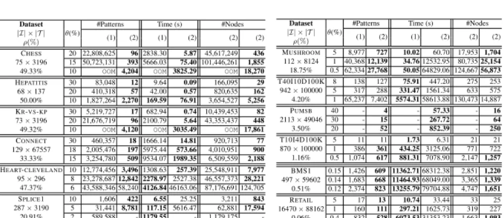
Table 1: CLOSEDDIV (Jmax = 0.05) vs CLOSEDP. For columns #Patterns and #Nodes, the
values in bold indicate a reduction more than 20% of the total number of patterns and nodes.“ − ” is shown when time limit is exceeded. OOM : Out Of Memory. (1): CLOSEDP (2): CLOSEDDIV
Experimental protocol. Experiments were carried out on classic UCI data sets, avail-able at the FIMI repository (fimi.ua.ac.be/data). We selected several real-world data sets, their characteristics (name, number of items |I|, number of transactions |T |, den-sity ρ) are shown in the first column of Table 1. We selected data sets of various size and density. Some data sets, such as Hepatitis and Chess, are very dense (resp. 50% and 49%). Others, such as T10 and Retail, are very sparse (resp. 1% and 0.06%). The implementation of the different global constraints and their constraint propagators were carried out in the Choco solver [17] version 4.0.3, a Java library for constraint pro-gramming. The source code is publicly available.5 Experiments were conducted on AMD Opteron 6174, 2.2 GHz with a RAM of 256 GB and a time limit of 24 hours. The default maximum heap size allowed by the JVM is 30 GB. We have selected for every data set frequency thresholds to have different numbers of frequent closed item-sets (|T h(c)| ≤ 15000, 30000 ≤ |T h(c)| ≤ 106, and |T h(c)| > 106). The only excep-tion are the very large and sparse data sets Retail and Pumsb, where we do not find a large number of solutions. We used the CLOSEDP CP model as a baseline to determine suitable thresholds used with the CLOSEDDIVCP model. To evaluate the quality of a set of patterns in terms of diversity, we measured the average ratio of exclusive pattern coverages: ECR(P1, ..., Pk) = avg1≤i≤k(
supD(Pi)−|VD(Pi) ∩Sj6=iVD(Pj)|
supD(Pi) ).
(a) Comparing CLOSEDDIV with CLOSEDP and FLEXICS. Table 1 compares the performance of the two CP models for various values of θ on different data sets. Here, we report the CPU time (in seconds), the number of extracted patterns, and the number of nodes explored during search. This enables to evaluate the amount of inconsistent values pruned by each approach (filtering algorithm). We use MINCOVas variable or-dering heuristic. The maximum diversity threshold Jmaxis set to 0.05. First, the results
highlight the great discrepancy between the two models with a distinctly lower number of patterns generated by CLOSEDDIV(in the thousands) in comparison to CLOSEDP (in the millions). On dense and moderately dense data sets (from CHESSto MUSHROOM),
the discrepancy is greatly amplified, especially for small values of θ. For instance, on CHESS, the number of patterns for CLOSEDDIV is reduced by 99% (from ∼ 50 · 106
solutions to 393) for θ equal to 15%. The density of the data sets provides an appro-priate explanation for the good performance of CLOSEDDIV. As the number of closed patterns increases with the density, redundancy among these patterns increases as well. On very sparse data sets, CLOSEDDIVstill outputs fewer solutions than CLOSEDP but the difference is less pronounced. This is explainable by the fact that on these data sets, where we have few solutions, almost all patterns are diverse.
Second, regarding runtime, CLOSEDDIV exhibits different behaviours. On dense data sets (ρ ≥ 30%), CLOSEDDIVis more efficient than CLOSEDP and up to an order of magnitude faster. On CHESS(resp. CONNECT), the speed-up is 1455 (resp. 112) for θ = 30%. For instances resulting in between 500 and 5000 diverse FCIs, the speed-up is speed-up to 5. This good performance of CLOSEDDIVis mainly due to the strength of the LB filtering rule that provides the CP solving process with more propagation to remove more inconsistent values in the search space. In addition, the number of nodes explored by CLOSEDDIVis always small comparing to CLOSEDP. These results sup-port our previous observations. The only exception is HEART-CLEVELANDfor which CLOSEDDIV is slower (especially for values of θ ≤ 8%). This is mainly due to the relative large number of diverse patterns (≥ 12000), which induces higher lower bound computational overhead. We observe the same behaviour on the two moderately dense data sets SPLICE1 and MUSHROOM. On sparse data sets, CLOSEDDIVcan take signif-icantly more time to extract all diverse FCIs. This can be explained by the fact that on these instances almost all FCIs are diverse w.r.t. lower bound (on average about 70% for RETAILand 39% for BMS1, see Table 1). Thus, non-solutions are rarely filtered, while the lower bound overhead greatly penalizes the CP solving process. On the very large PUMSB data set, finally, our approach is very efficient while CLOSEDP fails to complete the extraction.
Finally, Figure 2a compares CLOSEDDIVwith FLEXICS(two variants) for various values of θ on different data sets: GFLEXICS, which uses CP4IM [6] as an oracle to enumerate the solutions, and EFLEXICS, a specialized variant, based on ECLAT[23]. We run WEIGHTGENwith values of κ ∈ {0.1, 0.5, 0.9} [9]. For each instance, we fixed the number of samples to the number of solutions returned by CLOSEDDIV. We report results corresponding to the best setting of parameter κ. First, CLOSEDDIV largely dominates GFLEXICS, being more than an order of magnitude faster. Second, while EFLEXICSis faster than GFLEXICS, our approach is almost always ranked first, illus-trating its usefulness for mining diverse patterns in an anytime manner.
(b) Impact of varying Jmax. We varied Jmaxfrom 0.1 to 0.7. The minimum support
θ is fixed for each data set (indicated after ’-’). Figure 2 shows detailed results. As ex-pected, the greater Jmax, the longer the CPU time. In fact, the size of the history H
grows rapidly with the increase of Jmax. This induces significant additional costs in
the lower and upper bound computations. Moreover, when Jmaxbecomes sufficiently
large, the LB filtering of CLOSEDDIVoccurs rarely since the lower bound is almost al-ways below the Jmaxvalue (see Figure 3). Despite the hardness of some instances (i.e.,
Jmax≥ 0.35), our CP approach is able to complete the extraction for almost all values
(a) CPU-time MINCOVand FLEXICS (b) Moderately dense and sparse dat sets.
(c) Dense data sets.
Dataset θ(%)
Exclusive Coverage Ratio (ECR) CLOSEDP CLOSEDDIV–MINCOVEFLEXICS
T40I10D100K 8 1.6E-01 4.4E-01 1.29E-01 1 1.9E-01 9.2E-01 2.90E-01 SPLICE1 10 4.0E-02 1.6E-01 2.98E-02 5 4.0E-02 2.5E-01 1.79E-01 CONNECT 18 0.00 1.0E-01 4.31E-02 SPLICE1 10 4E-02 1.6E-01 2.98E-02 5 4E-2 2.5E-01 1.79E-01 CONNECT 18 1.25E-6 1.0E-01 4.31E-02 15 0.00 1.7E-01 4.16E-02 MUSHROOM 5 3.3E-4 5.6E-01 2.63E-01 1 3.73E-4 4.3E-01 4.2E-01 HEPATITIS 10 0.00 2.5E-01 1.0E-01 HEPATITIS 10 1.50E-3 2.5E-01 1.0E-01 T10I4D100K 1 5.9E-01 9.3E-01 5.72E-01 0.5 4.8E-01 9.6E-01 4.63E-01
(d) Patterns ECR.
Fig. 2: CPU-time analysis (MINCOVvs FIRSTWITCOVand CLOSEDDIVvs FLEXICS) and pat-terns discrepancy analysis.
to complete the extraction within the time limit for Jmax≥ 0.45. However, in practice,
the user will only be interested in small values of Jmaxbecause the diversity of patterns
is maximal and the number of patterns returned becomes manageable.
Figures 2b and 2c also compare the resolution time of our CP model using the two variable ordering heuristics MINCOV and FIRSTWITCOV. First, on dense data sets, both heuristics perform similarly, with a slight advantage for FIRSTWITCOV. On these data sets, the number of witness patterns mined remains very low (≤ 100), thus the benefits of FIRSTWITCOV is limited (see Supp. material). On moderately dense data sets (MUSHROOMand SPLICE1), FIRSTWITCOVis very effective; on MUSHROOMit is up 10 times faster than MINCOVfor Jmaxequal to 0.7. On these data sets, the number
of witness patterns extracted is relatively high compared to dense ones. In this case, FIRSTWITCOVenables to guide the search to find diverse patterns more quickly. On sparse data sets, no heuristic clearly dominates the other. When regarding the number of diverse patterns generated (see Supp. material), we observe that FIRSTWITCOVreturns less patterns on moderately dense and sparse data sets, while on dense data sets the number of diverse patterns extracted remains comparable.
(c) Qualitative analysis of the proposed relaxation. In this section, we shed light on the quality of the relaxation of the Jaccard constraint. Figure 3a shows, for a particular instance SPLICE1 with Jmax= 0.3, the evolution of the LBJand U BJof the solutions
(a) SPLICE1 (θ = 10%, Jmax= 0.3) (b) MUSHROOM(θ = 5%, Jmax= 0.7)
Fig. 3: Qualitative analysis of the LB and U B relaxations.
found during search. Here, the solutions are sorted according to their U BJ. Concerning
the lower bound, one can observe that the LBJ values are always below the Jmax
value. This shows how frequently the LB filtering rule of CLOSEDDIVoccurs. This also supports the suitability of the LB filtering rule for pruning non-diverse FCIs. With regard to the upper bound, it is interesting to see that it gets very close to the Jaccard value, meaning that our Jaccard upper bounding provides a tight relaxation. Moreover, a large number of solutions have U BJvalues either below or very close to Jmax. This is
indicative of the quality of the patterns found in terms of diversity. We recall that when U BJ< Jmax, all partial assignments can immediately be extended to diverse itemsets,
thanks to the anti-monotonicity property of our U B (see Proposition 5). We observe the same behaviour on MUSHROOMwith Jmax= 0.7 (see Figure. 3b). Finally, we can see
that FIRSTWITCOV allows to quickly discover solutions of better quality in terms of U BJ and Jaccard values compared to MINCOV. This demonstrates the interest and the
strength of our U BJbranching rule to get diverse patterns.
(d) Qualitative analysis of patterns. Figure 2d compares CLOSEDDIVwith CLOSEDP and EFLEXICSin terms of the ECR measure, which should be as high as possible. Due to the huge number of patterns generated by CLOSEDP, a random sample of k = 10 solutions of all patterns is considered. Reported values are the average over 100 trials. ECR penalises overlap, and thus having two similar patterns is undesirable. Accord-ing to ECR, leveragAccord-ing Jaccard in CLOSEDDIVclearly leads to pattern sets with more diversity among the patterns. This is indicative of patterns whose coverage are (ap-proximately) mutually exclusive. This should be desirable for an end-user tasked with exploring and interpreting the set of returned patterns.
7
Conclusions
In this paper, we showed that mining diverse patterns using a maximum Jaccard con-straint cannot be modeled using an anti-monotonic concon-straint. Thus, we have proposed (anti-)monotonic lower and upper bound relaxations, which allow to make pruning ef-fective, with an efficient branching rule, boosting the whole search process. The pro-posed approach is introduced as a global constraint called CLOSEDDIVwhere diversity is controlled through a threshold on the Jaccard similarity of pattern occurrences. Ex-perimental results on UCI datasets demonstrate that our approach significantly reduces
the number of patterns, the set of patterns is diverse and the computation time is lower compared to CLOSEDP global constraint, particularly on dense data sets.
References
1. Supplementary Material (June 2020), https://github.com/lobnury/ClosedDiversity.
2. Belaid, M., Bessiere, C., Lazaar, N.: Constraint programming for mining borders of frequent itemsets. In: Proceedings of IJCAI 2019, Macao, China. pp. 1064–1070 (2019)
3. Belfodil, A., Belfodil, A., Bendimerad, A., Lamarre, P., Robardet, C., Kaytoue, M., Plantevit, M.: Fssd-a fast and efficient algorithm for subgroup set discovery. In: Proceedings of DSAA. pp. 91–99 (2019)
4. Bosc, G., Boulicaut, J.F., Ra¨ıssi, C., Kaytoue, M.: Anytime discovery of a diverse set of patterns with monte carlo tree search. Data mining and knowledge discovery 32(3), 604–650 (2018)
5. Bringmann, B., Zimmermann, A.: The chosen few: On identifying valuable patterns. In: Proceedings of ICDM 2007. pp. 63–72
6. De Raedt, L., Guns, T., Nijssen, S.: Constraint programming for itemset mining. In: 14th ACM SIGKDD. pp. 204–212 (2008)
7. De Raedt, L., Zimmermann, A.: Constraint-based pattern set mining. In: 7th SIAM SDM. pp. 237–248. SIAM (2007)
8. Dzyuba, V., van Leeuwen, M., De Raedt, L.: Flexible constrained sampling with guarantees for pattern mining. Data Mining and Knowledge Discovery 31(5), 1266–1293 (2017) 9. Dzyuba, V., van Leeuwen, M.: Interactive discovery of interesting subgroup sets. In:
Inter-national Symposium on Intelligent Data Analysis. pp. 150–161. Springer (2013)
10. Hoeve, W., Katriel, I.: Global constraints. In: Handbook of Constraint Programming, pp. 169–208. Elsevier Science Inc. (2006)
11. Kifer, D., Gehrke, J., Bucila, C., White, W.: How to quickly find a witness. In: Constraint-Based Mining and Inductive Databases. pp. 216–242. Springer Berlin Heidelberg (2006) 12. Knobbe, A.J., Ho, E.K.: Pattern teams. In: Proceedings of ECML-PKDD. pp. 577–584.
Springer (2006)
13. Lazaar, N., Lebbah, Y., Loudni, S., Maamar, M., Lemi`ere, V., Bessiere, C., Boizumault, P.: A global constraint for closed frequent pattern mining. In: Proceedings of the 22nd CP. pp. 333–349 (2016)
14. van Leeuwen, M.: Interactive Data Exploration Using Pattern Mining, pp. 169–182. Springer Berlin Heidelberg, Berlin, Heidelberg (2014)
15. Ng, R.T., Lakshmanan, L.V.S., Han, J., Pang, A.: Exploratory mining and pruning optimiza-tions of constrained association rules. In: Proceedings of ACM SIGMOD. pp. 13–24 (1998) 16. Pei, J., Han, J., Lakshmanan, L.V.S.: Mining frequent item sets with convertible constraints.
In: Proceedings of ICDE. pp. 433–442 (2001)
17. Prud’homme, C., Fages, J.G., Lorca, X.: Choco Solver Documentation (2016)
18. Puolam¨aki, K., Kang, B., Lijffijt, J., De Bie, T.: Interactive visual data exploration with sub-jective feedback. In: Proceedings of ECML PKDD. pp. 214–229. Springer (2016)
19. Schaus, P., Aoga, J.O.R., Guns, T.: Coversize: A global constraint for frequency-based item-set mining. In: Proceedings of the 23rd CP 2017. pp. 529–546 (2017)
20. Van Leeuwen, M., Knobbe, A.: Diverse subgroup set discovery. Data Mining and Knowledge Discovery 25(2), 208–242 (2012)
21. Vreeken, J., Van Leeuwen, M., Siebes, A.: Krimp: mining itemsets that compress. Data Min-ing and Knowledge Discovery 23(1), 169–214 (2011)
22. Wang, J., Han, J., Pei, J.: CLOSET+: searching for the best strategies for mining frequent closed itemsets. In: Proceedings of the Ninth KDD. pp. 236–245. ACM (2003)
23. Zaki, M., Parthasarathy, S., Ogihara, M., Li, W.: New algorithms for fast discovery of associ-ation rules. In: Proceedings of KDD 1997, Newport Beach, California, USA, August 14-17, 1997. pp. 283–286. AAAI Press (1997)