Therapeutic target discovery using Boolean network attractors: improvements of kali

HAL Id: hal-01395079

https://hal.archives-ouvertes.fr/hal-01395079v3

Submitted on 8 Jan 2018

HAL is a multi-disciplinary open access

archive for the deposit and dissemination of

sci-entific research documents, whether they are

pub-lished or not. The documents may come from

teaching and research institutions in France or

abroad, or from public or private research centers.

L’archive ouverte pluridisciplinaire HAL, est

destinée au dépôt et à la diffusion de documents

scientifiques de niveau recherche, publiés ou non,

émanant des établissements d’enseignement et de

recherche français ou étrangers, des laboratoires

publics ou privés.

Therapeutic target discovery using Boolean network

attractors: improvements of kali

Arnaud Poret, Carito Guziolowski

To cite this version:

Arnaud Poret, Carito Guziolowski.

Therapeutic target discovery using Boolean network

at-tractors: improvements of kali.

Royal Society Open Science, The Royal Society, 2018, 5 (2),

�10.1098/rsos.171852�. �hal-01395079v3�

Therapeutic target discovery using Boolean

network attractors: improvements of kali

Arnaud Poret, Carito Guziolowski

January 8, 2018

Abstract

In a previous article, an algorithm for identifying therapeutic targets in Boolean networks modeling pathological mechanisms was introduced. In the present article, the improvements made on this algorithm, named kali, are described. These improvements are i) the possibility to work on asynchronous Boolean networks, ii) a finer assessment of therapeutic targets and iii) the possibility to use multivalued logic. kali assumes that the attractors of a dynamical system, such as a Boolean network, are as-sociated with the phenotypes of the modeled biological system. Given a logic-based model of pathological mechanisms, kali searches for thera-peutic targets able to reduce the reachability of the attractors associated with pathological phenotypes, thus reducing their likeliness. kali is illus-trated on an example network and used on a biological case study. The case study is a published logic-based model of bladder tumorigenesis from which kali returns consistent results. However, like any computational tool, kali can predict but can not replace human expertise: it is a sup-porting tool for coping with the complexity of biological systems in the field of drug discovery.

Copyright 2016-2018 Arnaud Poret

This article is licensed under the Creative Commons Attribution-NonCommercial-NoDerivatives 4.0 International License. To view a copy of this license, visit https://creativecommons.org/licenses/by-nc-nd/4.0/.

arnaud.poret@gmail.com (corresponding author) carito.guziolowski@ls2n.fr

LS2N, UMR 6004 Nantes, France

Contents

1 Introduction 3

1.1 Handling asynchronous updating . . . 3

1.2 Managing basin sizes for therapeutic purpose . . . 4

1.3 Extending to multivalued logic . . . 4

2 Methods 4 2.1 Additional definitions . . . 4

2.2 Handling asynchronous updating . . . 5

2.3 Managing basin sizes for therapeutic purpose . . . 5

2.4 Extending to multivalued logic . . . 6

2.5 Example network . . . 7

2.6 Case study: bladder tumorigenesis . . . 9

2.7 Implementation, code availability, license . . . 11

3 Results 11 3.1 Example network . . . 11

3.1.1 Attractor sets . . . 11

3.1.2 Therapeutic bullets . . . 12

3.2 Case study: bladder tumorigenesis . . . 15

3.2.1 Attractor sets . . . 15

3.2.2 Therapeutic bullets . . . 17

3.3 Computation times . . . 19

4 Conclusion 20 5 Appendix 1: recall of previous concepts 22 5.1 Biological networks . . . 22

5.2 Boolean networks . . . 22

5.3 Definitions . . . 23

6 Appendix 2: multivalued case 24 6.1 Attractor sets . . . 24

6.2 Therapeutic bullets . . . 25

7 Appendix 3: core of kali 28 7.1 Defined types . . . 28

7.2 Parameters . . . 28

7.3 Functions . . . 29

1

Introduction

In a previous article, an algorithm for in silico therapeutic target discovery was presented in its first version [1]. In the present article, the improvements made on this algorithm, named kali, are described. The complete background was introduced in the previous article whose some important concepts are recalled in Appendix 1 page 22.

kali still belongs to the logic-based modeling formalism [2–4], mainly Boolean networks [5, 6], and keeps its original goal: searching for therapeutic interven-tions aimed at healing a supplied pathologically disturbed biological network. Such a network is intended to model the biological mechanisms of a studied disease and is on what kali operates. Therapeutic interventions are combina-tions of targets, these combinacombina-tions being named bullets. Targets are network components, such as enzymes or transcription factors, and can be subjected to inhibition or activation. This is what bullets specify: which targets and which actions to apply on them.

The pivotal assumption on which kali is based postulates that the attrac-tors of a dynamical system, such as a Boolean network, are associated with the phenotypes of the modeled biological system. In other words: attractors model phenotypes [7]. This assumption was successfully applied in several works [8–14] and makes sense since the steady states of a dynamical system, the attractors, should mirror the steady states of the modeled biological system, the pheno-types.

In the mean time, various works using logical modeling with application in therapeutic innovation were published. An example is the work of Hyunho Chu and colleagues [15]. They built a molecular interaction network involved in colorectal tumorigenesis and studied its dynamics, particularly its attractors and their basins, with stochastic Boolean modeling. They highlighted what they termed the flickering, that is the displacement of the system from one basin to another one due to stochastic noise. They suggested that the flickering is involved in pushing the system from a physiological state to a pathological one during colorectal tumorigenesis.

Concerning kali, three improvements were done: i) adding the possibility to work with asynchronous Boolean networks, ii) implementing a finer assessment of therapeutic targets and iii) adding the possibility to use multivalued logic. The technical features resulting from these improvements are illustrated on a simple example network while their biological significance is assessed on a case study, namely a published logic-based model of bladder tumorigenesis [16].

1.1

Handling asynchronous updating

To compute the behavior of a discrete dynamical system, such as a Boolean network, its variables have to be iteratively updated. These iterative updates can be made synchronously or not [17]. If all the variables are simultaneously updated at each iteration then the network is synchronous, otherwise it is asyn-chronous. Compared to an asynchronous updating, the synchronous one is easier to compute. However, when the dynamics of a biological network is computed synchronously, it is assumed that all its components evolve simultaneously, an assumption which can be inappropriate according to what is modeled.

The asynchronous updating is frequently built so that one randomly selected

variable is updated at each iteration. This allows to capture two important features: i) biological entities do not necessarily evolve simultaneously and ii) noise due to randomness can affect when biological interactions take place [18– 20]. This is particularly true at the molecular scale, such as with signaling pathways, where macromolecular crowding and Brownian motion can impact the firing of biochemical reactions [21].

Therefore, the choice between a synchronous and an asynchronous updating may depend on the model, the computational resources and the acceptability of synchrony. Knowing that the luxury is to have the choice, kali can now use synchronous and asynchronous updating.

1.2

Managing basin sizes for therapeutic purpose

Until now, kali requires therapeutic bullets to remove all the attractors asso-ciated with pathological phenotypes, here named pathological attractors. This criterion for selecting therapeutic bullets is somewhat drastic. A smoother cri-terion should enable to consider more targeting strategies and then more possi-bilities for counteracting diseases. However, it could also unravel less effective therapeutic bullets, but being too demanding potentially leads to no results and the loss of nonetheless interesting findings.

The therapeutic potential of bullets could be assessed by estimating their ability at reducing the size of the pathological basins, namely the basins of pathological attractors. This criterion is more permissive since therapeutic bul-lets no longer have to necessarily remove the pathological attractors. Reducing the size of a pathological basin renders the corresponding pathological attractor less reachable and then the associated pathological phenotype less likely. This new criterion includes the previous one: removing an attractor means reducing its basin to the empty set. Consequently, therapeutic bullets obtainable with the previous criterion are still obtainable.

1.3

Extending to multivalued logic

One of the main limitations of Boolean models is that their variables can take only two values, which can be too simplistic in some cases. Depending on what is modeled, such as activity level of enzymes or abundance of gene products, considering more than two levels can be better. Without leaving the logic-based modeling formalism, one solution is to extend Boolean logic to multivalued logic [22].

With multivalued logic, a finite number h of values in the interval of real numbers [0; 1] is used, thus allowing variables to model more than two levels. For example, the level 0.5 can be introduced to model partial activation of enzymes or moderate concentration of gene products.

2

Methods

2.1

Additional definitions

In addition to the background introduced in the previous article [1] and briefly recalled in Appendix 1 page 22, here are some supplementary definitions:

• physiological state space: the state space Sphysio of the physiological

variant

• pathological state space: the state space Spatho of the pathological

variant

• testing state space: the state space Stest of the pathological variant

under the effect of a bullet

• physiological basin: the basin Bphysio,i of a physiological attractor

aphysio,i

• pathological basin: the basin Bpatho,iof a pathological attractor apatho,i

• n-bullet: a bullet made of n targets

2.2

Handling asynchronous updating

To incorporate asynchronous updating, the corresponding algorithms coming from BoolNet were implemented into kali. BoolNet is an R [23] package for gen-eration, reconstruction and analysis of Boolean networks [24]. Asynchronous updating is implemented so that one randomly selected variable is updated at each iteration. This random selection is made according to a uniform distribu-tion and implies that the network is no longer deterministic. To do so, given a Boolean network, BoolNet uses the three following functions:

• AsynchronousAttractorSearch: this function computes the attractor set of a supplied Boolean network by using the two following functions

• ForwardSet: this function computes the forward reachable set (see be-low) of a state and considers it as a candidate attractor

• ValidateAttractor: this function checks if a forward reachable set is a terminal strongly connected component (terminal SCC, see below), that is an attractor

The forward reachable set F wdx⊂ S of a state x ∈ S is the set made of the

states reachable from x, including x itself. A terminal SCC is a set tSCC ⊂ S made of the forward reachable sets of its states: ∀x ∈ tSCC, F wdx ⊂ tSCC.

As a consequence, when a terminal SCC is reached, the system can not escape it: this is an attractor in the sense of asynchronous Boolean networks [25].

Asynchronous Boolean networks with random updating are not determin-istic: their attractors are no longer deterministic sequences of states, namely cycles, but terminal SCCs. To find such an attractor, a long random walk is performed in order to reach an attractor with high probability. This candidate attractor is then validated, or not, by checking if it is a terminal SCC.

2.3

Managing basin sizes for therapeutic purpose

To implement the new criterion for selecting therapeutic bullets, kali consid-ers a bullet as therapeutic if it increases the union of the physiological basins S Bphysio,i in the testing state space Stest without creating de novo

attrac-tors. Knowing that for kali an attractor is either physiological or pathological, increasingS Bphysio,i is equivalent to decreasingS Bpatho,i.

The goal is to increase the physiological part of the pathological state space, or equivalently to decrease its pathological part. Consequently, a pathologically disturbed biological network receiving such a therapeutic bullet tends to, but not necessarily reaches, an overall physiological behavior.

However, as with the previous criterion, it does not ensure that all the phys-iological attractors are preserved. A fortiori, it does not ensure that their basin remains unchanged. It means that a therapeutic bullet can also alter the reach-ability of the physiological attractors. Nevertheless, as with the previous cri-terion, this is a matter of choice between a therapeutic bullet or no bullet at all.

The therapeutic potential of a bullet is expressed by its gain. It is displayed as follows:

x% → y% with x = 100 ·|S Bphysio,i| |Spatho|

and y = 100 ·|S Bphysio,i| |Stest|

expressed in percents. Therefore, in order to increase the physiological part of the pathological state space, a therapeutic bullet has to make y ≥ x.

Note that y = x is allowed. In this particular case, it is conceivable that the size of several pathological basins changed while the size of their union did not. In other words, the composition of the pathological part changed while its size did not. It can be therapeutic if, for example, the basin of a weakly pathological attractor increases at the expense of the basin of a heavily pathological attractor. The increase of the physiological part of the pathological state space can be subjected to a threshold δ: y ≥ x becomes y − x ≥ δ. As x and y, δ is expressed in percents of the state space. This threshold is introduced to allow the stringency of kali to be tuned. By the way, using this threshold also decreases the probability to obtain misassessed therapeutic bullets due to roundoff errors, or sampling errors when the state space is too big to compute trajectories from each of the possible states.

A therapeutic bullet as defined by the previous criterion, namely which re-moves all the pathological attractors, makes de facto S Bphysio,i = 100% of

Stest. As already mentioned, the previous criterion is included in this new one:

therapeutic bullets obtainable with the former are also obtainable with the lat-ter.

It must be pointed out that the current implementation of the method de-scribed in this article, namely kali, computes basin sizes by counting the number of initial states leading to a given attractor. If these initial states are a subset of the state space then basin sizes are estimations. Moreover, if an asynchronous updating is used then the system is not deterministic, implying that an initial state can lead to more than one attractor. Consequently, in those cases, basin sizes and therapeutic gains are estimations also subjected to random variations. In other words, concerning the calculation of basin sizes, the current imple-mentation of kali is more an attractor reachability estimation than a true basin size calculation. Nevertheless, speaking in terms of basins is kept in order to bet-ter comply with the underlaying method, independently of its implementation which is subjected to further improvements.

2.4

Extending to multivalued logic

Extending to multivalued logic requires suitable operators to be introduced. One solution is to use an implementation of the Boolean operators which also

works with multivalued logic, just as the Zadeh operators. These operators are a generalization of the Boolean ones proposed for fuzzy logic by its pioneer Lotfi Zadeh [26]. Their formulation is:

x ∧ y = min(x, y) x ∨ y = max(x, y)

¬x = 1 − x

With a h-valued logic, the size of the n-dimensional state space is hn, bring-ing more computational difficulties than with Boolean logic. The same applies to the testable bullets since there are hr possible modality arrangements and then (n! · hr)/(r! · (n − r)!) possible bullets, where r is the number of targets per bullet (see below).

As introduced in the previous article [1] and recalled in Appendix 1 page 22, a bullet is a couple (ctarg, cmoda) where ctarg= (targ1, . . . , targr) is a

com-bination without repetition of r nodes and cmoda = (moda1, . . . , modar) is an

arrangement with repetition of r perturbations, here termed modalities. modai

is intended to be applied on targi.

To illustrate how kali works with multivalued logic without overloading it, a 3-valued logic is used with {0, 0.5, 1} as domain of value: xi∈ {0, 0.5, 1}. 0 and

1 have the same meaning as with Boolean logic. 0.5 is an intermediate truth degree which can be interpreted as an intermediate level of activity/abundance depending on what the variables refer to. By the way, S = {0, 0.5, 1}n and modai∈ {0, 0.5, 1}.

2.5

Example network

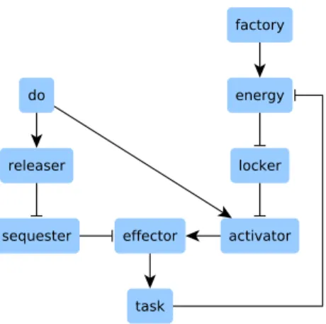
To conveniently illustrate the technical features resulting from the improvements made on kali, a simple and fictive example network is used. A biological case study is then proposed to address a concrete case, namely a published logic-based model of bladder tumorigenesis [16]. The example network is depicted in Figure 1 page 8.

Among the three improvements made on kali, only the asynchronous updat-ing and the management of basin sizes are illustrated. Multivalued logic is a straightforward extension of the Boolean case and is illustrated in Appendix 2 page 24. Below are the Boolean equations encoding the example network, also available in text format in the supporting file example_equations.txt:

do = do f actory = f actory

energy = f actory ∨ (energy ∧ ¬task) locker = ¬energy

releaser = do sequester = ¬releaser

activator = do ∧ ¬locker

ef f ector = activator ∧ ¬sequester task = ef f ector

Figure 1: This network, running in a fictive cell, controls the execution of a task according to two inputs: i) the do instruction, which tells the task to be performed, and ii) energy supply. The task consumes energy and must be prevented if no energy is available, even if the do instruction is sent. The task is initiated by an effector, which is maintained inactive by a sequester. The do instruction activates a releaser which suppresses the sequestering activity of the sequester, thus releasing the effector. However, to initiate the task and in addition to be released, the effector has also to be activated by an activator. When released and activated, the effector initiates the task. To ensure that the task is performed only if energy is available, a locker maintains the activator in an inactive state if there is no energy, even if the do instruction is sent. Concerning the factory, it supplies energy.

The do instruction and the factory are the two inputs: they are constant and therefore equal to themselves. The equation of energy tells that energy is present if the factory is active, even when the task is running: the factory has a sufficient production capacity. However, if the factory is not active then energy disappears as soon as the task is initiated. Concerning the activator and the effector, their equations tell that their respective inhibitor takes precedence: whatever is the state of the other nodes, if the inhibitor is active then the target is not.

The physiological variant fphysio is the network as is. The pathological

variant fpatho is the network plus a constitutive inactivation of the locker: the

execution of the task no longer considers if energy is available. Consequently, flockerbecomes locker = 0 in fpatho.

2.6

Case study: bladder tumorigenesis

The case study consists in running kali on a logic-based model of bladder tu-morigenesis published by Elisabeth Remy and colleagues [16]. Elisabeth Remy and colleagues have built an influence network linking three extracellular input signals and one intracellular input event to three cellular output phenotypes.

The three extracellular input signals are growth stimulations, represented by the EGF Rstimulus and F GF R3stimulus parameters, and growth inhibi-tions, mainly modeling TGF-β effects and represented by the GrowthInhibitors parameter. The intracellular input event is DNA damage, represented by the DN Adamage parameter. The three cellular output phenotypes are prolifera-tion, growth arrest and apoptosis. The model integrates downstream effectors of growth factor receptors such as Ras and PI3K, growth inhibitors such as p14ARF and p16INK4a, and regulators of the cell cycle such as cyclinD1, E2F3 and pRb.

Some variables are ternary: they can take three possible values in order to account for different effects depending on the activation level. These three possible values are 0 and 1 as in the Boolean case, plus the additional level 2. As in the model implementation performed by Elisabeth Remy and colleagues, these ternary variables are translated into pairs of Boolean variables: one Boolean variable per activation level, namely level 1 and level 2.

For example and according to the model, in its normal expression level (level 1, E2F 1 = 1) the transcription factor E2F1 stimulates the expression of genes supporting the cell cycle. However, when over-expressed (level 2, E2F 1 = 2) E2F1 stimulates the expression of genes supporting apoptosis. Consequently, this ternary variable is translated into the pair of Boolean variables E2F 1lvl1

and E2F 1lvl2:

E2F 1 = 1 ⇔ E2F 1lvl1= 1

E2F 1 = 2 ⇔ E2F 1lvl2= 1

The variable modeling the output phenotype Apoptosis is one of these ternary variables. The goal of Elisabeth Remy and colleagues was to relate apoptosis to its trigger: p53-dependent apoptosis (Apoptosislvl1) and E2F1-dependent

apoptosis (Apoptosislvl2). However, in the present case study, only the cell fate

matters. These two trigger-dependent apoptosis are therefore merged into one equation:

Apoptosis = Apoptosislvl1∨ Apoptosislvl2

Since the four inputs of the model are parameters, their respective value are directly injected into the concerned equations so that no equations are dedicated to them, thus reducing computational requirements. Again to reduce computa-tional requirements and knowing that the three output phenotypes are readouts not influencing other variables, their corresponding equation are put out of the model and evaluated from the returned attractors once the run terminated:

P rolif eration = CyclinE1 ∨ CyclinA GrowthArrest = p21CIP ∨ RB1 ∨ RBL2

Apoptosis = T P 53 ∨ E2F 1lvl2

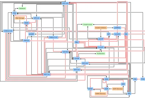
Altogether, the above described adaptations made on the model of bladder tumorigenesis by Elisabeth Remy and colleagues give a case study of 27 Boolean equations. These equations are listed in Appendix 4 page 36, also available in text format in the supporting file bladder_equations.txt. A network-based representation is shown in Figure 2 page 10.

Figure 2: A network-based representation of the case study used to assess kali on a concrete case. As explained in the text, it is derived from a published logic-based model of bladder tumorigenesis [16]. Nodes represent Boolean variables while edges indicate positive (black) and negative (red) influences. The input signals/events growth stimulations, growth inhibitions and DNA damage are in red while the output phenotypes proliferation, growth arrest and apoptosis are in green.

The physiological variant fphysiois the model as is. The pathological variant

f_patho is the model plus a deletion of the tumor suppressor gene CDKN2A, as observed in bladder cancers [27, 28]. Note that the CDKN2A gene encodes two growth inhibitors: p14ARF and p16INK4a. Consequently, the equations

modeling these two variables become p14ARF = 0 and p16IN K4a = 0 in f_patho.

2.7

Implementation, code availability, license

kali is implemented in Go [29], tested with Go version go1.9.2 linux/amd64 under Arch Linux [30]. kali is licensed under the GNU General Public License [31] and freely available on GitHub at https://github.com/arnaudporet/kali. The core of kali in pseudocode can be found in Appendix 3 page 28.

3

Results

3.1

Example network

3.1.1 Attractor sets

The example network is computed asynchronously over the whole state space, namely 512 possible initial states, using Boolean logic. As explained in the Methods section page 5, the asynchronous attractor search uses long random walks to reach candidate attractors with high probability, and then checks if they are indeed true attractors. Owing to the small size of the example network, the length maxk of these random walks is set to 1 000 steps. With larger state

spaces, random walks should be longer to reach candidate attractors with high probability.

The resulting attractors can be studied along four variables: the do instruc-tion, the factory, the locker and the task. It is possible for energy to be present without a running factory in the initial conditions. In this case, if the do instruc-tion is sent then energy is consumed by the task but not remade by the factory. With the physiological variant, the locker is expected to stop the task. However, with the pathological variant where the locker is disabled, an abnormal behavior is expected. Below are the computed attractors:

• Aphysio:

attractor basin (% of Sphysio) do f actory energy locker task

aphysio1 17.8% 0 0 0 1 0 aphysio2 7.2% 0 0 1 0 0 aphysio3 25% 0 1 1 0 0 aphysio4 25% 1 0 0 1 0 aphysio5 25% 1 1 1 0 1 • Apatho:

attractor basin (% of Spatho) do f actory energy locker task

apatho1 18.4% 0 0 0 0 0

aphysio2 6.6% 0 0 1 0 0

aphysio3 25% 0 1 1 0 0

apatho2 25% 1 0 0 0 1

aphysio5 25% 1 1 1 0 1

With the physiological variant, the behavior is as expected: the task runs only if the do instruction is sent and only if the factory can remade the consumed

energy. With the pathological variant, two pathological phenotypes represented by apatho1 and apatho2 appear. apatho1 is pathological because the locker is

inactive while there is no available energy. However, it is weakly pathological since the do instruction is not sent: there is no task to stop, an operational locker is not mandatory.

In contrast, apatho2 is heavily pathological because an operational locker is

required to stop the task in absence of energy supply. In the fictive cell bearing this example network, apatho2 could drain all its energy content, thus bringing

it to thermodynamical death. Moreover, apatho2 should not be neglected since

its basin occupies 25% of the pathological state space.

3.1.2 Therapeutic bullets

Bullets are assessed for their therapeutic potential on the pathological variant f_patho according to the new criterion: decreasing the size of the pathological basins Bpatho,i. All the bullets made of one to two targets are tested with a

threshold of 5%.

Choosing a threshold can appear somewhat arbitrary. It tells that if the physiological part S Bphysio,i in the pathological state space Spatho occupies

x% of it, then to be therapeutic a bullet has to bring this value above (x + 5)% in the testing state space Stest. Therefore, the increases below this threshold

are considered not significant by kali. Even the choice of using a threshold can be arbitrary, as discussed in the Methods section page 6.

Knowing thatS Bphysio,i= 56.6% of Spatho, with a threshold of 5% the 1,

2-bullets have to makeS Bphysio,i≥ (56.6+5)% = 61.6% of Stestto be considered

• 1-therapeutic bullets:

bullet gain Bphysio1 Bphysio2 Bphysio3 Bphysio4 Bphysio5 Bpatho1 Bpatho2

do[0] 56.6% → 64.4% 0% 14.4% 50% 0% 0% 35.5% 0% f actory[1] 56.6% → 100% 0% 0% 50% 0% 50% 0% 0%

• 2-therapeutic bullets:

bullet gain Bphysio1 Bphysio2 Bphysio3 Bphysio4 Bphysio5 Bpatho1 Bpatho2

do[0] f actory[1] 56.6% → 100% 0% 0% 100% 0% 0% 0% 0% do[1] f actory[1] 56.6% → 100% 0% 0% 0% 0% 100% 0% 0% do[0] energy[1] 56.6% → 100% 0% 50% 50% 0% 0% 0% 0% do[0] locker[0] 56.6% → 64.1% 0% 14.1% 50% 0% 0% 35.9% 0% do[0] releaser[0] 56.6% → 62.9% 0% 12.9% 50% 0% 0% 37.1% 0% do[0] sequester[1] 56.6% → 62.5% 0% 12.5% 50% 0% 0% 37.5% 0% do[0] activator[0] 56.6% → 64.8% 0% 14.8% 50% 0% 0% 35.2% 0% do[0] ef f ector[0] 56.6% → 67.8% 0% 17.8% 50% 0% 0% 32.2% 0% do[0] task[0] 56.6% → 73.2% 0% 23.2% 50% 0% 0% 26.8% 0% f actory[1] energy[1] 56.6% → 100% 0% 0% 50% 0% 50% 0% 0% f actory[1] locker[0] 56.6% → 100% 0% 0% 50% 0% 50% 0% 0%

where x[y] means that the variable x has to be set to the value y. For example, the therapeutic bullet do[0] f actory[1] suggests to abolish the do instruction while maintaining the factory active.

All the returned therapeutic bullets not removing all the pathological at-tractors exhibit the ability to suppress the basin of apatho2 while increasing the

one of apatho1. Certainly, removing all the pathological attractors should be

better, but knowing the apatho2 is more pathological than apatho1, such

ther-apeutic bullets can nevertheless be interesting. With the previous criterion, namely removing all the pathological attractors, these therapeutic bullets are not obtainable, thus highlighting fewer therapeutic strategies.

Some of the found therapeutic bullets enable physiological attractors re-quired by the pathological variant to react properly to the do instruction. For example, the therapeutic bullet f actory[1] enables aphysio3 and aphysio5,

cor-responding respectively to “no do, no task” and “do the task, energy supply”. However, the remaining of the therapeutic bullets, such as do[0] releaser[0] or do[1] f actory[1], either disable or force the do instruction, thus either suppress-ing or forcsuppress-ing the task. A network unable at performsuppress-ing the task or, at the opposite, permanently doing it may not be therapeutically interesting, even if energy is supplied.

None of the found therapeutic bullets suggest to reverse the constitutive in-activation of the locker. This highlights that applying the opposite action of a pathological disturbance is not necessarily a therapeutic solution, which can appear counterintuitive. This is because biological entities subjected to patho-logical disturbances belong to complex networks exhibiting behaviors which can not be predicted by mind [32, 33]. In such context, computational tools and their growing computing capabilities can help owing to their integrative power [34–38].

Also, none of the found therapeutic bullets allow the recovery of all the physiological attractors: there are no golden bullets. In a general manner, the components of biological networks should be able to take several states, such as enzymes which should be active when suitable. Consequently, healing a patho-logically disturbed biological network by maintaining some of its components in a particular state should not allow the recovery of a complete and healthy behavior. This is a limitation of the method implemented in kali.

This limitation is common in biomedicine while not necessarily being an issue. For example, statins are well known lipid-lowering drugs widely used in cardiovascular diseases with proven benefits [39, 40]. They inhibit an enzyme, the HMG-CoA reductase, and they do it constantly, just as the targets are modulated in the therapeutic bullets returned by kali. The HMG-CoA reductase is component of a complex metabolic network and maintaining it in an inhibited state should not allow this network to run properly, maybe causing some adverse effects. Nevertheless, such as with all drugs, this is a matter of benefit-risk ratio. All of this is to point that there are no perfect strategies for counteracting diseases and that computational tools, such as kali, can help scientists but can certainly not replace their expertise. Human expertise is mandatory to assess the returned predictions according to a concrete setting, and ultimately to take decisions.

3.2

Case study: bladder tumorigenesis

3.2.1 Attractor sets

The case study is computed asynchronously using Boolean logic. The state space being quite big with 134 217 728 possible states, to compute an attractor set kali performs random walks starting from 1 000 randomly selected initial states. A bigger state space also requires these random walks to be longer in order to reach candidate attractors with high probability. The length maxk of

the random walks is then increased to 10 000 steps.

The 4 input parameters of the model are tuned to simulate a biological situation where undamaged cells receive both growth stimulating and growth inhibiting signals from their environment:

EGF Rstimulus = 1 F GF R3stimulus = 1 GrowthInhibitors = 1 DN Adamage = 0

This input configuration aims at predicting the possible responses of the model to opposite growth instructions. In a cancerous setting, it is desirable that the growth inhibiting signal takes precedence over the stimulating one. With the pathological variant where the two growth inhibitors p14ARF and p16INK4a are absent, this desired precedence might be compromised in favor of tumorigenesis, thus correlating with the observed CDKN2A gene deletion in bladder cancers [27, 28].

The phenotypes associated with the returned attractors are evaluated using their respective equation once the run terminated, as explained in the Methods section page 10. Below are the computed attractors together with their pheno-types and basins, expressed in percents of the corresponding state space:

Aphysio Apatho

name aphysio1 aphysio2 aphysio3 aphysio1 apatho1

basin 10.7% 74.5% 14.8% 65.4% 34.6% phenotype GA GA P GA P AKT 0 0 0 0 0 AT Mlvl1 0 0 0 0 0 AT Mlvl2 0 0 0 0 0 CDC25A 0 0 1 0 1 CHEK1/2lvl1 0 0 0 0 0 CHEK1/2lvl2 0 0 0 0 0 CyclinA 0 0 1 0 1 CyclinD1 0 0 0 0 1 CyclinE1 0 0 1 0 1 E2F 1lvl1 0 0 1 0 1 E2F 1lvl2 0 0 0 0 0 E2F 3lvl1 0 1 1 0 1 E2F 3lvl2 0 0 0 0 0 EGF R 0 0 0 0 0 F GF R3 1 1 1 1 1 GRB2 0 0 0 0 0 M DM 2 0 0 0 0 0 p14ARF 0 0 1 0 0 p16IN K4a 0 1 1 0 0 p21CIP 1 1 0 1 0 P I3K 0 0 0 0 0 P T EN 0 0 0 0 0 RAS 1 1 1 1 1 RB1 1 0 0 1 0 RBL2 1 1 0 1 0 SP RY 1 1 1 1 1 T P 53 0 0 0 0 0

where GA means growth arrest and P means proliferation.

The physiological variant is able to exhibit the two possible responses ac-cording to the input configuration: proliferation, represented by aphysio3, and

growth arrest, represented by aphysio1 and aphysio2. Growth arrest occupies

85.2% of the physiological state space, suggesting that normal cells are more likely to comply with growth inhibiting signals than with stimulating ones.

With the pathological variant modeling cells whose the two growth inhibitors p14ARF and p16INK4a are lost, the two possible responses are still present with again growth arrest being more likely than proliferation. Even if aphysio2

disappears, growth arrest is still possible with aphysio1whose the basin increases

from 10.7% in Sphysio to 65.4% in Spatho. The proliferating phenotype is also

still possible but through the pathological attractor apatho1 which, in a way,

replaces the physiological attractor aphysio3.

However, the global tendency toward growth arrest significantly decreases: proliferation is more than twice likely in the pathological variant than in the physiological one with a shift from 14.8% in Sphysio to 34.6% in Spatho.

There-fore, such pathological cells might be less responsive to growth inhibiting signals and more apt at proliferating, which is a major concern in tumorigenesis and consistent with the loss of two growth inhibitors.

To ensure that browsing the state space by performing 1 000 random walks of 10 000 steps is sufficient to find all the attractors while estimating their

basin with little variability, the physiological and pathological attractor sets were computed 100 times each:

set attractor basin (% of S) Aphysio aphysio1 10.518 ± 0.833 aphysio2 73.462 ± 1.24 aphysio3 16.02 ± 1.091 Apatho aphysio1 65.037 ± 1.687 apatho1 34.963 ± 1.687

These results indicate that, in the present case study, browsing the state space by performing 1 000 random walks of 10 000 steps is enough robust to obtain reproducible results. Indeed, at each time, the same attractors are found: no attractor is missed. Moreover, the means of the basin estimations exhibit low standard deviations: basin estimations are subjected to variability but are nonetheless reliable.

3.2.2 Therapeutic bullets

As in the example network, bullets are assessed for their therapeutic potential on the pathological variant f_pathoaccording to the new criterion: increasing the physiological part S Bphysio,i in the testing state space Stest with a threshold

of 5%. It means that therapeutic bullets have to push S Bphysio,i from 65.4%

in Spatho to at least 65.4 + 5 = 70.4% in Stest.

This case study belonging to a cancerous setting, it is desirable that thera-peutic bullets also promote growth arrest in order to slow down tumorigenesis. In terms of basins and attractors, it means that interesting therapeutic bul-lets should decrease Bpatho1, avoid aphysio3, increase Bphysio1 and reintroduce

aphysio2. Such therapeutic bullets could be qualified as anti-proliferative.

All the 1 458 bullets made of one to two targets are tested. Among them, kali finds 9 1-therapeutic bullets and 174 2-therapeutic bullets listed in the support-ing files bladder_B_therap_1.txt and bladder_B_therap_2.txt respectively. In addition to increasing the physiological part, all the returned therapeutic bullets are anti-proliferative. Indeed, all of them do not reintroduce aphysio3

and decrease Bpatho1, thus promoting growth arrest through aphysio1 and/or

aphysio2.

For example, the two following 1-therapeutic bullets increase Bphysio1 while

decreasing Bpatho1, thus exhibiting anti-proliferative effect as expected when

targeting the well known growth promoting PI3K/Akt pathway [41]:

bullet gain Bphysio1 Bphysio2 Bphysio3 Bpatho1

AKT [0] 65.4% → 89.3% 89.3% 0% 0% 10.7% P I3K[0] 65.4% → 86% 86% 0% 0% 14%

Below is an other interesting 1-therapeutic bullet predicting that inhibiting CDC25A is anti-proliferative:

bullet gain Bphysio1 Bphysio2 Bphysio3 Bpatho1

CDC25A[0] 65.4% → 100% 100% 0% 0% 0%

This therapeutic bullet is able to definitively suppress proliferation by mak-ing Bphysio1 = 100% of Stest. It makes sense since the tyrosine phosphatase

CDC25A can activate several cyclin-dependent kinases (CDKs) which, with their cyclin partners, promote cell cycle and then growth [42]. This prediction

correlates with biological knowledge about CDC25A inhibitors as potential an-ticancer agents [43]. For example, it is demonstrated that inhibiting CDC25A can suppress the growth of hepatocellular carcinoma cells [44, 45]. Moreover, a recent work was specially dedicated to the synthesis of anticancer agents in-hibiting the CDC25A/B phosphatases [46].

This highlights that dry-lab predictions consistent with factual evidences coming from wet-lab experiments are obtainable through kali, provided that the underlaying model is consistent too. Note that this does not imply that all the predictions are correct: needless to say that biological interpretation by experts is still mandatory.

The 2-therapeutic bullets also bring some interesting predictions. For exam-ple, they indicate that sprouty (SPRY) could be a therapeutic target but only in combination with another one: there are no 1-therapeutic bullets containing it. Sprouty negatively regulates mitogen-activated protein kinase (MAPK) sig-naling pathways downstream of growth factor receptors and is down-regulated in many cancers [47]. Consequently, stimulating sprouty should be anti-proliferative and this is what suggest the two following therapeutic bullets, even if the gain is relatively minor:

bullet gain Bphysio1 Bphysio2 Bphysio3

Bpatho1

E2F 3lvl2[0] SP RY [1] 65.4% → 70.5% 70.5% 0% 0%

29.5%

M DM 2[0] SP RY [1] 65.4% → 71.7% 71.7% 0% 0% 28.3%

These two therapeutic bullets indicate that stimulating sprouty should be done along with an inhibition of MDM2 or E2F3. As with CDC25A, this pre-diction correlates with biological knowledge: MDM2 is a major inhibitor of the well known tumor suppressor p53 [48] while E2F3 is a required transcription factor for the cell cycle [49]. However, only the level 2 of E2F3 is concerned, meaning that only its over-expression should be prevented. In other words, this is not an inhibition of E2F3 but rather the prevention of its over-expression, if any.

In the returned therapeutic bullets there are also intriguing results such as the following one:

bullet gain Bphysio1 Bphysio2 Bphysio3 Bpatho1

F GF R3[1] 65.4% → 74.1% 74.1% 0% 0% 25.9%

This therapeutic bullet moderately increases Bphysio1at the expense of Bpatho1,

thus promoting growth arrest. However, FGFR3 is a growth factor receptor and is frequently subjected to activating mutations in low grade bladder cancers [50]. Therefore, stimulating FGFR3 should promote proliferation, not growth arrest. However, Elisabeth Remy and colleagues have implemented a negative crosstalk from FGFR3 to the growth factor receptor EGFR in their model. This negative crosstalk may explain why stimulating FGFR3 is predicted to be anti-proliferative.

Indeed, EGF R[0] is one of the returned therapeutic bullet and represent a direct inhibition of EGFR, a well studied target in cancer therapies [51, 52]. Consequently and according to the model, F GF R3[1] can be interpreted as an indirect inhibition of EGFR, especially since these two therapeutic bullets have almost identical effects in magnitude:

bullet gain Bphysio1 Bphysio2 Bphysio3 Bpatho1

EGF R[0] 65.4% → 75.4% 75.4% 0% 0% 24.6%

Finally, it should be noted that the three following bullets are not predicted therapeutic by kali: p14ARF [1], p16IN K4a[1] and p14ARF [1] p16IN K4a[1]. As with the example network, this suggests that applying the opposite action of the pathological disturbance is not necessarily a therapeutic solution. Moreover, and again as with the example network, none of the found therapeutic bullets allow the recovery of all the physiological attractors: golden bullets seem to be as idealistic as golden pills.

3.3

Computation times

The results presented in this article were obtained on a laptop with 16GB of RAM and an Intel Core i7-6600U processor. There are two kali parameters strongly influencing computation times. These two parameters control the at-tractor search and are:

• maxS: the maximum number of initial states to use when computing an

attractor set

• maxk: the length of the random walks performed to reach candidate

at-tractors

The asynchronous attractor search consists in performing maxS random

walks of maxk steps. Knowing that such a search is performed for computing

an attractor set and that one attractor set is computed per tested bullet, the computation time can greatly increase with maxS and/or maxk. By the way,

computation times also increase with ntarg, maxtarg and maxmoda, three kali

parameters controlling how much bullets are tested:

• ntarg: the number of targets per bullet

• maxtarg: the maximum number of target combinations to test

• maxmoda: the maximum number of modality arrangements to test

The used logic can also increase computation times because the size of the state space is hn, where n is the number of nodes in the network and h the number of possible values for the variables. For example, h = 2 with Boolean logic and h = 3 with 3-valued logic. h can also increase the number of testable bullets, and then computation times, since there are (n! · hntarg_)/(n

targ! · (n −

ntarg)!) possible bullets.

Below are the computation times of the runs performed for this article:

example network example network case study (Boolean) (3-valued) (Boolean) maxS 512 (all) 1 000 1 000

maxk 1 000 1 000 10 000

1-bullets 18 (all) 27 (all) 54 (all) 2-bullets 144 (all) 324 (all) 1 404 (all)

Aphysio 130ms 187ms 6s89ms

Apatho 109ms 218ms 6s55ms

Btherap (ntarg = 1) 2s510ms 6s775ms 5m57s950ms

Btherap (ntarg = 2) 19s133ms 1m23s526ms 2h43m36s709ms 19

4

Conclusion

kali can now work on both synchronous and asynchronous Boolean networks. This is probably the most required improvement since asynchronous updating is frequently used in the scientific community and might be better realistic than synchrony, as discussed in the Introduction section page 3. Consequently, a computational tool aimed at working on models built by the scientific commu-nity, such as kali, has to handle this updating scheme.

Also note that there are more than one asynchronous updating scheme. The one implemented in kali is the most popular and is named the general asyn-chronous updating: one randomly selected variable is updated at each iteration. However, other asynchronous updating methods exist. For example, with the random order updating, all the variables are updated at each iteration along a randomly selected order. Implementing various asynchronous updating schemes in kali could be a required future improvement.

kali now uses a new criterion for assessing therapeutic bullets. This new criterion brings a wider range of targeting strategies intended to push patho-logical behaviors toward physiopatho-logical ones. It is based on a more permissive assumption stating that reducing the reachability of pathological attractors is therapeutic.

For an in silico tool such as kali, being a little bit more permissive can be important since the findings obtained by simulations have to outlive the bottleneck separating predictions and reality. With a too strict assessment of therapeutic bullets, the risk of highlighting too few candidate targets or to miss some interesting ones can be high. Moreover, predicted does not necessarily mean true: a prediction of apparently poor interest can reveal itself of great interest, and vice versa.

This new criterion also brings a finer assessment of therapeutic bullets since all the possible increases ofS Bphysio,iin Stestare considered. With the previous

criterion, there was only one therapeutic potential: S Bphysio,i= 100% of Stest,

thus reducing the assessment of bullets to therapeutic or not. Things are not so dichotomous but rather nuanced: the assessment of therapeutic bullets should be nuanced too.

kali can now work with multivalued logic. Allowing variables to take an arbi-trary finite number of values should enable to more accurately model biological processes and produce more fine-tuned therapeutic bullets. However, this accu-racy and fine-tuning are at the cost of an increased computational requirement. Indeed, the size of the state space depends on the size of the model and the used logic.

Consequently, the size of the model and the used logic should be balanced: the smaller the model is, the more variables should be finely valued. For exam-ple, for an accurate therapeutic investigation, the model should only contain the essential and specific pieces of the studied pathological mechanisms modeled by a finely valued logic. On the other hand, for a broad therapeutic investigation, a more exhaustive model can be used but modeled by a coarse-grained logic.

Note that the ultimate multivalued logic is the infinitely valued one, which is fuzzy logic [53]. With fuzzy logic, the whole interval of real numbers [0; 1] is used to valuate variables, which might bring the best accuracy for the qualitative modeling formalism [54–56]. However, using such a continuous logic implies to leave the relatively convenient discrete paradigm to enter the continuous one

where, for example, the state space is infinite.

kali also demonstrates that it is able at predicting therapeutic bullets con-sistent with the underlaying model, with biological knowledge and with exper-imental evidences. For example, in the bladder tumorigensis case study, kali returned therapeutic bullets inhibiting the PI3K/Akt pathway or the CDC25A tyrosine phosphatase, two documented targets in cancer therapies.

Even the surprising F GF R3[1] therapeutic bullets, which suggests to stimu-late a growth factor receptor for promoting growth arrest, is consistent with the underlaying model. Indeed, according to this model, it appears that F GF R3[1] is founded in a negative crosstalk from FGFR3 to EGFR, thus indirectly in-hibiting the growth factor receptor EGFR, which is also a documented target in cancer therapies.

Two additional improvements are envisioned for kali. The first one is to allow therapeutic bullets to create new attractors, namely de novo attractors. It is conceivable that a bullet can greatly decrease pathological basins while creating a new attractor not belonging to the physiological variant nor to the pathological one. Such a de novo attractor is currently tagged by kali as not physiological and then pathological, thus rejecting the concerned bullet. However, if a de novo attractor is weakly pathological and induced by a bullet greatly decreasing the basin of other and heavier pathological attractors, such a case should be retained.

The second envisioned improvement is to allow partial matching when check-ing if an attractor is associated with a physiological phenotype by comparcheck-ing it to the physiological attractors. Currently, an attractor which does not match a physiological attractor is considered pathologic. However, it is conceivable that some variables not exhibiting a physiological behavior in an attractor do not pathologically impact its associated phenotype. To allow such a case to be con-sidered, some variables within attractors should be allowed to not be matched when assessing the associated phenotype.

This suggests the concept of decisive variables, namely variables whose the behavior in the attractors is sufficient to biologically interpret the associated phenotypes. Elisabeth Remy and colleagues have already implemented this distinction in their model of bladder tumorigenesis used in the present article as case study: decisive variables are those belonging to the equations of the three output phenotypes. Therefore, kali could allow non-decisive variables to not be matched.

Ultimately, this could allow the modeler to specify himself/herself what a physiological attractor is without having to consider a physiological and a patho-logical variant. This could also allow to no longer think in terms of physiopatho-logical versus pathological attractors but just desirable ones. Moreover, implementing the second envisioned improvement could greatly facilitate the implementation of the first one since the goal would become to obtain desired attractors regard-less if they are de novo or not.

5

Appendix 1: recall of previous concepts

Below are some important concepts introduced in the previous article where the complete background was presented [1].

5.1

Biological networks

A network is a directed graph G = (V, E) where V = {v1, . . . , vn} is the set

containing the nodes of the network and E = {(vi,1, vj,1), . . . , (vi,m, vj,m)} is the

set containing the edges linking these nodes. In practice, nodes represent entities while edges represent binary relations R ⊂ V2_{involving them: v}

i R vj [57]. It

indicates that the node vi exerts an influence on the node vj. For example, in

gene regulatory networks [58], vi can be a transcription factor while vj a gene

product. The edges are frequently signed so that they indicate if vi exerts a

positive or a negative influence on vj, such as an activation or an inhibition.

5.2

Boolean networks

A Boolean network is a network where nodes are Boolean variables xiand edges

(xi, xj) are the is input of relation: xi is input of xj. Each variable xi has

bi ∈ [[0, n]] inputs influencing its state. Note that bi = 0 is possible. In this

case, xi is an input of the network. Depending on the updating scheme, at

each iteration k ∈ [[k0, kend]] one or more xi are updated using their associated

Boolean transition function fi. This function uses Boolean operators, typically

∧ (and), ∨ (or) and ¬ (not), to specify how the inputs xi,1, . . . , xi,bi of xi have

to be related to compute its value, as in the following pseudocode representing a synchronous updating: for k ← k0, . . . , kend x1← f1(x1,1, . . . , x1,b1) .. . xn← fn(xn,1, . . . , xn,bn) end for

which can be written in a more concise form:

for k ← k0, . . . , kend

x ← f (x) end for

where f = (f1, . . . , fn) is the Boolean transition function of the network and

x = (x1, . . . , xn) is its state vector. The value of the state vector belongs to the

state space S = {0, 1}n, which is the set containing all the possible states of the network.

The set A = {a1, . . . , ap} containing the attractors of the network is its

attractor set. An attractor ai is a collection of states (x1, . . . , xq) such that

once the system reaches a state xj ∈ ai, it can subsequently visit the states of

aibut no other ones: the system can not escape. The set Bi⊂ S containing the

states x ∈ S from which ai can be reached is its basin of attraction, or simply

5.3

Definitions

• physiological phenotype: a phenotype which does not impair the life quantity/quality of the organism which exhibits it

• pathological phenotype: a phenotype which impairs the life quantity/ quality of the organism which exhibits it

• variant (of a biological network): given a biological network, a variant is one of its versions, namely the network plus eventually some modifica-tions

• physiological variant: a variant which produces only physiological phe-notypes, this is the biological network as it should be, the one of healthy organisms

• pathological variant: a variant which produces at least one pathological phenotype, this is a dysfunctional version of the biological network, a version found in ill organisms

• physiological attractor set: the attractor set Aphysio of the

physiolog-ical variant

• pathological attractor set: the attractor set Apathoof the pathological

variant

• physiological Boolean transition function: the Boolean transition function f_physio of the physiological variant

• pathological Boolean transition function: the Boolean transition function f_patho of the pathological variant

• physiological attractor: an attractor ai such that ai ∈ Aphysio, note

that it does not exclude the possibility that ai ∈ Apatho in addition to

ai ∈ Aphysio

• pathological attractor: an attractor ai such that ai∈ A/ physio

• modality: the perturbation modai ∈ {0, 1} applied on a node vj of the

network, either activating (modai = 1) or inactivating (modai = 0), at

each iteration modai overwrites fj(x) making xj = modai

• target: a node targiof the network on which a modality modaiis applied

• bullet: a couple (ctarg, cmoda) where ctarg = (targ1, . . . , targr) is a

com-bination without repetition of r targets and cmoda= (moda1, . . . , modar)

is an arrangement with repetition of r modalities, modaiis intended to be

applied on targi

6

Appendix 2: multivalued case

Below is the multivalued version of the example network:

do = do f actory = f actory

energy = max(min(energy, 1 − task), f actory) locker = 1 − energy

releaser = do

sequester = 1 − releaser activator = min(do, 1 − locker)

ef f ector = min(activator, 1 − sequester) task = ef f ector

where the Boolean operators are replaced by the Zadeh ones.

To take advantage of multivalued logic, flocker becomes locker = min(1 −

energy, 0.5) in fpatho. This equation tells that the locker is actionable when

required, namely when there is no energy, but that it is unable at being fully operational due to some pathological defects: the maximal value of flocker in

f_patho is 0.5.

As mentioned in the article, 0.5 can be interpreted as an incomplete activa-tion/inhibition depending on what is modeled. Consequently, in the pathological variant, the activator is at most partly inhibited by the locker when no energy is available, allowing the task to be nevertheless performed. However, in this case, the task is itself moderately performed.

6.1

Attractor sets

The example network is computed asynchronously using a 3-valued logic. To compute an attractor set, kali performs 1 000 random walks of 1 000 steps. Below are the returned attractors:

• Aphysio:

attractor basin (% of Sphysio) do f actory energy locker task

aphysio1 6.1% 0 0 0 1 0 aphysio2 4.5% 0 0 0.5 0.5 0 aphysio3 2.5% 0 0 1 0 0 aphysio4 9.7% 0 0.5 0.5 0.5 0 aphysio5 1.8% 0 0.5 1 0 0 aphysio6 10.8% 0 1 1 0 0 aphysio7 6.5% 0.5 0 0 1 0 aphysio8 4.8% 0.5 0 0.5 0.5 0.5 aphysio9 10.3% 0.5 0.5 0.5 0.5 0.5 aphysio10 10.6% 0.5 1 1 0 0.5 aphysio11 7.3% 1 0 0 1 0 aphysio12 3.2% 1 0 0.5 0.5 0.5 aphysio13 10.3% 1 0.5 0.5 0.5 0.5 aphysio14 11.6% 1 1 1 0 1 • Apatho:

attractor basin (% of Spatho) do f actory energy locker task apatho1 6.2% 0 0 0 0.5 0 aphysio2 4.7% 0 0 0.5 0.5 0 aphysio3 2.2% 0 0 1 0 0 aphysio4 9.7% 0 0.5 0.5 0.5 0 aphysio5 1.8% 0 0.5 1 0 0 aphysio6 10.8% 0 1 1 0 0 apatho2 5.5% 0.5 0 0 0.5 0.5 aphysio8 5.8% 0.5 0 0.5 0.5 0.5 aphysio9 10.3% 0.5 0.5 0.5 0.5 0.5 aphysio10 10.6% 0.5 1 1 0 0.5 apatho3 7.3% 1 0 0 0.5 0.5 aphysio12 3.2% 1 0 0.5 0.5 0.5 aphysio13 10.3% 1 0.5 0.5 0.5 0.5 aphysio14 11.6% 1 1 1 0 1 aphysio1, aphysio3, aphysio6, aphysio11 and aphysio14 are the physiological

at-tractors found in the Boolean case with a different numbering due to additional attractors coming from multivalued logic. Indeed, given that {0, 1} ⊂ {0, 0.5, 1} and that the Zadeh operators also work with Boolean logic, the Boolean results are still obtainable. The same does not apply to the pathological attractors because flocker in fpatho differs between the Boolean and multivalued cases.

For example, aphysio13indicates that the do instruction is sent while energy

is partly supplied. Consequently, the locker is partly activated resulting in a partial inhibition of the activator. The task is thus moderately performed despite full do instruction, hence coping with moderate energy supply.

Concerning the pathological attractors, as an example apatho3indicates that

the do instruction is sent in absence of energy supply. Consequently, the locker should be fully activated to prevent the task. However, due to some pathological defects, the locker is at most partly activated. The task is then performed in absence of energy. However, since the locker is partly operational, the task is not performed at its maximum rate, maybe limiting pathological consequences. Among the pathological attractors, apatho1can be considered weakly

patho-logical. Indeed, in apatho1 the locker should be fully activated since there is

no energy. However, there is no do instruction and therefore no task to stop. On the other hand, apatho2 and apatho3 are more pathological since the task is

performed while no energy is available.

6.2

Therapeutic bullets

All the bullets made of one to two targets are tested with a threshold of 5%. Below are the returned therapeutic bullets:

• 1-therapeutic bullets:

bullet gain Bphysio1 Bphysio2 Bphysio3 Bphysio4 Bphysio5 Bphysio6 Bphysio7 Bphysio8 Bphysio9 Bphysio10 Bphysio11 Bphysio12 Bphysio13 Bphysio14 Bpatho1 Bpatho2 Bpatho3

f actory[0.5] 81% → 100% 0% 0% 0% 29.3% 6.1% 0% 0% 0% 32.2% 0% 0% 0% 32.4% 0% 0% 0% 0%

f actory[1] 81% → 100% 0% 0% 0% 0% 0% 35.4% 0% 0% 0% 32.2% 0% 0% 0% 32.4% 0% 0% 0%

• 2-therapeutic bullets:

bullet gain Bphysio1 Bphysio2 Bphysio3 Bphysio4 Bphysio5 Bphysio6 Bphysio7 Bphysio8 Bphysio9 Bphysio10 Bphysio11 Bphysio12 Bphysio13 Bphysio14 Bpatho1 Bpatho2 Bpatho3

do[0] f actory[0.5] 81% → 100% 0% 0% 0% 84% 16% 0% 0% 0% 0% 0% 0% 0% 0% 0% 0% 0% 0% do[0] f actory[1] 81% → 100% 0% 0% 0% 0% 0% 100% 0% 0% 0% 0% 0% 0% 0% 0% 0% 0% 0% do[0.5] f actory[0.5] 81% → 100% 0% 0% 0% 0% 0% 0% 0% 0% 100% 0% 0% 0% 0% 0% 0% 0% 0% do[0.5] f actory[1] 81% → 100% 0% 0% 0% 0% 0% 0% 0% 0% 0% 100% 0% 0% 0% 0% 0% 0% 0% do[1] f actory[0.5] 81% → 100% 0% 0% 0% 0% 0% 0% 0% 0% 0% 0% 0% 0% 100% 0% 0% 0% 0% do[1] f actory[1] 81% → 100% 0% 0% 0% 0% 0% 0% 0% 0% 0% 0% 0% 0% 0% 100% 0% 0% 0% do[0] energy[1] 81% → 100% 0% 0% 34.9% 0% 32.1% 33% 0% 0% 0% 0% 0% 0% 0% 0% 0% 0% 0% do[0] task[0] 81% → 89% 0% 11.6% 12.3% 21.3% 10.8% 33% 0% 0% 0% 0% 0% 0% 0% 0% 11% 0% 0% do[0.5] task[0.5] 81% → 89.4% 0% 0% 0% 0% 0% 0% 0% 24.3% 32.1% 33% 0% 0% 0% 0% 0% 10.6% 0% f actory[0] energy[0.5] 81% → 100% 0% 35.4% 0% 0% 0% 0% 0% 32.2% 0% 0% 0% 32.4% 0% 0% 0% 0% 0% f actory[0.5] energy[0.5] 81% → 100% 0% 0% 0% 35.4% 0% 0% 0% 0% 32.2% 0% 0% 0% 32.4% 0% 0% 0% 0% f actory[1] energy[1] 81% → 100% 0% 0% 0% 0% 0% 35.4% 0% 0% 0% 32.2% 0% 0% 0% 32.4% 0% 0% 0% f actory[1] locker[0] 81% → 100% 0% 0% 0% 0% 0% 35.4% 0% 0% 0% 32.2% 0% 0% 0% 32.4% 0% 0% 0% 26

For example, the therapeutic bullet f actory[1] locker[0] is interesting. It suppresses all the pathological attractors while maintaining three physiological attractors allowing the pathological variant to properly respond to the three possible levels of the do instruction. Moreover, the basins of these three phys-iological attractors, namely aphysio6, aphysio10 and aphysio14, equally span the

state space, making them equally reachable.

On the other hand, the therapeutic bullet do[0.5] f actory[0.5] seems to be less interesting. While this bullet also suppresses all the pathological attrac-tors, it enables only one physiological attractor. In this physiological attractor, namely aphysio9, all the variables are at their intermediate level: the network

can not fulfill its switching function.

7

Appendix 3: core of kali

Below is the core of kali in pseudocode derived from its Go [29] sources, freely available on GitHub at https://github.com/arnaudporet/kali under the GNU General Public License [31]. Note that the code may have evolved since the publication of the present article.

7.1

Defined types

structure Attractor// an attractor

field N ame// its name, either aphysio or apatho

field Basin// the size of its basin, in percents of the state space

field States// its states, as a matrix of one state per row

end structure

structure Bullet// a bullet

field T arg// its target combination, as a vector

field M oda// its modality arrangement, as a vector

field Gain// its gain, see below

field Cover// the size of each basin under its influence, see below

end structure

b.Gain is a vector (gain1, gain2) where:

• gain1 is the size ofS Bphysio,i in Spatho

• gain2 is the size ofS Bphysio,i in Stest

in % of Spatho and % of Stest respectively.

b.Cover is a vector containing the size of the physiological and pathological basins in the testing state space, in percents of it.

7.2

Parameters

nodes// the node names, as a vector

Ω// the domain of the used logic, as a vector

sync// use synchronous updating (sync = 1) or not (sync = 0)

whole// build the whole state space (whole = 1) or not (whole = 0)

maxS// the maximal size of the state space sample when whole = 0

maxk// the number of steps for the random walks (asynchronous only)

ntarg// the number of targets per bullet

maxtarg// the maximum number of target combinations to test

maxmoda// the maximum number of modality arrangements to test

δ// the threshold for a bullet to be therapeutic, in percents of the state space

When whole = 0, a subset of the state space is built. This subset contains the initial states from which trajectories are performed. These trajectories are used for computing an attractor set, that is to reach the attractors. Note that these trajectories are free to evolve in all the state space. In other words, kali does

not run on a subset of the state space, these are the initial states which are a subset of the state space.

To be considered therapeutic, a bullet has to make gain2− gain1≥ δ while not

creating de novo attractors.

7.3

Functions

function DoT heJ ob(fphysio, fpatho, ntarg, maxtarg, maxmoda, maxS, maxk, δ,

sync, nodes, Ω, whole)

// do the job, this is the main function

n ← Size(nodes)// the dimension of the state space S

select whole

case 0// build a sample of S

S ← GenArrangs(Ω, n, maxS)

case 1// build all S

S ← GenSpace(Ω, n) end select

Aphysio← ComputeAttractorSet(fphysio, S, ∅, maxk, 0, sync, ∅)

Apatho← ComputeAttractorSet(fpatho, S, ∅, maxk, 1, sync, Aphysio)

Aversus← GetV ersus(Apatho)// the pathological attractors, see below

Ctarg← GenCombis({1, . . . , n}, ntarg, maxtarg)// the target combinations

Cmoda← GenArrangs(Ω, ntarg, maxmoda)// the modality arrangements

if Aversus 6= ∅// there are pathological basins to shrink

Btherap← ComputeT herapeuticBullets(fpatho, S, Ctarg, Cmoda, maxk,

δ, sync, Aphysio, Apatho, Aversus)// therapeutic bullets

end if

return S, Aphysio, Apatho, Aversus, Ctarg, Cmoda, Btherap

end function

Size(container) returns the number of items in container.

GenSpace(Ω, n) returns the n-dimensional state space of the vectors made of n values from Ω, as a matrix of one state vector per row.

GenArrangs(Ω, n, maxarrang) returns maxarrang arrangements with repetition

made of n elements from Ω, as a matrix of one arrangement per row. If maxarrangexceeds its maximal possible value then it is automatically decreased

to its maximal possible value.

GenCombis(Ω, n, maxcombi) returns maxcombi combinations without repetition

made of n elements from Ω, as a matrix of one combination per row. If maxcombi

exceeds its maximal possible value then it is automatically decreased to its max-imal possible value.

As explained later, the function ComputeAttractorSet can use an already com-puted attractor set, namely the reference set, to name the attractors.

Aphysio is computed without bullet (b ← ∅), without reference set (Aref ← ∅)

and with the physiological setting (setting ← 0).

Apatho is computed without bullet (b ← ∅), with a reference set (Aref ←

Aphysio) and with the pathological setting (setting ← 1).

Aversus is not a true attractor set but the set containing the pathological

at-tractors: Aversus ⊂ Apatho. Apatho can contains physiological attractors if the

pathological variant exhibits some of them. However, Aversusonly contains the

pathological attractors.

Therapeutic bullets are computed only if there are pathological basins to shrink, namely only if Aversus6= ∅.

Note that target combinations are combinations of positions in the state vec-tor: targets are identified by their position in the state vector, not by their name.

function fphysio(x)

// update the state vector of the physiological variant

y[1] ← fphysio[1](x)// update x1with fphysio,1

.. .

y[n] ← fphysio[n](x)// update xn with fphysio,n

return y// the updated state vector

end function

function fpatho(x)

// update the state vector of the pathological variant

y[1] ← fpatho[1](x)// update x1 with fpatho,1

.. .

y[n] ← fpatho[n](x)// update xn with fpatho,n

return y// the updated state vector

end function

function ComputeAttractor(f, x0, b, maxk, sync)

// from x0, reach an attractor a

select sync

case 1// search a cycle

a.States ← ReachCycle(f, x0, b)

case 0// search a terminal SCC

for

a.States ← GoF orward(f, W alk(f, x0, b, maxk), b)// a candidate

if IsT erminal(a, f, b)// the candidate attractor is a terminal SCC

break// then it is an asynchronous attractor

end if end for end select return a end function

If ComputeAttractor(f, x0, b, maxk, sync) is run with sync = 0 (i.e.

asyn-chronous case) then ensure that maxk is big enough for random walks to reach

attractors with high probability. If maxkis too small and if there is no attractor

near x0, then this function will run indefinitely since it loops until an attractor

is found starting from x0. The default value of maxk should be 10 000. It can

be smaller for little networks and should be higher for large networks.

function ComputeAttractorSet(f, S, b, maxk, setting, sync, Aref)

// compute an attractor set A, namely Aphysio, Apatho or Atest

A ← {}

select setting// select the default name for attractors

case 0// physiological setting

name ← aphysio

case 1// pathological setting

name ← apatho

end select

for i ← 1, . . . , Size(S)// browse S

a ← ComputeAttractor(f, S[i], b, maxk, sync)

if ∃iA: A[iA] = a// a is already found

A[iA].Basin ← A[iA].Basin + 1// then increase its basin

else// new attractor

a.Basin ← 1// then begin its basin

A ← A ∪ {a}// and add it to the attractor set

end if end for

for i ← 1, . . . , Size(A)// browse A

A[i].Basin ← 100 · A[i].Basin/Size(S)// translate basins to % of S

end for

return SetN ames(A, name, Aref)// return named attractors, see later

end function

function ComputeT herapeuticBullets(fpatho, S, Ctarg, Cmoda, maxk, δ, sync,

Aphysio, Apatho, Aversus)

// compute a set Btherap of therapeutic bullets

Btherap← {}

b.Gain[1] ← Sum(GetCover(Aphysio, Apatho))//S Bphysio,i in Spatho

for i1← 1, . . . , Size(Ctarg)// browse the target combinations to test

for i2← 1, . . . , Size(CM oda)// browse the modality arrangements to test

b.T arg ← Ctarg[i1]// the target combination to test

b.M oda ← CM oda[i2]// the modality arrangement to test

Atest← ComputeAttractorSet(fpatho, S, b, maxk, 1, sync, Aphysio)

b.Gain[2] ← Sum(GetCover(Aphysio, Atest))//S Bphysio,i in Stest

if IsT herapeutic(b, Atest, Aversus, δ)// b is therapeutic

b.Cover ← GetCover(Aphysio∪ Aversus, Atest)// basins in Stest

Btherap← Btherap∪ {b}// add b to the set of therapeutic bullets

end if end for end for return Btherap

end function

Sum(container) returns the sum of the items in container.

function GetCover(A1, A2)

// get the size of the B1,iin S2, in % of S2

cover ← ()

for i1← 1, . . . , Size(A1)// browse the attractors of A1

if ∃i2: A2[i2] = A1[i1]// A1[i1] also in A2

cover ← Append(cover, A2[i2].Basin)// get the size of B1,i1 in S2

else// A1[i1] not in A2

cover ← Append(cover, 0)// then B1,i1 is empty in S2

end if end for return cover end function

Append(container, item) returns container with item added to it.

function GetV ersus(Apatho)

// get the pathological attractors

Aversus← {}// the set of the pathological attractors

for i ← 1, . . . , Size(Apatho)// browse the attractors of Apatho

if IsSubString(Apatho[i].N ame, patho)// not a physiological attractor

Aversus← Aversus∪ {Apatho[i]}// then add it to Aversus

end if end for return Aversus

end function

IsSubString(s1, s2) returns true if s2 is a substring of s1.

Remember that Aversus is not a true attractor set but the set containing the

pathological attractors: Aversus⊂ Apatho.

function GoF orward(f, x0, b)

// compute the forward reachable set f wd of x0 (asynchronous only)

f wd ← {x0}// f wd contains x0itself

stack ← (x0)// the stack of the states to check, see below

for

x ← stack[Size(stack)]// get the last stack element

stack ← stack[1, . . . , Size(stack) − 1]// remove the last stack element

y ← f (x)// prepare all the updated xi

for i ← 1, . . . , Size(y)// browse the updated xi

z ← x// copy x to preserve its original value

z[i] ← y[i]// update only one xi

z ← Shoot(z, b)// apply the bullet

if z /∈ f wd// new state

f wd ← f wd ∪ {z}// then add it to f wd