HAL Id: hal-01007128
https://hal.archives-ouvertes.fr/hal-01007128
Submitted on 24 Nov 2016
HAL is a multi-disciplinary open access
archive for the deposit and dissemination of
sci-entific research documents, whether they are
pub-lished or not. The documents may come from
teaching and research institutions in France or
L’archive ouverte pluridisciplinaire HAL, est
destinée au dépôt et à la diffusion de documents
scientifiques de niveau recherche, publiés ou non,
émanant des établissements d’enseignement et de
recherche français ou étrangers, des laboratoires
Numerical simulation of CAD thin structures using the
eXtended Finite Element Method and Level Sets
Grégory Legrain, Christophe Geuzaine, J. F. Remacle, Nicolas Moës, P.
Cresta, J. Gaudin
To cite this version:
Grégory Legrain, Christophe Geuzaine, J. F. Remacle, Nicolas Moës, P. Cresta, et al.. Numerical
simulation of CAD thin structures using the eXtended Finite Element Method and Level Sets. Finite
Elements in Analysis and Design, Elsevier, 2013, 77, pp.40-58. �10.1016/j.finel.2013.08.007�.
�hal-01007128�
1. Introduction
The assessment of the mechanical behaviour of complex industrial parts is still an issue nowa-days. Usually, these parts are composed of both thin and massive areas that are assembled together along junctions. The mechanical behaviour of these massive and thin areas is different, so that different models are usually considered. The usual path for such analysis begin with the CAD representation of the structure: both thin and thick areas are represented as three-dimensional volumes which are described by their outer boundary (BREP). This volumetric representation is converted into plates or shells by means of the extraction of the mid-plane of the part. Extracting this mid-plane cannot always be automatized for complex shapes, leading to some tedious and time consuming issues (difficulties to obtain continuous mid-planes with part assembly). However, the constitutive equations must also be rewritten for plate and shells models, which can be problematic for non-linear problems. Moreover, a special care as to be taken on the junction between these 2D zones and the 3D massive parts. Usually, the kinematic link between the two areas induces stress concentrations. This is why in some highly secured applications, solid modelizations have to be considered for certification purpose [1]. In addition, such a kinematic hypothesis decreases the accuracy of the model near junctions. In order to overcome these issues, either solid elements can be used, or special ”solid shell” elements can be considered. Using low order solid elements requires a large number of degrees or freedom in order to be able to represent the mechanical fields in the parts. This is also due to the bad behaviour of such elements when their aspect ratio increases. The use of high order finite elements, as advocated in [2] allows to get rid of these issues. Using solid shell elements allows one to represent plate-like behaviour by means of displacement-only fi-nite elements. Usually, these elements involve incompatible modes [3, 4] and selective integration [5, 6, 7] in order to be computationally efficient. In addition, the constitutive equation has still to be rewritten for some of these elements. Note also that equivalent mid-planes have to be defined as the integration is done along this preferential direction. Alternatively, the transition between thin and solid parts can be represented by means of the Arlequin method [8].This method allows to couple models involving different physics, and relies on the partition of the energy in the transition zone between solid and shell.
Albeit these modelization issue, the use of state-of-the-art industrial simulation tools such as FEM usually imply tedious meshing steps in the case of large and complex assemblies, with complex and manual meshing steps. The idealisation and simplification of these structures into a mix of 2D and 3D Finite Elements usually takes significantly more time than the analysis itself. This is a major drawback if many complex designs are to be explored: the meshing parametrization may have to be done separately from the CAD parametrization or with complex coding of case-dependent meshing rules. This is why an alternative and pragmatic path is proposed here for the simulation of thin structures. This strategy relies on two main ingredients: (i) the eXtended Finite Element Method (X-FEM) [9] and (ii) the Level-Set method [10]. The eXtended Finite Element Method specificities are used to explore a calculation process that enables a simple automation of the meshing steps. Even though potentially computationally more expensive, the meshing automation allowed by the X-FEM may lead to drastic time reduction of the CAD to mesh process and a much tighter link between CAD and calculated assembly. This process may therefore allow easier and faster design explorations in an industrial context.
The X-FEM belongs to the class of the partition of unity finite element methods [11]. It was first proposed in the context of fracture mechanics as a mean to avoid remeshing issues. Since this first work, the X-FEM has been applied to a large number of applications (see [12, 13] for reviews on this subject), all trying to avoid or limit remeshing. In particular, the X-FEM allows to solve mechanical problems on meshes that are independent of the geometry (like advocated in fictitious domain approaches [14]). Usually, part or discontinuity surfaces are represented by means of the Level-Set method [10]. The Level-Set method allows one to define implicitly surfaces as the iso-zero of a scalar function that is usually taken as the signed distance function to the surface. The Level-Set function is evaluated at some grid points, then interpolated on the domain. The iso-zero of the Level-Set is usually located inside elements, which leads to the necessity to use non- conforming methods such as the X-FEM for the simulation over Level-Set domains.
The strategy proposed here consists in translating the explicit CAD representation of the domain into a Level-Set and a mesh that can be used in order to simulate the behaviour of mechanical parts, using the X-FEM. This method has to be tolerant with damaged CAD files and accurate. The accuracy is obtained thanks to the use of quadratic elements that have been reported to represent a good compromise between accuracy and computational cost for modelling thin structures with solid elements [15, 16].
The paper is organised as follows: First, the strategy for efficient mesh and Level-Set creation from a CAD file is presented and illustrated on some real geometries. Then, the X-FEM is recalled. In a third section, the use of solid elements is assessed in the case of thin and moderately thin struc-tures, both for FEM and X-FEM. Finally, numerical examples are proposed in order to illustrate the use of the proposed approach for real structures, before concluding.
2. Mesh and Level-Set creation
2.1. Presentation of the algorithm
In the eXtended Finite Element Method context, the geometrical features are taken into account using the Level-Set approach. In this case, the geometry is represented implicitly as the iso-zero of a scalar function called Level-Set function φ(x). This function is usually chosen as the signed distance to the curve (resp. surface) of the object so that its gradient has unit norm. Level-Set primitives can be defined for simple geometries such as planes, cylinders, spheres together with boolean operations. This allows to define geometrical objects of quite complex shape, but not in the case of spline and nurbs-based geometries which are common in CAD parts. An approach has been proposed recently by Moumnassi et al. [17] in order to construct the Level-Set corresponding to such surfaces with a given geometrical accuracy. This approach gives the opportunity to translate the CAD representation of parts into a Level-Set field and its mesh support. However it is not clear how does the approach behaves when faced with damaged CAD with holes, superimposition between surfaces, or in the case of parts involving numerous surfaces (in term of processing computational time). In this paper, a pragmatic alternative is considered: it is proposed to rely directly on the knowledge of the explicit surface of the part, then to compute the signed distance to this surface. Albeit being less accurate than the aforementioned strategy, the proposed approach is computationally efficient and tolerant to damaged CAD geometries. This strategy is based on the opensource software Gmsh [18] that can load CAD parts thanks to the integration of the OpenCASCADE [19] opensource CAD engine. The input of the process is the definition of the geometry as a CAD file format such as IGES or STEP. Then, the procedure is defined in three steps illustrated in figure 1:
1. Immerse the CAD part in a regular mesh based on the bounding-box of the geometry; 2. Keep only the elements that contain some matter;
Geometry
Mesh
LevelSet on mesh
Iso-zero
Figure 1: CAD to Level-Set process.
As the approach is dedicated to plate-like structures, the algorithm takes advantage of the char-acteristic features of such structures, so that the input of the procedure relies on a small set of parameters:
1. The size of the elements;
2. The maximum thickness of the part;
3. The number of sub-grids that have to be generated.
This last parameter is linked to the fact that contrary to Moumnassi et al. [17], the different surfaces of the model are not decomposed, which means that the edges and angles of the geometry cannot be represented on coarse meshes by the Level-Set (which tends to smooth sharp geometrical features). This is illustrated in a simple 2D case in figure 2(a-b). In order to overcome this issue, the finite element mesh is refined near sharp features such as edges or angles, see figure 2(c). A multilevel approach is considered, and the elements containing such features are recursively refined. This approach differs from an octree [20], as no database is created to navigate through the element hierarchy (it avoids the overhead due to the classical octree database). The construction of the Level-Set mesh is now detailed, the objective is to make it as efficient as possible. The general description of the algorithm is as follows (see figure 3 for an illustration of the different steps): a) Create the STL discretization of the part (to obtain, from a prescribed geometrical accuracy a
discretization of the surface of the part);
(b) (a)
(c)
Figure 2: Illustration of the smoothing of the sharp geometrical features: (a) Mesh and initial geometry (grey); (b) mesh and Level-Set geometry (grey); (c) Multi-Level mesh and Level-Set geometry (grey).
distance between two points is less than the elements size.
• Create a cloud of points on the edges of the model. This cloud is such that the minimal distance between two points is less than the elements size.
c) Compute the bounding-box of the STL discretization and enlarge it.
d) Activate level 0 cells containing at least one point of the surface cloud (i.e. crossed by the interface).
e) Activate level 0 cells sufficiently close to the surface (distance smaller than the thickness of the part).
f ) Level 0 mesh is built.
g) Activate level > 0 cells containing at least one point of the edge cloud (i.e. crossed by one edge), or sufficiently close (distance smaller than the thickness of the part divided by 2level−1). Note that invalid cells may be introduced at this point (i.e. cells that are not completely filled by their sons). These cells are depicted in red in Figure 3 g).
i) Compute the distance from all active cells to the the STL faces of the model. j) Cancel cells out of the domain.
k) Find hanging nodes.
This general description is detailed in algorithm 1, and step g) is covered with more details in algorithm 2. This methods allows to build very efficiently the mesh and the Level-Set that define implicitly the part.
2.2. Illustration
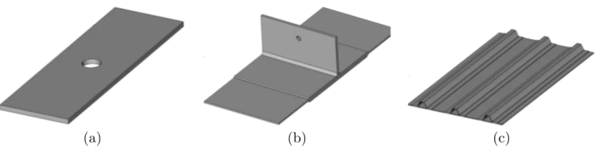
The strategy presented above is now illustrated on some CAD parts. The idealized CAD parts (see figure 4) were provided by EADS IW, and are representative of substructures that are commonly found in the aerospace industry. The first one (figure 4(a)) represents a plate containing a hole at its centre, the second one (figure 4(b)) a glued junction and the third one (figure 4(c)) a stiffened panel. In particular, we will study the influence of the number of levels and the size of level 0 elements. Note that in all these examples, we will consider level 0 elements whose size is close to the thickness of the part (typically close to one half on the thickness): The use of such mesh density will be justified in section 4.
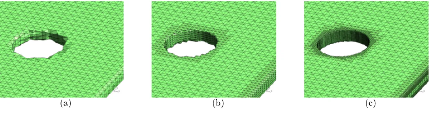
2.2.1. Perforated plate
The geometry of the plate is 30 × 90 × 2mm. Two types of level 0 meshes are considered: (i) Lx = Ly = Lz = 1.2mm and Lx = Ly = Lz = 0.6mm. These meshes are relatively coarse with respect to the thickness of the plate. The influence of the number of sub-grids levels is studied in figures 5 et 6 for mesh Lx = Ly = Lz = 1.2mm and 7 and 8 for mesh Lx = Ly = Lz = 0.6mm. In these figures, one can see the number of nodes, elements and the computational time required to create the mesh and the level set (on a Quad-Core AMD Opteron Processor 2376, with only one core used). The influence of the refinement near the edges of the model is clearly visible in figures 6 and 8. One can also see that the processing time for a very accurate geometrical accuracy (292100 elements) took only 10 seconds. The error in the volume of the part is given in table 1: it can be seen that the initial volume error is decreased by about 25% when increasing the number of sub-grids.
2 ep
a)
b)
c)
d)
e)
f)
g)
h)
i)
j)
Figure 3: Illustration of the algorithm for constructing the level set: a) Initial geometry; b) face points cloud; c) enlargement of the bounding-box; d) activation of the cells containing “surface points”; e) activations of cells sufficiently close to the surface; f) level 0 mesh; g) activation of level > 0 cells (in red, invalid son cells); h) Level-Set mesh; i) computation of the Level-Set at the nodes of the mesh; j) final mesh + Level-Set (after cancelling cells out of the domain)
(a) (b) (c)
Figure 4: Three structures of interest: (a) perforated plate; (b) glued junction; (c) stiffened panel
(a) (b) (c)
Figure 5: Perforated plate: mesh, Lx= Ly= Lz= 1.2mm. (a), (b) and (c): 0, 1, 2 sub-grids levels. (a) 6200 nodes 23500 elements (0.561s); (b) 13000 nodes 49700 elements (0.885s); (c) 27630 nodes 97768 elements (1.553s)
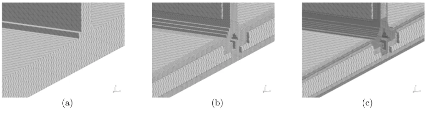
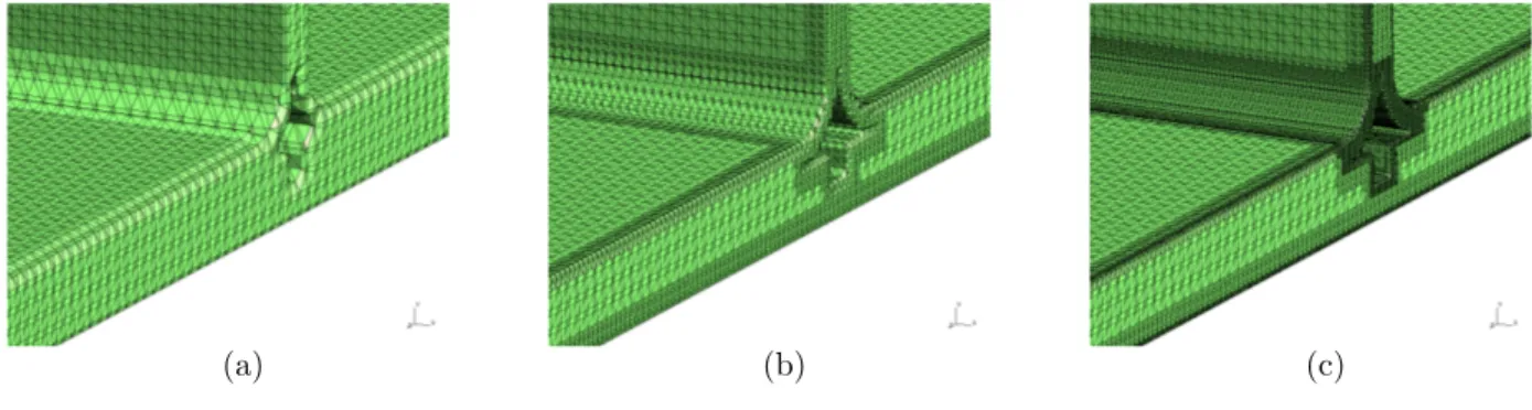
2.2.2. Glued junction
Consider now the glued junction depicted in figure 4(b). The geometry of the part is now close to panel structures that can be found in the aerospace industry. Moreover, it involves different thickness and sharp edges. The size of the bounding-box of the part is 500 × 272 × 1200mm, and the maximum and minimum thickness are respectively 30 and 10mm. Level 0 mesh is composed of Lx = Ly = Lz = 6mm elements (which is quite coarse, greater than one half of the minimum thickness), see figure 9. The influence of the addition of new levels is clearly visible in figure 10: it enables to obtain a good geometrical approximation with a local addition of elements. Looking at the error on the volume of the domain (Table 2), one can see that it remains very small (less than 1%) in all cases although the geometrical description of the sharp features can be quite poor. Concerning the computational time, level sets on extremely fine meshes (typically 1.5 millions of elements) can be generated in less that 2 minutes.
(a) (b) (c)
Figure 6: Perforated plate: iso-zero, Lx = Ly= Lz = 1.2mm. From left to right 0, 1, 2 sub-grids levels. (a) 6200 nodes 23500 elements (0.561s); (b) 13000 nodes 49700 elements (0.885s); (c) 27630 nodes 97768 elements (1.553s)
(a) (b) (c)
Figure 7: Perforated plate: mesh, Lx= Ly= Lz= 0.6mm. From left to right 0, 1, 2 sub-grids levels. (a) 38400 nodes 179000 elements (6.747s); (b) 53300 nodes 227200 elements (7.739s); (c) 76500 nodes 292100 elements (10.095s).
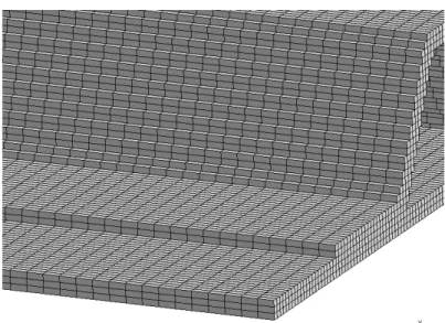
2.2.3. Stiffened panel
Finally, consider the stiffened panel depicted in figure 4(c). The geometry of the part is also close to structures that can be found in the aerospace industry. The size of the bounding-box of the part is 38.7 × 600 × 1000mm, and the maximum and minimum thickness are respectively 6 and 2.94mm. Level 0 mesh is composed of Lx = Ly = Lz = 1.5mm elements (about one half of the minimum thickness). By imposing this size for the elements, one can see in figure 11 that only one level of grid ensures a good geometrical approximation (see figure 12). In this example, it is also possible to keep the same geometrical accuracy by taking into account the particular geometry of the part: it is extruded along z direction. Thus, it is appealing to choose bigger elements in this direction: a Lx= Ly = 1.5mm, Lz= 4mm level 0 grid is considered. The resulting mesh is depicted
(a) (b) (c)
Figure 8: Perforated plate: iso-zero, Lx = Ly = Lz = 0.6mm. From left to right 0, 1, 2 sub-grids levels. (a) 38400 nodes 179000 elements (6.747s); (b) 53300 nodes 227200 elements (7.739s); (c) 76500 nodes 292100 elements (10.095s).
(a) (b) (c)
Figure 9: Glued junction: meshes, Lx = Ly= Lz = 6mm. From left to right 0, 1, 2 sub-grids levels. (a) 112000 nodes 538000 elements (99s); (b) 187500 nodes 851000 elements (111s); (c) 399000 nodes 1 745 980 elements (160s)
in figure 13, and the corresponding Level-Set in figure 14. The size of the mesh is drastically reduced without sacrificing the geometrical description. Note however that finding preferential directions can be difficult in practice, as these directions are usually associated to local axes of the part: these axes are usually not aligned with the global axis of the computational domain. The processing time is longer in this example (6140s), because of the size of the point cloud (61, 244, 302 points): this is linked to the thickness that is extremely small with respect to the size of the structure.
To conclude this section, we have proposed a systematic and pragmatic approach for the con-struction of the implicit representation of complex CAD structures. The computational efficiency of the approach was demonstrated. One can note that such a strategy can easily be parallelized in order to further improve its performances (the faces of the model and the nodes of the cloud can be
(a) (b) (c)
Figure 10: Glued junction: iso-zero, Lx= Ly = Lz = 6mm. From left to right 0, 1, 2 sub-grids levels. (a) 112000 nodes 538000 elements (99s); (b) 187500 nodes 851000 elements (111s); (c) 399000 nodes 1 745 980 elements (160s)
Figure 11: Stiffened panel: mesh (Lx= Ly= Lz= 1.5mm), 4 492 189 nodes 8 400 768 elements, 6140s
scattered on different processes). Moreover, note that the strategy can also be applied to massive parts, although a loss of efficiency may occur due to the introduction of a large number of cells out of the part (as the “thickness” parameter is large in this case).
Figure 12: Stiffened panel: level set (Lx= Ly= Lz= 1.5mm), 4 492 189 nodes 8 400 768 elements, 6140s
Algorithm 1: Computation of the Level-Set. Step i) are referring to Figure 3.
Input: CAD definition, Element size (Level 0) Lx, Ly, Lz, maximal thickness Rmax, number of levels Levels
Deducted parameters: resolution = min(Lx, Ly, Lz) and Rtube= 2 max(Lx, Ly, Lz). Step a) Create the STL discretization of the part.
Step b)
foreach Face f do
Based on the STL discretization of the geometry, create a cloud of points on the part’s surface, such as the maximum distance between every points is smaller than resolution. end
if Levels > 1 then foreach Edge e do
Create a cloud of points on the part’s edges, such as the maximum distance between every points is smaller than resolution.
end end Step c)
Compute the bounding-box of the cloud of nodes Enlarge the bounding-box
Compute Nx, Ny et Nz (number of elements along x, y and z) thanks to the knowledge of Lx, Ly, Lzand the bounding-box
Create a regular Nx× Ny× Nz grid of cubic elements Step d), e), f )
foreach Point p on the faces point cloud do
Activate level 0 cells containing p or sufficiently close to p (max distance ±Rmax along x, y et z)
end
Step g) for Level CurrentLevel=1 to Levels do foreach Point p on the edges point cloud do
Activate level CurrentLevel cells containing p or sufficiently close to p (max distance ±Rtube/2Levels−CurrentLevel−1 along x, y et z)
end end
Step h) Cancel invalid son cells (see Algorithm 2) Step i)
Computation of the level set : foreach CAD Surface f do
foreach STL face fstldo
Compute the distance from all active nodes to face fstl end
end
Step j) Cancel cells out of the domain (positive Level-Set for all nodes). Step k) Find orphan (hanging) nodes
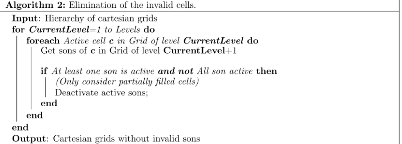
Algorithm 2: Elimination of the invalid cells. Input: Hierarchy of cartesian grids
for CurrentLevel=1 to Levels do
foreach Active cell c in Grid of level CurrentLevel do Get sons of c in Grid of level CurrentLevel+1
if At least one son is active and not All son active then (Only consider partially filled cells)
Deactivate active sons; end
end end
Output: Cartesian grids without invalid sons
Level 0 elements Levels Volume error (%) Lx= Ly = Lz= 1.2mm 0 10.38 Lx= Ly = Lz= 1.2mm 1 7.48 Lx= Ly = Lz= 1.2mm 2 6.92 Lx= Ly = Lz= 0.6mm 0 2.69 Lx= Ly = Lz= 0.6mm 1 2.1 Lx= Ly = Lz= 0.6mm 2 2.04
Table 1: Volume error, perforated plate
Level 0 elements Levels Volume error (%) Lx= Ly = Lz= 6mm 0 0.73 Lx= Ly = Lz= 6mm 1 0.689 Lx= Ly = Lz= 6mm 2 0.526
3. The eXtended Finite Element Method
The X-FEM is an extension of the finite element method (FEM) that was developed from the need to improve the FEM approach for problems with complex and evolving geometries. In contrast to classical finite elements, the X-FEM does not require the mesh to conform the geometry [21, 22]. Instead, one can consider a regular mesh that defines the domain of interest without describing geometrical features such as cracks, inclusions or free surfaces. Then, the approximation is enriched by means of suitable functions to take into account these features. More precisely, the X-FEM approximation of the displacement field, u, over an element is given by:
u(x)|Ωe = n X α=1 Nα uα+ ne X β=1 aαβ ϕβ(x) (1)
where the approximation can be divided into a classical one that depends only on the shape functions Nα(x) and classical degrees of freedom (dofs in the following) uα, and an enriched one that depends on enrichment functions ϕβ(x) and enriched dofs aαβ. Those functions allow to take the non-conforming geometrical features into account in the approximation. The additional degrees of freedom are only added to the nodes whose support is split by the interface, which means that typically only a few of them are added. In the case of free surfaces, as in this contribution, no enrichment has to be considered: only the matter part of the domain is considered when integrating the weak form, and no enriched dofs are introduced [21]. Because of the non-conforming geometry, the integration process is conducted using a modified Gauss quadrature scheme, as described in [9]. The number of integration points over each subdomain is chosen so that the integration is ’exact’. In the present contribution, quadratic approximations will be considered in order to model the mechanical fields that occurs in plate structures with a minimum number of elements. As presented in the previous section, the geometry on the structure is defined implicitly on nested meshes. This type of mesh produces so-called hanging nodes that have to be treated properly in order to ensure the conformity of the approximation. Some strategies have been proposed in order to overcome this issue [23, 24, 25]: In the present contribution, the approach proposed by Legrain et al. [24] will be considered. It is now necessary to characterize the approximation that is used in the approach. Numerous contributions studied the simulation of thin structures with finite elements. If low order elements are used, their bad approximation of the physical behaviour of such structures leads to locking phenomena. This phenomenon can appear for both 3D and 2D
modelling of plates and shells. In both cases dedicated formulations has to be taken into account. If the plate is idealized by its mid-plane, a 2D model can be considered. However, mixed formulations [26, 27, 28, 29, 30] or reduced integration approaches [5, 6, 7] must be used in order to avoid locking issues. Mixed formulations are based on the introduction of rotational degrees of freedom in the approximation. In contrast, under-integrated elements allows to use a displacement based formulation. Unfortunately, selective reduced integration causes zero energy modes that have to be eliminated [31]. Moreover, the material law have to be modified for these models, which can be difficult for non-linear constitutive laws. In addition, the transition between such bidimensional areas to massive one can lead to stress concentrations if a rigid link is prescribed between the two models. Richer approaches have thus to be considered, but they lead to a computational overhead, especially for complex structures. An alternative consists in the use of three-dimensional elements. It is known that displacement-based low order elements are not able to represent the behaviour of slender structures, as locking occurs for both thick and thin plates. This is why so called solid-shell elements have been proposed in the literature. Two main approaches arise: the first one is based on the use of low order finite elements whose behaviour has to be enhanced in order to represent the kinematics of shells [32, 33, 34]. The numerical efficiency of those elements is usually achieved using selective integration approaches [35, 36, 37, 31], which can also lead to hourglass modes. The last possibility was advocated recently by Duster et al. [2]: The authors proposed to use very large conforming elements, but with a high polynomial order. This approach was shown not to be sensitive to locking issues if sufficiently high order polynomial basis functions are used (typically order 6 to 8). The authors applied this strategy to both Reisner-Mindlin plates (using 2D p-FEM) [38] and three-dimensional curved structures (using 3D p-FEM) [2].
An intermediate possibility for the use of solid elements was proposed by Lee and Xu [39, 1] for applications in offshore structures where both thin and thick plates coexist. Performing a cost study for quadratic and cubic approximations, the authors deduced that quadratic elements were a good compromise between computational cost and accuracy [15, 16]. Moreover, they showed that it was more efficient to refine the computational mesh first in the plane of the plate then in the thickness. This is the strategy that we will pursue here. A non-conforming 3D quadratic mesh will be considered for both approximation and geometrical representation. In order to be able to describe implicitly the typical geometry of thin structures with Level-Sets, the size of the mesh must be close to the minimal thickness of the part. This geometrical requirement guided the geometrical
examples presented in the last section. The objective of the next examples is to assess this strategy on some model problems.
4. Verifications
4.1. Thin structure
Consider a clamped square plate shown in figure 15. The length of the plate is 6mm and its thickness h is set to 0.023438mm so that the Kircchhoff theory can be considered. If the external load is denoted f , the deflection at the centre of the plate can be approximated by the following expression:
uc= 0.00126f L 4
D (2)
Where D is called ’plate stiffness’:
D = Eh 3
12(1 − ν2) (3)
With E and ν respectively the Young’s modulus and Poisson’s ratio of the material. If we select E = 1.MPa and ν = 0.3, then uc= 1.3850 106mm.
X Y
Z
Figure 15: Clamped plate subjected to a uniform pressure
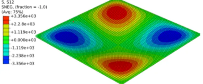
First, consider the case where the geometry is exact (the Level-Set is taken analytically), so that only the approximation induces errors. In addition, the mesh is aligned with the plate. A reference shell computation (18726 dofs) involving 60 × 60 abaqus S4R5 1 elements is considered for comparison with the analytical solution and to define a reference in-plane shear stress field. The discrepancy between this shell solution and the analytical one is 0.433% (uc= 1.391 106mm in
14-node thin shell, reduced integration with hourglass control, using five degrees of freedom per node (two rotations and three displacements)
this case). The amplitude of the corresponding reference in-plane shear stress is ±3356MPa (see figure 16).
Figure 16: Clamped plate subjected to a uniform pressure: In-plane shear stress.
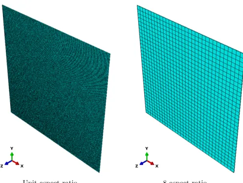
Next, three solid modelizations with one element in the thickness are considered: (i) unit as-pect ratio (0.023438 × 0.023438 × 0.023438mm elements); (ii) asas-pect ratio = 8 (0.1875 × 0.1875 × 0.023438mm elements) and (iii) aspect ratio = 16 (0.375 × 0.375 × 0.023438mm elements) (see figure 17 and 18).
The results are summarized in table 3: It can be seen that the mesh with a unit aspect ratio induces a 0.31% error on the deflection and 0.02% for the in-plane shear stress. Increasing the aspect ratio to 8 increases moderately the errors, while with a 16 aspect ratio begins to exhibit large errors. If tetrahedral elements are considered, then the influence of the aspect ratio is much more pronounced. This illustrates the fact that tetrahedral elements are more sensitive to distortions than hexahedral elements.
For X-FEM and using similar elements (see for example figure 19), the error on the deflection is consistent with the finite element case (2.16%), while the error on the shear stress is lower than the finite element counterpart (0.13%). The difference stems from the fact that two half elements are used in the thickness of the plate, so that the approximation space is not exactly the same as the finite element one. However, this validates the fact that using the X-FEM do not modify the performance of the underlying finite element approach. Note also that, as explained in [1], the large increase of the error in the case of a 16 aspect ratio with tetrahedrons is due to an insufficient discretization in the plane of the plate.
This small verification shows that thin structures can be accurately simulated with X-FEM using low order solid elements, provided that a sufficient number of elements are generated in the plane. This minimum number of elements is obtained naturally within the proposed strategy, as
Unit aspect ratio 8 aspect ratio
Figure 17: Clamped plate subjected to a uniform pressure: solid meshes
the two surfaces of the plate cannot pass through a unique element.
4.2. Thick structure
The same tests can be applied on a thick plate whose dimensions are 6 × 6 × 0.3mm (aspect ratio=20). The results obtained with different discretizations are presented in table 4 and are compared to a reference solution which was computed using 120 × 120 abaqus S8R6 2 elements (deflection 6.957 102mm, σM ax
12 = 19.993MPa). In these examples, variations of both aspect ratio and element size were considered. From these results, one can see that a good accuracy can be obtained using solid elements of size comparable to the thickness of the plate (less than one percent of discrepancy with respect to the reference solution). Obviously, using smaller elements improves the accuracy. Using flattened elements increases the error above to about two percent, but this also stems from the fact that the number of dofs has dropped. As in the thin case, tetrahedral elements
28 nodes doubly curved thick shell with reduced integration, using six degrees of freedom per node (three rotations and three displacements).
16 aspect ratio 16 aspect ratio (tetrahedral elements)
Figure 18: Clamped plate subjected to a uniform pressure: solid meshes
are shown to be a bit more sensitive to distortions.
In the X-FEM case (see figure 20 for a typical mesh), the conclusions are similar than in the case of thin plates (see Table 6): the use of the X-FEM do not modify the behaviour of the elements. Nevertheless, some discrepancies can appear, due to the fact that the approximation space obtained after cutting the elements is different from the one obtained with a conforming mesh.
4.3. Application of the proposed approach
Now, the complete strategy proposed above is applied with the example of the clamped plate. Both thick and thin cases are considered. In the two cases, a CAD file representing the plate is defined. Then, this file is taken as an input of the mesh-generation routine. The boundary conditions are imposed by means of a penalty method. Note that Lagrange multiplier method [40, 41] or Nitsche’s method [42] could be equally used. As the process tends to smooth geometrical angles, an approximation is introduced in the boundary conditions. In practice, the elements of the iso-zero are selected for the boundary conditions when the distance of their centroid to a given plane
Figure 19: Clamped plate subjected to a uniform pressure: typical X-FEM mesh (aspect ratio: 16).
Aspect ratio Type of elements Deflection error (%) In-plane shear stress error (%)
1 Hex 0.31 0.02 8 Hex 1.16 0.06 16 Hex 3.57 0.75 1 Tet 0.31 1.05 8 Tet 1.73 1.52 16 Tet 19.13 31.56 8 Tet X-FEM 2.16 0.13 16 Tet X-FEM 18.41 8.9 16 Tet (2/thickness) 22.6 13.5
Table 3: Influence of mesh density and aspect ratio on the error (thin plate)
is lower than a prescribed threshold. The higher this threshold, the higher the number of elements whose displacement is prescribed, and thus the stiffer the behaviour of the plate in this particular case. This is illustrated in figure 21 where the actual boundaries of the plate are compared with the CAD one. The deflection results are given in table 5. One can see the influence of the selection of the boundaries: smaller boundaries results in a higher deflection at the centre of the plate. Depending on this parameter, the errors in deflection and shear stress vary respectively from 1.28% to 2.16% and 0.86% to 1.1%. Moreover, it can be seen that a good accuracy can be obtained in this case, with elements whose aspect ratio is moderate. The case of the thick plate (thickness 0.3mm) is now considered: The base mesh is composed of a 0.15 × 0.15 × 0.15mm quadratic elements level 0 mesh. In order to represent accurately the boundaries of the domain, 1, 2 and 3 levels are added: Figure 22 depicts the influence of adding multiple levels to the initial mesh. The deflection and shear stress errors are given in table 6. One can see that although the deflection error is decreasing, the shear error do not decrease monotonously upon mesh refinement. This is due to the reference that is used:
Figure 20: Clamped plate subjected to a uniform pressure: Typical X-FEM mesh (aspect ratio: 1)
Aspect ratio Elts/thickness Type of elements Deflec. error (%) In-plane shear stress error (%)
1 1 Hex 4.07 0.665 1 2 Hex 0.934 0.015 1 1 Tet 1.25 0.665 1 2 Tet 0.747 0.185 2 1 Hex 5.203 1.986 4 2 Hex 3.177 2.336 2 1 Tet 6.67 4.767 4 2 Tet 4.657 3.216 1 0.8 Tet X-FEM 3.222 6.033 1 1.6 Tet X-FEM 1.349 1.053 2 1.6 Tet X-FEM 2.651 2.746 4 3.2 Tet X-FEM 2.173 2.891
Table 4: Errors depending on mesh density and aspect ratio (thick plate)
it was obtained using shell elements that may not represent the three dimensional behaviour of the plate. An overkill FEM solution is computed in order to build a reference (0.06 × 0.06 × 0.06mm quadratic elements). The figures inside the brackets show the errors (in both deflection and stress) with respect to this new reference: It can be seen now that the error converges to zero when the number of levels increase, which is consistent.
Finally, we still consider the same example, but now the plate is rotated by an angle of 60◦ in the xy plane in order to study the influence of the orientation of the part with respect to the mesh. 1, 2, 3 and 4 levels are considered, level 0 mesh being composed of 0.15 × 0.15 × 0.15mm quadratic elements. The corresponding meshes and boundaries are depicted in figure 23, and the improvement on the geometry is clearly visible. Deflection errors are presented in table 7 (stress
errors are not depicted, as the plate is not oriented along x and y axis). Like in the previous example, the improvement in term of error is clear when increasing the number of mesh levels. It is also clear that the rotation of the plate almost did not modify the error level (with a monotonous decrease of the error with respect to the overkill FEM solution).
X Y Z X Y Z (a) (b)
Figure 21: Influence of the threshold used to select the boundaries. (a) Large threshold; (b) Small threshold
Aspect ratio Elts/thickness Boundary Deflec. error (%) In-plane shear stress error (%)
6.25 0.293 Small 1.2830 1.1040
6.25 0.293 Large 2.15740 0.86204
Table 5: Influence of mesh density and aspect ratio (thin plate) on the error, using the proposed approach. The two rows show the influence of the selection of the boundaries.
Asp. ratio Elts/thick. Lev. Deflec. err. (%) [/FEM] Shear err. (%) [/FEM] 1 2 1 8.857 [8.3568] 0.5247 [0.1481] 1 2 2 2.230 [1.6929] 1.2409 [0.9531] 1 2 3 0.0985 [0.45021] 1.2079 [0.9202]
Table 6: Influence of mesh density and aspect ratio (thick plate) on the error, using the proposed approach. Influence of the number of sub-grids.
X Y Z X Y Z 1 level 2 levels X Y Z 3 levels
Figure 22: Influence of the number of levels on the representation of the boundaries.
Aspect ratio Elts/thickness Levels Deflec. error (%) Deflec. error /FEM(%)
1 2 1 5.741 5.2233
1 2 2 2.644 2.1096
1 2 3 1.249 0.9744
1 2 4 1.249 0.7069
Table 7: Influence of mesh density and aspect ratio (thick plate) on the error, using the proposed approach. Influence of the number of sub-grids for the rotated case.
X Y Z X Y Z 1 level 2 levels X Y Z X Y Z 3 level 4 levels
5. Numerical examples
The proposed approach is now illustrated on some idealized CAD parts provided by EADS IW. These structures are representative of substructures that are commonly found in the aerospace industry. Of increasing complexity, the objective here is to illustrate the potential of the approach.
5.1. Drilled plate 5.1.1. Qualitative results
We are interested in the simulation of the behaviour of the drilled plate shown in figure 4(a). The boundary conditions that are considered are depicted in figure 24: they represent combined traction and bending loadings by means of a prescribed displacement. Three meshes are considered: (i) a regular Lx= Ly= Lz= 0.6mm elements mesh, (ii) a regular Lx= Ly = Lz = 1.2mm elements mesh with two grid levels and (ii) a regular Lx= Ly = Lz= 1.2mm elements mesh with three grid levels. These meshes are shown in figures 7(a) and 5(b) and (c) respectively.
X Y Z
Figure 24: Geometry and boundary conditions.
The results are presented in figures 25 , 26 and 27 for the proposed cases. One can see that despite of the fact that the level 0 mesh in figures 26 and 27 is twice coarser than the mesh in figure 25, the mechanical fields (both displacement and Von-Mises norm of the stress) are similar and extremely smooth. Adding mesh levels allows similar or better geometrical accuracy depending on the number of levels involved, but with a smaller amount of dofs than homogeneous refinement.
5.1.2. Quantitative results
In order to deal with quantitative results, the error in the strain energy is computed from the previous results. The reference energy is obtained by means of an overkill conforming finite element
(a) (b)
(c) (d)
Figure 25: Drilled plate in traction and bending (Lx= Ly= Lz= 0.6mm elements, one mesh level) : (a), (b), (c) : displacement ; (d) stress (Von Mises norm)
solution with a fourth order polynomial approximation (594 060 dofs). The results are summarized in Table 8. In particular, it can be seen that the use of multiple mesh levels greatly improves the accuracy and the efficiency of the approach: the coarse mesh Lx = Ly = Lz = 1.2mm with two levels gives a lower error and fewer dofs than the fine mesh (Lx = Ly = Lz = 0.6mm) with only one level.
The convergence of the approach is finally assessed by means of homogeneous mesh refinement. Meshes of size Lx = Ly = Lz = 0.8, 0.4, 0.3 and 0.25mm are considered, and the error in the strain energy is computed with respect to the reference solution. The results are presented in figure 28. It can be seen that the convergence rate is close to the optimal one (i.e. 2 as a quadratic approximation is used). Theoretically, the convergence rate should be bounded by O(h3/2) (see
(a) (b)
(c) (d)
Figure 26: Drilled plate in traction and bending (Lx= Ly= Lz= 1.2mm elements, two mesh levels): (a), (b), (c): displacement ; (d): stress (Von Mises norm)
[43, p 119] and [44]). However, it was shown in [45] that optimal convergence could nevertheless be obtained in practice, depending on the problem (which seems to be the case here). The influence of the integration is now assessed: rather than partitioning the elements along the iso-zero of the Level-Set, a classical integration rule is considered. In order to be able to converge, the number of integration points is increased in the elements that are cut by the interface: a 72 points degenerated quadrangle integration rule is considered in this case: the convergence of this approach is depicted in figure 28: it can be seen that a loss of accuracy can occur depending on the mesh density and most likely on the geometry of the problem. Moreover, increasing the number of integration points on such fine meshes has a huge impact on the computational time. Note also that if the number of integration points is insufficient, then the stiffness matrix can become singular. This minimum
(c) (d)
Figure 27: Drilled plate in traction and bending (Lx = Ly = Lz = 1.2mm elements, three mesh levels): (a), (b): displacement ; (c), (d): stress (Von Mises norm)
number of points depend on both mesh and geometry. The advantage of such an approach stems from the fact that the burden of creating the sub-elements is avoided. A better alternative would consist in the use of this incompatible integration strategy together with the exact CAD description of the geometry (like with the Finite Cell [2]).
5.2. Glued junction
The case of the glued junction is now considered. Here, only one part of the junction is presented in order to run on a personal computer. The part is subjected to a uniaxial traction along z by means of a prescribed displacement (100mm along z) on face z+ (cf figure 29) and zero dirichlet B.C. on face z−.
Mesh Levels dofs Error (%) Lx= Ly = Lz= 0.6mm 1 662106 0.579 Lx= Ly = Lz= 1.2mm 2 357828 0.495 Lx= Ly = Lz= 1.2mm 3 709368 0.159
Table 8: Strain energy error, drilled plate
10-1 100 h 10-4 10-3 10-2 10-1
Strain energy error
2 X-FEM - Quadratic
X-FEM - Quadratic incomp. integ.
Figure 28: h-convergence of the proposed approach. It can be seen that optimal rate is obtained when the integration is done properly. On the contrary, incompatible integration can lead to a loss of convergence if the number of integration points is not severely increased.
A two level mesh with Lx = Ly = Lz = 6mm for level 0 elements is considered. The mesh is composed of 249 816 quadratic tetrahedra (1 051 404 dofs). Thanks to the use of solid elements, the junction between the different parts is taken into account without any hypothesis on the geometry of the different sub-parts. The displacement and stress fields are displayed in figure 30. Stress concentrations are captured by the solution at the centre of the junction. These informations could not be obtained using a plate model.
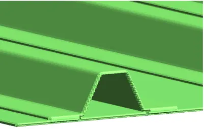
5.3. Stiffened plate
Finally, the stiffened plate presented in section 2.2 is considered. Like in the previous example, only one part of the plate is considered in order to allow its treatment on a personal computer. The corresponding geometry is presented in figure 31. Like in section 2.2, the Level-Set is computed on a mesh composed of only one level of elements (1.5 × 1.5 × 4mm elements), as the geometrical
X Y Z
Figure 29: Boundary conditions for the junction
accuracy is sufficient. The part is then subjected to a bending loading by applying the boundary conditions depicted in figure 31. The size of the corresponding model is 2 452 461dofs, and the results are presented in figure 32 for both deformed configuration and stress.
Displacement Stress
Stress (Zoom)
Figure 30: Glued junction: results for a two levels mesh (Level 0: Lx= Ly= Lz= 6mm)
X Y Z
Displacement
Displacement
Stress
Stress b
6. Conclusion
In this contribution, an integrated approach was proposed in order to simulate the behaviour of aerospace CAD-based thin structures. The proposed strategy relies on the combined use of the eXtended Finite Element method and the Level-Set approach. As the method is non-conforming, there is no need to explicitly mesh the volume of the domain of interest: the computation is done on a regular grid of elements which also supports the geometrical description (thanks to the Level-Set approach). An algorithm was proposed in order to convert complex CAD parts into a Level-Set and a mesh support. The use of a nested set of grids makes possible the description of sharp edges with Level-Sets. Although less accurate than the algorithm proposed by Moumnassi et al. [17], our implementation is tolerant to damaged CAD geometries (with overlap or holes). Note however that the parallelization of the algorithm would improve its efficiency. The use of solid elements was also proposed, as it avoids the construction of mid-plane surfaces, and also makes natural the modelization of junctions between thin and massive parts. The approach was applied to some academic examples, then to representative CAD parts. It was shown that a very good accuracy could be obtained. The efficiency of the approach could be improved by means of the parallelization of the Level-Set computation. Current work on this topic focus now on the use of higher order approximations together with the separation between geometry and mechanical approximation using the approaches developed in [46, 47] (see the illustrative example shown below), or [48]. It could also be applied to geometries defined by means of surface scanners as a tool for reverse engineering.
7. Outlook
The improvement of the approach proposed in the conclusion is illustrated here. In order to save degrees of freedom with a fixed geometrical accuracy, an approach derived from [47] is considered. The geometry is represented on the fine grid depicted in figure 33, and the approximation is defined on the mesh shown in figure 34. The problem is subjected to the same BCs as in section 5.1. A P6 approximation is considered, leading to 106 953 dofs (which is far less than in section 5.1). The resulting stress and displacement fields are given in figure 35 (note that the stress field was not smoothed at all). The corresponding error in the strain energy is 0.007% which couldn’t be attained using the approach advocated in this paper, unless a million of dofs are used.
Figure 33: Geometrical grid and iso-surface
REFERENCES
[1] C.K. Lee and Q.X. Xu. Automatic adaptive fe analysis of thin-walled structures using 3d solid elements. International Journal for Numerical Methods in Engineering, 76:183–229, 2008.
[2] A. Duster, D. Scholz, and E. Rank. pq-adaptive solid finite elements for three-dimensional plates and shells. Comput. Methods Appl. Mech. Engrg., 197:143–254, 2007.
[3] E. Wilson, R. Taylor, W. Doherty, and J. Ghaboussi. Incompatible displacement models, volume numerical and computer models in structural mechanics, chapter numerical and computer models in structural mechanics, pages 43–57. Academic Press, New York, 1973.
[4] RL. Taylor, PJ. Beresford, and EL. Wilson. A nonconforming element for stress analysis. International Journal for Numerical Methods in Engineering, 10(6):1211–1219, 1976.
[5] O.C. Zienkiewicz, R.L. Taylor, and J.M. Too. Reduced integration technique in general analysis of plates and shells. International Journal for Numerical Methods in Engineering, 3:275–290, 1971.
Figure 34: Approximation mesh and iso-surface
Figure 35: Displacement and stress fields. Note that the stress field was not smoothed at all.
[6] T.J.R. Hughes, M. Cohen, and M. Haroun. Reduced and selective integration techniques in finite element analysis of plates. Nuclear Engineering Design, 46:203–222, 1978.
[7] T.J.R. Hughes. Generalization of selective integration procedures to anisotropic and nonlinear media. International Journal for Numerical Methods in Engineering, 15:1413–1418, 1980.
[8] H. Ben-Dhia and G. Rateau. The arlequin method as a flexible engineering design tool. Inter-national Journal for Numerical Methods in Engineering, 62:1442–1462, 2005.
[9] N. Mo¨es, J. Dolbow, and T. Belytschko. A finite element method for crack growth without remeshing. International Journal for Numerical Methods in Engineering, 46:131–150, 1999.
[10] S. Osher and J.A. Sethian. Fronts propagations with curvature dependent speed: Algorithms based on Hamilton-Jacobi formulations. Journal of Computational Physics, 79:12–49, 1988.
[11] J.M. Melenk and I. Babuˇska. The partition of unity finite element method : Basic theory and applications. Comp. Meth. in Applied Mech. and Engrg., 139:289–314, 1996.
[12] Thomas-Peter Fries and Ted Belytschko. The extended/generalized finite element method: An overview of the method and its applications. International Journal for Numerical Methods in Engineering, 84(3):253–304, 2010.
[13] Abdelaziz Yazid, Nabbou Abdelkader, and Hamouine Abdelmadjid. A state-of-the-art re-view of the X-FEM for computational fracture mechanics. Applied Mathematical Modelling, 33(12):4269–4282, 2009.
[14] V.K. Saul`ev. On the solution of some boundary value problems on high performance computers by fictitious domain method. Siberian Math. J., 4:912–925, 1963.
[15] C.K. Lee and S.H. Lo. Automatic adaptive 3-d finite element refinement using different-order tetrahedral elements. International Journal for Numerical Methods in Engineering, 40:2195– 2226, 1997.
[16] C.K. Lee and S.H. Lo. Automatic adaptive refinement finite element procedure for 3d stress analysis. Finite elements in analysis and design, 25:135–136, 1997.
[17] Mohammed Moumnassi, Salim Belouettar, ´Eric B´echet, St´ephane P.A. Bordas, Didier Quoirin, and Michel Potier-Ferry. Finite element analysis on implicitly defined domains: An accurate representation based on arbitrary parametric surfaces. Computer Methods in Applied Mechan-ics and Engineering, 200(5-8):774–796, 2011.
[18] C. Geuzaine and J.F. Remacle. Gmsh: A 3-d finite element mesh generator with built-in pre-and post-processing facilities. International Journal for Numerical Methods in Engineering, 79:1309–1331, 2009.
[19] Open cascade technology, an environment for 3d modeling. http://www.opencascade.org.
[20] P. Frey and P. George. Mesh Generation: Application to Finite Elements. Hermes Science Publishing Ltd;, 2000.
[21] N. Sukumar, D. L. Chopp, N. Mo¨es, and T. Belytschko. Modeling Holes and Inclusions by Level Sets in the Extended Finite Element Method. Comp. Meth. in Applied Mech. and Engrg., 190:6183–6200, 2001.
[22] T. Belytschko, C. Parimi, N. Mo¨es, S. Usui, and N. Sukumar. Structured extended finite element methods of solids defined by implicit surfaces. International Journal for Numerical Methods in Engineering, 56:609–635, 2003.
[23] A. Tabarraei and N. Sukumar. Extended finite element method on polygonal and quadtree meshes. Computer Methods in Applied Mechanics and Engineering, 197(5):425–438, 2008.
[24] G. Legrain, R. Allais, and P. Cartraud. On the use of the eXtended Finite Element Method with Quatree/Octree meshes. International Journal for Numerical Methods in Engineering, 86(6):717–743, 2011.
[25] T.P. Fries, A. Byfut, A. Alizada, K.W. Cheng, and A. Schr¨oder. Hanging nodes and XFEM. International Journal for Numerical Methods in Engineering, 86:404–430, 2011.
[26] O.C. Zienkiewicz and D. Lefebvre. A robust triangular plate bending element of the Reissner– Mindlin type. International Journal for Numerical Methods in Engineering, 26:1169–1184, 1988.
[27] K.J. Bathe and E.N. Dvorkin. Four-node plate bending element based on Mindlin/Reissner plate theory and a mixed interpolation. International Journal for Numerical Methods in En-gineering, 21:367–383, 1985.
[28] K.J. Bathe and E.N. Dvorkin. Formulation of general shell elements – The use of mixed inter-polation of tensorial components. International Journal for Numerical Methods in Engineering, 22:697–722, 1986.
[29] K.J. Bathe and L.W. Ho. A simple and effective element for analysis of general shell structures. Computers and Structures, 13:673–681, 1981.
[30] J.L. Batoz and M. Ben Tahar. Evaluation of a new thin plate quadrilateral element. Interna-tional Journal for Numerical Methods in Engineering, 18:1655–1678, 1982.
[31] D.P. Flanagan and T. Belytschko. A uniform strain hexahedron and quadrilateral with orthogo-nal hourglass control. Internatioorthogo-nal Jourorthogo-nal for Numerical Methods in Engineering, 17:679–706, 1981.
[32] J.C. Simo and M.S. Rifai. A class of mixed assumed strain methods and the method of incompatible modes. International Journal for Numerical Methods in Engineering, 29:1595– 1638, 1990.
[33] J.C. Simo and F. Armero. Geometrically non-linear enhanced strain mixed methods and the method of incompatible modes. International Journal for Numerical Methods in Engineering, 33:1413–1449, 1992.
[34] J.C. Simo, F. Armero, and R.L. Taylor. Improved versions of assumed enhanced strain trilinear elements for 3d finite deformation problems. Computer Methods in Applied Mechanics and Engineering, 110:359–386, 1993.
[35] O.C. Zienkiewicz, R.L. Taylor, and J.M. Too. Reduced integration technique in general analysis of plates and shells. International Journal for Numerical Methods in Engineering, 3:275–290, 1971.
[36] T.J.R. Hughes. Generalization of selective integration procedures to anisotropic and nonlinear media. International Journal for Numerical Methods in Engineering, 15:1413–1418, 1980.
[37] B.G. Prathap and G.R. Bhashyam. Reduced integration and the shear flexible beam element. International Journal for Numerical Methods in Engineering, 18:195–210, 1982.
[38] E. Rank, A. Duster, V. Nubel, K. Preusch, and O.T. Bruhns. High order finite elements for shells. Comput. Methods Appl. Mech. Engrg, 194:2494–2512, 2005.
[39] C.K. Lee and Q.X. Xu. A new automatic adaptive 3d solid mesh generation scheme for thin-walled structures. International Journal for Numerical Methods in Engineering, 62:1519–1558, 2005.
[40] N. Mo¨es, E. B´echet, and M. Tourbier. Imposing Dirichlet boundary conditions in the ex-tended finite element method. International Journal for Numerical Methods in Engineering, 67(12):1641–1669, 2006.
[41] E. B´echet, N. Mo¨es, and B. Wohlmuth. A stable lagrange multiplier space for the stiff interface conditions within the extended finite element method. International Journal for Numerical Methods in Engineering, 78(8):931–954, 2009.
[42] J. Nitsche. ¨Uber ein Variationprinzip zur l¨osung von Dirichlet-Problem bei Verwendung von Teilr¨aumen, die keinen Randbedingungen unterworfen sind. Abh. Math. Sem. Univ. Hamburg, 36:9–15, 1971.
[43] Pierre Arnaud Raviart and Jean-Marie Thomas. Introduction ´a l’analyse num´erique des ´
equations aux d´eriv´ees partielles. Dunod, Paris, 1998.
[44] G. Legrain, N. Mo¨es, and A. Huerta. Stability of incompressible formulations enriched with X-FEM. Computer Methods in Applied Mechanics and Engineering, 197(21-24):1835–1849, 2008.
[45] Kristell Dr´eau, Nicolas Chevaugeon, and Nicolas Mo¨es. Studied X-FEM enrichment to handle material interfaces with higher order finite element. Computer Methods in Applied Mechanics and Engineering, 199(29-32):1922–1936, 2010.
[46] G. Legrain, N. Chevaugeon, and K. Dr´eau. High order eXtended Finite Element Method and Level Sets: Uncoupling geometry and approximation. In XFEM 2011 : Partition of unity enrichment: Recent developments and applications, 2011.
[47] G. Legrain, N. Chevaugeon, and K. Dr´eau. High order X-FEM and levelsets for complex microstructures: Uncoupling geometry and approximation. Computer Methods in Applied Mechanics and Engineering, 241–244(0):172–189, 2012.
[48] G. Legrain. A NURBS Enhanced eXtended Finite Element Approach for Unfitted CAD Anal-ysis. Computational mechanics, DOI: 10.1007/s00466-013-0854-7, 2013.