A timed extension for AltaRica

HAL Id: inria-00363026

https://hal.inria.fr/inria-00363026

HAL is a multi-disciplinary open access

archive for the deposit and dissemination of sci-entific research documents, whether they are pub-lished or not. The documents may come from teaching and research institutions in France or abroad, or from public or private research centers.

L’archive ouverte pluridisciplinaire HAL, est destinée au dépôt et à la diffusion de documents scientifiques de niveau recherche, publiés ou non, émanant des établissements d’enseignement et de recherche français ou étrangers, des laboratoires publics ou privés.

Franck Cassez, Claire Pagetti, Olivier Roux

To cite this version:

Franck Cassez, Claire Pagetti, Olivier Roux. A timed extension for AltaRica. Fundamenta Informat-icae, Polskie Towarzystwo Matematyczne, 2004, 62 (3–4), pp.291–332. �inria-00363026�

A Timed Extension for AltaRica

Franck Cassez, Claire Pagetti and Olivier Roux

IRCCyN 1 rue de la Noë BP 92101 44321 Nantes Cedex 3 France email: Name.Surname@irccyn.ec-nantes.fr

Abstract. In this paper we present a timed extension of theAltaRicaformalism. Following previous works, we first extend the semantics ofAltaRicawith time and define timed components and timed nodes. Moreover we lift the priority features ofAltaRicato the timed case. We obtain a timed version ofAltaRica, calledTimed AltaRica. Finally we give a translation of a Timed AltaRica

specification into a usual timed automaton. These are the semantic foundations of a high-level hierarchical language for the specification of timed systems.

Keywords: AltaRica, Semantics, Timed Automata

1.

Introduction

Context. The development of complex and safety-critical systems requires the use of formal methods

and tools for system design and specification. In the case of discrete systems the so-called reactive

lan-guages [1, 2, 3, 4] have been used for almost a decade to specify industrial systems. They give a rigourous

and elegant basis for the structured development of reactive systems with the use of composition and

hier-archical specifications for instance. On those specifications such techniques like model-checking can be

applied to check for some properties on the designed systems.

The need for a counterpart specification language in the case of timed specifications arose recently

as timing information can now be dealt with while verifying a system with tools like UPPAAL[5],

CMC[6],KRONOS[7] orHyTech[8]. We give here the theoretical foundations of such a high-level

specification language for timed systems. We extend the AltaRica[9, 10, 11] formalism with timing features.

AltaRicais a high-level specification formalism that allows one to specify constraint automata [9] with the following features:

• a component has its own variables (internal or external), plus some others it can only read (flow

variables) that are shared by the others;

• components can be defined hierarchically and composed together by a general synchronization

mechanism. Such a general component is called a node. One can express broadcast communica-tion, give priority among some transitions, etc.

MoreoverAltaRicahas an unambiguous semantics [11, 10] defined in terms of (interfaced) transition

systems. From this semantic model, it is possible to compile AltaRicato lower level formalisms for

different verification purposes: fault-trees to perform reliability analysis [12], Petri nets, Markov graphs

or finite state automata (that can be analysed with the toolMEC[13, 14, 15, 16] for instance).

Nevertheless one cannot specify real-time constraints inAltaRicaand of course this becomes crucial

when some timing information contributes to the modelling and correctness of the system. Moreover

there is no real high-level specification language for timed and hybrid systems. This makesAltaRica

a good candidate to fill this gap. Once the language has been extended with timing constraints, we can take advantage of the work carried out these last years about timed systems: it is now well-known how to deal with the verification of timed automata [17] and hybrid automata [18, 19] and many efficient tools

are now available [8, 7, 20]. This adds a new feature to theAltaRicatoolbox.

Our Contribution. Our work consists in extending theAltaRicaformalism with real-time constraints

and define a timed version ofAltaRicacalledTimed AltaRica. We thus extend the theoretical

founda-tions ofAltaRica: we enhance the semantic model ofAltaRica, the interfaced transition system (ITS),

into timed interfaced transition system (TITS) and give the semantics ofTimed AltaRicain terms of

TITS. We proceed by shifting all the theoretical results obtained forAltaRica(e.g. interface

bisimula-tion homomorphism, rewriting of a node into a component, . . . ) to the timed case: this is important as it

givesTimed AltaRicagood compositional properties that are needed in practice. Finally we present an

algorithm to compileTimed AltaRicaspecifications into timed automata (which can be then analyzed

withUPPAAL[5]).

Outline of the paper. In the next section, we remind the basics aboutAltaRicaand introduce a running

example: the Train-Gate-Controller example. Section 3 is the core of the paper and presents Timed

AltaRicathe timed extension ofAltaRica. In sections 4 and 5 we respectively give (i) the algorithm for

translatingTimed AltaRicacomponents into timed automata and (ii) an example of the use of priorities

for timed specifications. We conclude by some perspectives in section 6. The proofs of the theorems are given in the appendices (pages 1035– 1042).

2.

An Overview of the

AltaRica

Language

In this section we recall some basics ofAltaRica[10, 11] and give an example of anAltaRica

a critical section. We will use three AltaRicacomponents to model the system and describe how they synchronize.

2.1. Specifying Reactive Systems inAltaRica

A specification inAltaRicais a node. A node is a hierarchical description. It can be built from sub-nodes

and so on. A node that contains no sub-nodes is a component. A node is basically composed of:

• the variables definitions (type, range, . . . ), and events definitions, • the transition relation,

• the initial constraint and global constraint.

1: node TRAIN

2: flow N : [0,1]; // These are the flow variables

3: event approach, in, exit; 4: state etat : [0,2]; n : [0,1]; 5: trans

6: etat=0 |- approach ->

7: etat := 1, n := 1; 8: etat=1 |- in -> etat := 2;

9: etat=2 |- exit -> etat := 0, n := 0; 10: init

11: etat:=0, n:=0; 12: assert

13: N=n; 14: edon

(a) Spec. of the Train inAltaRica

Far Before On approach,n:= 1 in exit,n:= 0 Far ≡ etat= 0 Before ≡ etat_{= 1} On ≡ etat= 2

(b) Spec. of the Train as an Automaton

Figure 1. Specification of a Train

2.1.1. Components

In the example of Fig. 1, we define a component1train to model the behaviour of a train in two equivalent

manners in order to ease the understanding: an AltaRica description (see Fig. 1(a)) and a standard

automaton (see Fig. 1(b)). A train is either Far of the critical section, or Before or On meaning it is

respectively near or inside the critical zone. In the AltaRicaspecification, the variable etat (line 4)

ranging in [0, 2] represents the locations Far, Before, On of the train. The events of the component

TRAIN are approach, in and exit (line 3). We also use a state variable n (line 4) to denote that the train is

in{Before, On}. Initially the component is in configuration etat=0,n=0,N=0 (line 11), written (0, 0, 0)

for short. When a transition occurs the values of the state variables change accordingly as well as the

1

InAltaRicathe keyword node in used for components (nodes with no sub-nodes) as well as for hierarchical nodes; indeed a component is a special case of node with no sub-nodes.

value of the flow variable in order to satisfy the assertion (line 13). For instance, when event approach

occurs in(0, 0, 0) the configuration (1, 1, 1) is reached.

2.1.2. Interfaces

The component’s state variables are not visible from outside of the component. Their scope is thus the component itself just as for usual programming languages. To allow sharing of information and synchronization on variables of other components one can use flow variables. Flow variables can be read by other nodes. The part of the component which is visible by other components is called the interface. It consists in the events of the components and the flow variables.

The flow variableN is in the interface of the node TRAIN (line 2). This means that other nodes can

read it and use the value ofN. The value of the flow variable N is constrained to be equal to n at anytime

(see theassert line 13) and the purpose of N is to make the value of n available outside.

Assume another node for the controller is given by theAltaRicaspecification of Fig. 2(a). A

trans-ition of the form etat = 1 |- approach -> ; (line 9) means that approach does not bring about

any change in the state variables values (but not this is a deadlock!). In the componentCONTROLLER the

purpose of the flow variableN (referred to as CONTROLLER.N from now on) is to count the total number

of trains in the region{Before, On} (if we assume there are many train components). Depending on the

value of the flowCONTROLLER.N the controller will make the gate go up on an exit signal (if the value is

1, line 8) or will leave the gate closed if CONTROLLER.N > 1 (line 7).

The value ofCONTROLLER.N may change on any discrete transition and be assigned any integer as no

assertion constrains this flow in the nodeCONTROLLER. Apart from the events listed in the component’s

events section (line 3), we assume a special discrete event² for synchronization purposes. This event is

enabled in any configuration and does not change the values of variables of typestate. Nevertheless

flow variables can be updated on² transitions with values satisfying the assertion. As the assertion of the

nodeCONTROLLER is implicitely true the variable CONTROLLER.N may be assigned any integer value on

an² transition. This somewhat strange behavior will become clear when we introduce hierarchical nodes

and constraints among flows of different nodes (seeassert line`main−asserton Fig. 3).

As for the nodeGATE (Fig. 2(b)) it consists in receiving orders from the controller (events Go_up and

Go_down) and after a while2to actually go up or down (eventsup and down).

2.1.3. Hierarchy and Synchronization

As emphasized in the introduction, one can describe a system by composing and building new nodes

from sub-nodes. For example we can define a nodeMain (see Fig. 3) specifying the train-gate-controller

with two trains. Indeed nodes can be instantiated and used as templates to build higher-level nodes.

The node of Fig. 3 is composed of four instantiated sub-nodes (t1, t2, g and c, see Fig. 3, lines 2–

5) which interact in two ways: flow coordination and synchronization of events. The synchronization

constraint (after keywordsync, lines 6–14) reads as follows: if a component does not appear in a

syn-chronization vector, it is assumed to do the² action. Note that events up and down are not synchronized

and thus they will be assumed to be synchronized with ² transitions of the other components. Finally

the global assertion, line 15, constrains the flow variables so thatN of the node MAIN is always equal

2

We will see later how this can be made precise using timing constraints to make a timed version of the controller and the gate in Fig. 5.

1: node CONTROLLER 2: flow N : [0,p];

3: event approach, exit, Go_up, Go_down; 4: state etat : [0,2];

5: trans

6: etat=0 |- approach -> etat := 1; 7: etat=0 & N>1 |- exit -> ;

8: etat=0 & N=1 |- exit -> etat := 2; 9: etat = 1 |- approach -> ;

10: etat = 1 |- exit -> ;

11: etat=1 |- Go_down -> etat := 0; 12: etat=2 |- Go_up -> etat := 0; 13: etat=2 |- approach -> etat := 1; 14: init etat := 0, z := 0;

15: edon

(a) The Controller

node GATE

event Go_down, Go_up, down, up;

state etat : [0,3];

trans

etat=0 |- Go_up -> ;

etat=0 |- Go_down -> etat := 1; etat=1 |- Go_down -> ;

etat=1 |- down -> etat := 2; etat=1 |- Go_up -> etat :=3; etat=2 |- Go_down -> ; etat=2 |- Go_up -> etat := 3; etat=3 |- Go_up -> ;

etat=3 |- Go_down -> etat := 1; etat=3 |- up -> etat := 0;

init etat:=0;

edon

(b) The Gate

Figure 2. AltaRicaSpecifications for the Controller and the Gate

to the number of trains on the critical section. A joint move of the components t1,t2,g,c can be

<t1.approach,t2.approach,c.approach> (see line 7) in which case the variable c.N will be

up-dated on the² move of component c to satisfy the assertion of node MAIN i.e. c.N=t1.N+t2.N. This

is why we need to have the possibility to update flow variables on² transitions. Anyway a meaningful

specification should be such that all flow variables are constrained at least in the outermost node. Note

that some constraints could be unsatisfiable: for instance if we addt1.N=2+t2.N to the assert line, this

clearly can not be satisfied and the resulting system has no configuration. It is also possible to constrain

the state space: if we uset1.N=t2.N we impose that the two trains issue approach at the same time and

leave the critical section at the same time (eventexit). This is due to the fact that no configuration with

t1.N not equal to t2.N is satisfiable hence no transition with only one approach event can be fired.

1: node MAIN 2: sub 3: t1,t2 : TRAIN; 4: g : GATE; 5: c : CONTROLLER; 6: sync 7: <t1.approach,t2.approach,c.approach>; 8: <t1.approach,c.approach>; 9: <t2.approach,c.approach>; 10: <t1.exit,t2.exit,c.exit>; 11: <t1.exit,c.exit>; 12: <t2.exit,c.exit>; 13: <g.Go_down,c.Go_down>; 14: <g.Go_up,c.Go_up>; 15: assert c.N=t1.N+t2.N; 16: edon

2.2. Formal Semantics ofAltaRica

The semantics of AltaRica specifications is given by Interfaced Transition Systems. For a detailed

presentation of these notions the reader is referred to [11, 10].

2.2.1. Interfaced Transition Systems

Definition 2.1. (Interfaced Transition system [10])

An interfaced transition system (ITS) is a tupleA = hE, F, S, π, T i with:

1. E = E+∪ {ε} is a finite set of events such that ε 6∈ E+;

2. F is a set of flow values;

3. S is the set of states;

4. π : S → 2F _{associates to each state s in S all the admissible flow values in s. We assume}

∀s ∈ S, π(s) 6= ∅.

5. T ⊆ S × F × E × S is the transition relation and satisfies:

(a) (s, f, e, s0) ∈ T ⇒ f ∈ π(s)

(b) ∀s ∈ S, ∀f ∈ π(s), (s, f, ε, s) ∈ T

A configuration of an ITS is a pair(s, f ) ∈ S × F such that f ∈ π(s). Every tuple (s, f, e, s0) ∈ T

corresponds to the set of transitions((s, f ), e, (s0, f0)) between configurations s.t. f0 ∈ π(s0_).

Remark 2.1. InAltaRica, if a transition(s, f, e, s0) is firable then there exists a configuration (s0, f0)

(as item 4 of Def. 2.1 assumesπ(s) is not empty for s ∈ S). This remark will carry over timed ITS. The

setF may be considered as a set of properties (or observations) associated to the states by the mapping π. Also note that T is a shorthand for the explicit transition relation T0 between configurations with

T0 ⊆ S × F × E × S × F and (s, f, e, s0_{, f}0_{) ∈ T}0 _{⇐⇒ (s, f, e, s}0_{) ∈ T ∧ f}0_{∈ π(s}0_).

2.2.2. Priorities

InAltaRicawe can constrain the behaviours of a system by giving priorities to some transitions when more than one is possible. For instance, this concept is classical in scheduling [22]. Formally, a priority

relation< is a strict partial order over the events. A transition labelled e can be fired from a configuration

(s, f ) if it is maximal, i.e. no other transition e0such thate < e0is firable in(s, f ).

Definition 2.2. (Priority relation [10])

A priority relation overE is a strict partial order over E such that ∀v ∈ E+, v 6< ε and ε 6< v (with

E+= E \ {ε}).

Definition 2.3. (Priority Restriction Operator)

LetA = hE, F, S, π, T i be an ITS and < a priority relation over E. We define the priority restriction

operator ¹ for the transition relationT ⊆ S × F × E × S and the priority relation < by: (s, f, e, s0) ∈ T¹< ⇐⇒ (s, f, e, s0) ∈ T ∧¡∀e0_{∈ E , (∃s}0_{∈ S | (s, f, e}0_{, s}0_{) ∈ T ) =⇒ e 6< e}0¢_.

2.2.3. Formulas and Expressions

We consider hereafter the expressions E(X) built over the variables in a set X. These expressions can

be either integer terms, boolean terms etc. The only thing we assume is that the variables inX take their

values in a setD. A valuation ν of a set of variables X is a mapping ν : X → D and the set of valuations

ofX is denoted DX_{. The value of an expressione ∈ E(X) in the context ν : X → D is denoted e(ν).}

Given a set E(X) we can define the set F(X) of first order formulas over E(X) using some suitable

predicates (e.g. ≤, = in the case of integer expressions) and the existential and universal quantifiers. For

f ∈ F(X) we denote free(f ) the set of free variables in f . We assume that tt (true) and ff (false) which

are predicates of arity0 belong to F(X). In the sequel we often omit the base set X when we use F(X)

as only the free variables used in a formulaf ∈ F(X) are relevant.

The interpretationJf K of a formula f ∈ F(X) with free(f ) ⊆ X0 is a subset ofDX0

: Jf K ⊆ DX0

.

Also we haveJttK = DX andJff K = ∅.

An assignment for the variables inX is a mapping a : X → E(X). Intuitively an assignment of the

formx := y + z + 2 will be defined by a(x) = y + z + 2. Given a valuation ν : X → D, we denote

bya(ν) the valuation defined by a(ν)(x) = a(x)(ν). We denote by Id the identity assignment such that ∀x, Id(x) = x.

Now we define an abstract syntax for theAltaRicacomponents and nodes again taken from [10].

2.2.4. AltaRicaComponents

AltaRica components give an abstract syntax for the basic systems (no hierarchy) introduced in the previous section.

Definition 2.4. (Component)

A component is a tupleC = hVS, VF, E, A, M, <i with:

1. VS, VF are finite sets for respectively state variables, flow variables, with the property of being 2

by 2 disjoint. We denoteVT = VS∪ VF;

2. E = E+∪ {ε} is a finite set of events and as usual ε is the empty action;

3. A ∈ F is an assertion such that free(A) ⊆ VC;

4. M ⊆ F×E×E(VC)VSis a macro-transition relation such that(tt, ε, Id) ∈ M and every (g, e, a) ∈

M satisfies:

(a) g ∈ F is a guard such that free(g) ⊆ VC,

(b) e ∈ E+is the event of the transition,

(c) a : VS → E(VC) is an assignment for the variables in VS,

5. < is a priority relation.

Remark 2.2. In [10], another set of flow variables is defined: it corresponds to unobservable flow

vari-ables that can be used as intermediary varivari-ables. We omit them in this work as they do not increase the

expressiveness of the language. Indeed they can be defined as existentially quantified flow variables in the assertion of a node.

Now we can define the semantics of a component to be an ITS. For the semantic definitions, we

assume that all variables inVS∪ VF have a common domainD.

Definition 2.5. (Semantics of Components)

LetC = hVS, VF, E, A, M, <i be a component. The semantics of C is the interfaced transition system

JCK = hE, F, S, π, T i constructed in the following way:

1. F = DVF_;

2. S = {s ∈ DVS_{| ∃f ∈ D}VF _{| (s, f ) ∈ JAK};}

3. π : S → 2F such thatπ(s) = {f | (s, f ) ∈ JAK};

4. T ⊆ S × F × E × S is given by T = JM K ¹< with:

(a) lett = (g, e, a) ∈ M , then JtK = {(s, f, e, s0) | (s, f ) ∈ JA ∧ gK ∧ s0= a(s, f )},

(b) JM K = ∪t∈MJtK.

Note that because of item 4 above the requirementπ(s) 6= ∅ for ITS is always fulfilled.

2.2.5. AltaRicaNodes

A node is built fromn nodes. The purpose of nodes is to give a semantics to hierarchical definitions and

synchronization inAltaRica.

Definition 2.6. (Node)

A node is a tupleN = hVF, E, <, N0, · · · , Nn, V i with:

1. VF is a set of flow variables,

2. E = E+∪ {ε} is a finite set of events,

3. < is a priority relation over E,

4. for alli ∈ [1, n], Niis a component or a node;VFi is the set of flow variables ofNiandEithe set

of events. We assume∀i 6= j ∈ [1, n], VFi∩ VFj = ∅,

5. N0 is a special component called the control component. The set of events of N0 is E0 = E

and the priority relation of N0 is the empty relation. The set of flow variables ofN0 isVF0 =

VF ∪ VF1∪ VF2∪ · · · ∪ VFn,

6. V = Vd∪ Vimpis the set of specified synchronization vectors:

• Vd ⊆ E0?× · · · × En? × 2[0,n+1] whereEi? = Ei∪ {?e|e ∈ Ei+}; we define Edi by: e ∈

Ei

d if ∃h· · · , xi, · · · i ∈ Vd with xi ∈ Ei?; Edi corresponds to the set of events of node i

that are synchronized; Vd induces a set of synchronization vectors (see below). The last

component in2[0,n+1] constrains the sets of “?”-events in the nodes that need to participate

in the synchronization (see below).

– hε, · · · , ε, ∅i ∈ Vimp,

– ∀i ∈ [0, n], ∀ei∈ Ei\ Edi,hε, · · · , ei, · · · , ε, ∅i ∈ Vimp.

Vimpcontains all the synchronization vectors with non synchronized events.

An example of howVdgenerates synchronization vectors can be given by the nodeMAIN of Fig. 3.

Assume in this node, we replace the line 7by <t1.approach?,t2.approach?,c.approach> >= 1.

The meaning of this new specification is that it induces the set of synchronization vectors in which

more than 1 (given by the >=1 constraint) event qualified with a “?” appears. Thus <c.approach>

is not an allowed vector whereas <t1.approach,c.approach>, <t2.approach,c.approach> and

<t1.approach,t2.approach,c.approach> are allowed. The unfolding of the following constrained

vector <t1.approach?,t2.approach?,c.approach> >= 1 contains only the three allowed vectors

defined above. Note that our definition involving subsets of[0, n + 1] allows us to specify more precise

vectors than the one given by the number of “?”-events that have to be present. The synchronization set

V generates a set of synchronization vectors of E0× E1× · · · × Entogether with a priority relation on

them3. As already mentioned, a vector of the form<t1.approach?,t2.approach?,c.approach> >=

1 generates all the synchronization vectors containing at least one event the name of which is qualified

by a “?”. The priority relation for those vectors corresponds to giving priority to the one with the

max-imal number of “?”-events occurring in the vector: in the previous case<t1.approach,c.approach>

and <t2.approach,c.approach> are both strictly lower (have less priority) than the 3-component

vector <t1.approach,t2.approach,c.approach>. In this case, each time both t1.approach and

t2.approach are simultaneously enabled this priority relation imposes they are fired at the same time.

Thus this specification rules out the behaviours where only one of these transitions is fired whereas the

other is enabled. We do not want to constraint the system in such a way andapproach events cannot

be constrained in the specification. This is why we have given three distinct synchronization vectors

involving eventapproach and they are independant from each other.

Finally, the setVimpconsists of all the events that are not involved in any synchronization: they must

occur on their own, hence the synchronization vectors of the formhε, · · · , e, · · · , εi (events up and down

of componentsGate of Fig. 2(b)).

For a formal definition of how to generate the synchronization vectors corresponding toV the reader

is referred to [10]. We only need here to consider the set of synchronization vectors and the priority

relation generated byV .

In the definition of the timed nodes (section 3.6) we will focus on timed features and will consider thatV has been “unfolded” into the set of synchronization vectors eV it generates and the priority relation

<_Ve it induces, i.e. we will use eV ⊆ E0× E1× · · · × Enand<Ve instead ofV .

There is a fundamental result about nodes: they can be rewritten (syntactically) into components that preserve their semantics [10].

Theorem 2.1. ([10, 11])

IfN is anAltaRicanode,CN its rewriting into a component (as defined in [10]), thenJN K and JCNK are

bisimilar.

In the next section we focus on extending ITS,AltaRicacomponents and nodes with time. We define

our timed extension on these objects. Also we show that the results obtained in the untimed case [10, 11]

3

still hold (e.g. Theorem 2.1).

3.

Timed Extension of

AltaRica

Our aim is to build a timed extension ofAltaRica, which means we need to keep the framework defined

for the untimed case: ITS, priorities and components. First we extend ITS into Timed ITS (see Def. 3.1) and define timed priorities. Then we add timing constraints to components (i.e. clock variables) and give the semantics of timed components into TITS. Finally we define timed nodes, give their semantics and prove that they can be syntactically rewritten into an equivalent (timed bisimilar) component.

3.1. Preliminaries about Timed Systems

Before definingTimed AltaRica we recall some basics about timed systems [23]. More precisely we

use the framework of timed automata [17] and the associated usual notations. The real-valued variables will be clocks: a clock is a positive real valued variable, and it evolves at a constant rate w.r.t. physical time.

Clock valuations and assignments. A clock valuation for the clocks in a setX is a mapping v : X 7→

R_≥0 that assigns a positive real value to each clock inX. A clock assignment is a mapping a : X →

E(X). For decidability reasons, we will restrict the allowed assignment expressions in section 4.4 to

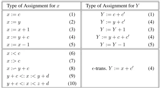
simple assignments given by table 2, page 1030. We denote by A(X) the set of clock assignments.

As defined in subsection 2.2.3, for a clock valuationv and an assignment a, we denote a(v) the clock

assignmenta(v)(x) = a(x)(v). For t ∈ R≥0the clock valuationv+t is defined by ∀x ∈ X, (v+t)(x) =

v(x) + t.

The set of clock constraintsB(X) over a set X of clocks is defined inductively by:

g := x v r| x − y v r |g ∧ g |g ∨ g (1)

withx, y ∈ X, v∈ {<, <, >, ≥, =}, r ∈ Q. Also we denote by BC(X) the subset of B(X) that defines

convex clock constraints. A clock constraint g is a particular formula and evaluates either to tt or ff : JgK ⊆ RX

≥0andg(ν) = tt ⇐⇒ ν ∈ JgK.

Timed Transition Systems and Timed Automata. A timed transition system [23] (TTS) is a tuple

(Q, E, Q0, →), where Q is set of locations, E is the set of actions, Q0 is the set of initial states,→⊆

Q × (E ∪ R≥0) × Q. A timed automaton [17] is a tuple (L, L0, E, X, I, T ) such that L is a (finite) set

of locations,X is a finite set of clocks, L0 is s.t.JL0K ⊆ L × RX≥0 is a predicate that defines the set of

initial states,E is a finite set of actions, T ⊆ L × (B(X) × E × A(X)) × L is the transition relation, I : L → BC(X) is the invariant constraint.

The semantics of a timed automaton (L, L0, E, X, I, T ) is given by a TTS (L × RX≥0, E, Q0, →)

whereQ0 = JL0K and ∀(l, v) ∈ L × RX≥0the transition relation→ is defined by: i) discrete steps of the

form(l, v) −→ (le 0_{, v}0_{) if ∃(l, g, e, a, l}0_{) ∈ T, such that g(v) = tt, v}0 _{= a(v), v}0 _{∈ JI(l}0_{)K, ii) continuous}

A very useful result about timed automata (actually updatable timed automata [24]) is that reachab-ility is decidable [17, 24] for this class of timed systems. Hence automatic verification tools have been

designed to analyse timed automata, and among themUPPAAL[5],KRONOS[7] andCMC[6]. We

will give in the last section a translation from aTimed AltaRicaspecification into a timed automaton.

This will allow us to useUPPAAL[5] orKRONOS[7] orCMC[6] to check timed properties on the

designed systems.

In the sequel, we define Timed Interfaced Transition Systems (TITS) that are extended TTS. The

timed extension ofAltaRicacomponents are timed components that are the counter parts of timed

auto-mata: the semantics of timed components is given by TITS.

3.2. Timed Interfaced Transition Systems

Timed Interfaced Transition Systems are an extension of ITS with real-valued variables and flows. Definition 3.1. (Timed Interfaced Transition System)

A timed interfaced transition system (in the sequel TITS) of continuous dimension (n, m) and time

domain4_{T is a tupleA = hE}

t, Ft, St, π, T i with:

1. Et= E+∪ {ε} ∪ T where E+is a finite set of events such thatε 6∈ E+∪ T and E+∩ T = ∅;

2. Ft⊆ F × Rmis the set of flow values, whereF is the set of discrete flow values and Rmis the set

of continuous flow values;

3. St⊆ S × Rnis the set of states whereS is the set of discrete states and Rnis the set of continuous

states;

4. π : St → 2Ft associates to each state q ∈ St all the admissible flow values in q. We assume

∀q ∈ St, π(q) 6= ∅.

5. T ⊆ St× Ft× Et× St× Ftis the transition relation and satisfies:

(a) (q, g, e, q0, g0) ∈ T ⇒ g ∈ π(q) ∧ g0 ∈ π(q0)

(b) ∀q ∈ St, ∀g, g0 ∈ π(q) we have (q, g, ε, q, g0) ∈ T

(c) ∀q ∈ St, ∀g ∈ π(q) we have (q, g, 0, q, g) ∈ T

A configuration of a TITS is a pair((s, ν), (f, µ)) ∈ St× Ftsuch that(f, µ) ∈ π(s, ν).

Remark 3.1. Compared to item 5 of Def. 2.1, we need to be more precise when defining the set of transitions of a TITS. Indeed we want to enforce discrete variables to remain unchanged when time

elapses. Assume we define the transition relation T in the same way as it was in defined item 5 of

Def. 2.1: T ⊆ St× Ft× Et× St. Then we will not be able to leave discrete flow values unchanged

during a delay transition when we define the semantics ofAltaRicatimed components (Def. 3.7): in the

target configuration, we can only constrain the state variables inStand not the flow variables inFt. Thus

we prefer to defineT over St× Ft× Et× St× Ftwhich enables us to refer to the source and target flow

values of a transition as in item 5.(c) of Def. 3.1.

4

Also note the following properties: if n = 0 and m = 0 and T = {0} we obtain the definition of

ITS. Indeed as pointed out in remark 2.1, we can give the definition of the transition relation of an ITS

in terms of transitions between configurations. Ifm = 0 and we add an initial state to the TITS then

we obtain the definition of TTS:F is to be interpreted as the set of atomic properties. It is possible to

consider an integer time domain, T= N. Notice that in this case even if we allow only integer time steps

in the TITS, the values of the clocks can be in R≥0. For a dense time domain T = Q≥0 is suitable. For

a continuous time domain one can take T= R≥0. In the following we assume the time domain is R≥0

when we deal withTimed AltaRicanodes.

3.3. Timed Bisimulations

In the sequel we will use the notion of timed bisimulations between timed systems. We define it for TITS extending the definition of interfaced bisimulation of [10]:

Definition 3.2. (Timed Interfaced Bisimulation)

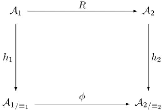
LetA1 = hEt, Ft, S1t, π1, T1i and A2 = hEt, Ft, S2t, π2, T2i be two TITS. A timed interfaced

bisimu-lation rebisimu-lation forA1andA2is a relationR ⊆ S1t × S2t that satisfies4 conditions:

1. ∀q1 ∈ S1t, ∃q2 ∈ S2t s.t.(q1, q2) ∈ R and ∀q2 ∈ S2t, ∃q1 ∈ S1t s.t.(q1, q2) ∈ R,

2. ∀(q1, q2) ∈ R, π1(q1) = π2(q2),

3. ∀(q1, g, e, q01, g10) ∈ T1, ∀q2 ∈ S2t such that (q1, q2) ∈ R then ∃(q2, g, e, q

0

2, g20) ∈ T2 s.t.

(q0₁, q₂0) ∈ R,

4. ∀(q2, g, e, q02, g20) ∈ T2, ∀q1 ∈ S1t such that (q1, q2) ∈ R then ∃(q1, g, e, q01, g10) ∈ T1 s.t.

(q0₁, q₂0) ∈ R.

Two TITS are timed bisimilar iff there exists a timed interfaced bisimulation relation on their set of states. In the sequel we use the term timed bisimulation instead of timed interfaced bisimulation. Like in the untimed case, an interfaced bisimulation can be expressed as an homomorphism between two TITS. Definition 3.3. (Timed Interfaced Bisimulation Homomorphism)

LetA1 = hEt, Ft, S1t, π1, T1i and A2 = hEt, Ft, S2t, π2, T2i be two TITS. A timed interfaced

bisimu-lation homomorphismh : A1 → A2is a mappingh : S1t → S2t such that:

1. h is surjective, 2. ∀q1 ∈ S1t, π1(q1) = π2(h(q1)), 3. ∀(q1, g, e, q01, g10) ∈ T1, ∃g20 such that(h(q1), g, e, h(q10), g02) ∈ T2, 4. ∀q1 ∈ S1t, ∀q 0 2 ∈ S2t s.t. (h(q1), g, e, q 0

2, g20) ∈ T2 then ∃q01 ∈ S1t such that h(q

0

1) = q20 and

∃g0

1∈ π1(q10) such that (q1, g, e, q10, g10) ∈ T1.

We use the term timed bisimulation homomorphism as a shorthand for timed interfaced bisimulation homomorphism.

Theorem 3.1. Two TITS A1 andA2 are timed bisimilar if and only if there exists a TITSB and two

timed interfaced bisimulation homomorphismsh1 : A1 → B and h2 : A2 → B.

The proof is given in Appendix A.1.

3.4. Timed Priorities

In the untimed version ofAltaRica, priorities among events play an important role [10]: they allow the

easy modeling of priorities among concurrently enabled transitions. It is natural in a timed setting to try and introduce timed priorities i.e. priorities among transitions involving some timing information. Again

we want to extend the existingAltaRicaspecification language and add timed priorities.

Timed priorities in timed systems have been introduced for timed automata [26] and a comprehensive study of timed priorities can be found in [27, 28, 29]. The most common timed priority is urgency [30]: basically, it says that if a transition is enabled in a timed automaton, time can not elapse and this transition

must be fired immediately. Without loss of expressiveness we define urgent events: if an event in aTimed

AltaRicaspecification is urgent then all the transitions labelled by this event are urgent. We then extend Def. 2.2 to allow priority between time labels (in T) and discrete events:

Definition 3.4. (Simple Timed Priority Relation)

A simple timed priority relation< over E is a strict partial order over E ∪ {time} such that < is a priority

relation overE and a strict partial order over Etime

+ withE+time= E+∪ {time} and ∀v ∈ E+, v 6< time.

Then a > time means5 _{that event a is urgent and has to be fired immediately when enabled (a}

semantic definition of priorities will appear later in this section in Def. 3.6). Also note that ifa > time

andb > a then b > time: the urgency of event a entails urgency of greater events.

This allows us to model what is called eagerness in [30]: an eager transition is one that forbids time elapsing if it is enabled. In the papers [27, 28] other notions of priorities are defined: (i) a delayable transition is one that can be fired when its guard is true and before a certain deadline; (ii) a lazy transition

is one that has no deadline (it may or may not be fired). We will add in Def. 3.7 (time) guards intoTimed

AltaRicacomponents which will enable us to define lazy transitions. It is proved in [28] that a delayable transition can be encoded using lazy an eager transitions. As we already know (Def. 3.4) how to define eager transitions, we are able to express the three types of priorities proposed in [30].

More elaborate ways of prioritising transitions are given in [27]. The aim is to express priority between events when several are enabled by using timing information. It is an extension of the priority

relation notion: we want to express thate < e0only ife0will not be enabled in some future. Intuitively,

we will writee <5 e0 for: the transition labellede0, if enabled within5 time units, has priority over e.

We now extend the notion of simple timed priority relation: Definition 3.5. (Timed Priority Relation)

A timed priority relation < over E is a 3-ary relation in Etime

+ × (N ∪ {∞}) × E+time satisfying the

following conditions (we denotea1<ka2for(a1, k, a2) ∈<):

• the binary relation <0is a simple timed priority relation,

5

We rule out time > a as the purpose of a priority relation is to add a sort of liveness in the system by forcing some discrete actions to be taken.

• a <kb ∧ a = time =⇒ k = 0,

• ∀k ∈ N, <kis a strict partial order,

• a1<ka2=⇒¡∀k0 < k, a1 <k0 a₂¢.

Remark 3.2. Notice that in [27], another condition can be imposed on< (a transitivity condition). This

condition is related to the building of live timed systems and is not relevant in our setting. It is aimed at preserving liveness in the systems and can then add new behaviors. We do not want to build live timed systems but only to provide a restriction operator (by giving priorities) that restricts the set of behaviors of the system. Note also we restrict the bounds to N which in theory is enough for specifying timed systems.

The static priority ofAltaRicacoincides with the particular timed priority where all the delays are equal

to zero, i.e.k = 0.

As in section 2.2.2, we define the timed priority restriction operator. Definition 3.6. (Timed Priority Restriction Operator)

LetA = hEt, Ft, St, π, T i be a TITS of continuous dimension (m, n), time domain T and < a timed

priority relation overE. We define the timed priority restriction operator ¹ for the transition relation

T ⊆ St× Ft× Et× St× Ftand the timed priority relation< by:

(q, g, e, q0, g0) ∈ T ¹<⇔ (q, g, e, q0, g0) ∈ T ∧                ife = t ∈ T, ∀t0∈ T, t0 < t, if (q, g, t0, q00, g00) ∈ T then∀e0 ∈ E+, (q00, g00, e0, q000, g000) ∈ T =⇒ time 6<0e0. otherwise if(q, g, t, q00, g00) ∈ T, t ∈ T, t ≤ k, then∀e0_{, (q}00_{, g}00_{, e}0_{, q}000_{, g}000_{) ∈ T =⇒ e 6<} ke0. We denoteA ¹< = hEt, Ft, St, π, T ¹<i.

Remark 3.3. Again, if T= {0}, we obtain the definition of the priority relation restriction (Def. 2.3).

We can lift the following theorem for ITS stated in [10] to TITS: Theorem 3.2. (Priority and Timed Bisimulation)

Let A1 = hEt, Ft, S1t, π1, T1i and A2 = hEt, Ft, S2t, π2, T2i be two TITS and < a timed priority

relation overE. If h : A1 −→ A2is a timed bisimulation homomorphism thenh : A1¹< −→ A2¹< is

also a timed bisimulation homomorphism. The proof is given in appendix A.2.

3.5. Timed Components

Timed AltaRica components are the timed extensions of AltaRica components (see Def. 2.4). Our

extension consists in adding clocks to AltaRica components. Hence our model is closely related to

the timed automaton model. Adding real-valued variables instead of clocks is quite straightforward: the resulting model is then close to the hybrid automaton model. In this paper we focus on the timed

extension and the addition of clocks. We consider the formulas F, expressions E and set of valuesD

settled in section 2.2.3.

Definition 3.7. (Timed Component)

A timed component is a tupleT = hVS∪ CS, VF ∪ CF, E, A, M, <i with:

1. VS, VF are finite sets for respectively state variables, flow variables with the property of being

disjoint. We denoteVT = VS∪ VF;CS, CF are finite sets for respectively clock variables, real

flow variables with the property of being disjoint. We denoteCT = CS∪ CF; also we assume

VT ∩ CT = ∅;

2. E = E+∪ {ε} where E+is a finite set of events and as usualε is the empty action;

3. A = AVT ∩ ACT ∈ F is an assertion such that free(A) ⊆ VT ∪ CT;AVT ∈ F, free(AVT) ⊆ VT.

ACT =

V

k∈KPk =⇒ Ik whereK is a finite set of indices, Pk ∈ F, free(Pk) ⊆ VT, Ik ∈ F,

free(Ik) ⊆ CT andIkdefines a convex region of Rpif|CT| = p;

4. M ⊆ (F × B(CT)) × E × (E(VT)VS × A(CT)) is a macro-transition relation such that every

((g, γ), e, (a, R)) ∈ M satisfies:

(a) (g, γ) is a guard such that g ∈ F and free(g) ⊆ VT;γ ∈ B(CT);

(b) e ∈ E is the event of the transition;

(c) a : VS → E(VT) is an assignment for the variables in VS. R ∈ A(CT) is the clock

assign-ment of the transition;

5. < is a timed priority relation.

Remark 3.4. Item 3 of Def. 3.7 allows us to specify constraints C between clock variables and

real-valued flow variables (e.g. Y = x where Y is a flow variable and x is clock variable): it suffices to use

tt =⇒ C where C ∈ F(CT) (e.g. tt =⇒ Y = x).

Notice that the semantics ofA is a subset of (DVS_{× R}n_{) × (D}VF _{× R}m_{) as well as the semantics of a}

guard(g, γ).

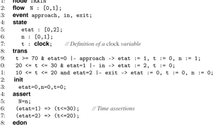
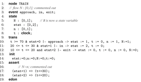
Example 3.1. (The Train)

In Fig. 4 the time features of component TRAIN appear on line 7 where a clock (state) variable t is

declared; it is used to constrain the guards of the transitions (see lines 9 to 11) and on some of themt

is reset; also the assertion (lines 16–17) implies that when in state etat= 1 (resp. 2) time cannot elapse

aftert has reached30 (resp. 20).

Definition 3.8. (Semantics of Timed Components)

LetT = hVS∪ CS, VF ∪ CF, E, A, M, <i be a timed component. Let |CS| = n and |CF| = m. The

semantics ofT over the time domain T is the timed interfaced transition system JT K = hEt, Ft, St, π, T i

of dimension(n, m) constructed in the following way:

1. Et= E ∪ T,

1: node TRAIN 2: flow N : [0,1];

3: event approach, in, exit; 4: state

5: etat : [0,2]; 6: n : [0,1];

7: t : clock; // Definition of a clock variable

8: trans

9: t >= 70 & etat=0 |- approach -> etat := 1, t := 0, n := 1; 10: 20 <= t <= 30 & etat=1 |- in -> etat := 2, t := 0;

11: 10 <= t <= 20 and etat=2 |- exit -> etat := 0, t := 0, n := 0; 12: init

13: etat=0,n=0,t=0; 14: assert

15: N=n;

16: (etat=1) => (t<=30); // Time assertions

17: (etat=2) => (t<=20); 18: edon

Figure 4. Specification of a Train as a Timed Component

3. St= {(s, ν) ∈ DVS× Rn≥0|∃(f, µ) ∈ DVF × Rm| ((s, ν), (f, µ)) ∈ JAK},

4. π : St→ 2Ftsuch thatπ(q) = {(f, µ)| (q, (f, µ)) ∈ JAK},

5. T ⊆ St× Ft× Et× St× FtandT = JM K ¹< with:

(a) lett = ((g, γ), e, (a, R)), define JtK by:

((s, ν), (f, µ), e, (s0, ν0), (f0, µ0)) ∈ JtK if            ((s, ν), (f, µ)) ∈ JA ∧ g ∧ γK ∧s0 _{= a(s, f )} ∧ ν0= R(ν, µ) ∧ (f0, µ0) ∈ π(s0, ν0)

withR(ν, µ) the new clock assignment after resetting the variables in R.

(b) letδ ∈ T, define JδK by:

((s, ν), (f, µ), δ, (s, ν0), (f, µ0)) ∈ JδK if      ((s, ν), (f, µ)) ∈ JAK ∧ν0 _{= ν + δ ∧ ((s, ν}0_{), (f, µ}0_{)) ∈ JAK} ∧∀δ0 ≤ δ, ∃µδ0| (ν + δ0, µδ0) ∈ JI(s, f )K withI(s, f ) =V_{k∈K|(s,f )∈P} kIk. (c) JM K = ∪t∈MJtKS∪δ∈TJδK.

Remark 3.5. Note thatJI(s, f )K is a convex set as it is a conjunction of convex sets. We have not used

this property ofI(s, f ) in the semantics of components as it is not required in this definition. Anyway in

the sequel we will need this assumption and this is why we have put it in Def. 3.7 of timed components. The delay transitions in the semantics of a timed components leave the “continuous” flows free

encountered along a delay transition could even be non continuous. For instance a constraint on a flow likex ≤ Y ≤ x+2 where x is a clock and Y a continuous flow would allow Y to take any value between x and x + 2 at each time point. If we define flow to be clock we constrain the set of equations we can

write in the assertion. Indeed equations likeY = 2x could not be defined with a “clock” Y . So far we

stick to this permissive definition and we will tackle later which kind of flows can be “implemented” (see section 4.4).

Finally in the caseCF = ∅ we obtain the definition of timed automata (again if we add an initial

state); the semantics of such a timed component is then a TTS (again VF is to be interpreted as some

properties or observations on each state.)

As for the untimed case we have the following lemma:

Lemma 3.1. LetT = hVS∪ CS, VF∪ CF, E, A, M, <i be a timed component and < is a timed priority

priority relation. ThenJhVS∪ CS, VF ∪ CF, E, A, M, <iK = JhVS∪ CS, VF ∪ CF, E, A, M, ∅iK ¹<.

The proof is straightforward from Def. 3.6 and Def. 3.8.

3.6. Timed Nodes

Timed nodes are straightforward extensions of nodes. Indeed, if we assume as stated in Def. 2.6 of a node, that the synchronization constraint is expanded, the new constraint added by the time transitions is

trivial: the synchronized time transitions forn nodes are of the form (δ, δ, · · · , δ), δ ∈ T where T is the

time domain and they do not need to be specified. Definition 3.9. (Timed Node)

A timed node is a tupleN = hVF, CF, E, <, N0, · · · , Nn, ( eV , <Ve)i with:

1. VF is a set of flow variables,

2. CF is the set of real flow variables,

3. E = E+∪ {ε} is a finite set of events,

4. < is a timed priority relation over E,

5. for alli ∈ [1, n], Niis a timed component or a timed node; the interface of the node is composed

of (i)VFi∪ CFi, the set of discrete flows and real flows ofNi and (ii)Ei the set of events ofNi.

We assume∀i 6= j ∈ [1, n], VFi∩ VFj = CFi∩ CFj = ∅,

6. N0 is a special timed component called the control component. The set of events of this node is

E0 = E and the priority relation of N0 is the empty relation. The set of (discrete) flow variables

ofN0 isVF0 = VF ∪ VF1 ∪ VF2 ∪ · · · ∪ VFn, and the set of real flow variables isCF0 = CF ∪

CF1 ∪ CF2∪ · · · ∪ CFn,

7. eV ⊆ E0× E1× · · · × Enis an expanded synchronization set together with a priority relation<Ve.

Remark 3.6. Notice that <_Ve is a priority relation and not a timed priority relation. This is because

( eV , <_Ve) expresses the discrete synchronization constraint.

Example 3.2. (Hierarchical Specification of the Train-Gate-Controller)

A timed version of the train-gate-controller is given in Fig. 5. Notice that the gate is a component, the

train is the component given by Fig. 1, but the nodeMAIN embeds the CONTROLLER node and plays the

role ofN0.

node GATE

event Go_down, Go_up, down, up;

state etat : [0,3]; y : clock;

trans

etat=0 |- Go_up -> ;

etat=0 |- Go_down -> etat:=1, y:=0; etat=1 |- Go_down -> ;

etat=1 & y <= 10 |- down -> etat:=2; etat=1 |- Go_up -> etat:=3, y:=0; etat=2 |- Go_down -> ;

etat=2 |- Go_up -> etat:=3, y:=0; etat=3 |- Go_up -> ;

etat=3 |- Go_down -> etat:=1, y:=0; etat=3 & y <= 10 |- up -> etat:=0;

init etat:=0, y:=0; assert (etat =1) => (y <= 10); (etat =3) => (y <= 10); edon

(a) The Timed Gate

node MAIN

flow N : [0,p];

event approach, exit, Go_up, Go_down;

priorities Go_up (<,k) approach;

state etat : [0,2]; z : clock;

trans

etat=0 |- approach -> etat:= 1, z:=0; etat=0 & N>1 |- exit -> ;

etat=0 & N=1 |- exit -> etat:= 2, z:=0; etat = 1 |- approach -> ;

etat = 1 |- exit -> ;

etat=1 & z<=10 |- Go_down -> etat:=0; etat=2 & z <= 10 |- Go_up -> etat:=0; etat=2 |- approach -> etat:= 1, z:=0;

sub t1, t2 : TRAIN, g : GATE;

sync <t1.approach,t2.approach,approach>; <t1.approach,approach>; <t2.approach,approach>; <Go_down,g.Go_down>; <t1.exit,t2.exit,exit>; <t1.exit,exit>; <t2.exit,exit>; <Go_up,g.Go_up>; init etat := 0, z := 0; assert N=t1.N+t2.N; (etat =1) => (z <10); (etat =2) => (z <= 10); edon

(b) The Timed Controller

Figure 5. Timed AltaRicaSpecifications for the Controller and the Gate

Syntactically there is not much changes between timed and untimed nodes. The differences appear in the semantics where the timed transitions are synchronized:

Definition 3.10. (Semantics of Timed Nodes)

Let N = hVF, CF, E, <, N0, · · · , Nn, ( eV , <Ve)i be a timed node and JNiK = hEit, Fit, Sit, πi, Tii

of dimension (ni, mi) for i ∈ [0, n]. The semantics of N is the timed interfaced transition system

1. Et= E ∪ T,

2. Ft= DVF × Rm, withm = |CF|,

3. forqi∈ Sit, letq = (q0, q1, · · · , qn), then

π(q) = {(f, µ) ∈ DVF _{× R}m_{| ∀i ∈ [1, n], ∃η}

i ∈ πi(qi) | ((f, µ), η1, η2, · · · , ηn) ∈ π0(q0)}

4. St= {q ∈ S0t× S1t× · · · × Snt| π(q) 6= ∅};

5. T ⊆ St× Ft× Et× St× Ftis defined by:

(a) let<0 be the timed priority relation defined by:

(e0, e1, · · · , en) <0(e00, e01, · · · , e0n) ⇐⇒ e0 < e00 (b) lete = (e0, e1, · · · , en) ∈ E0× · · · × En∪ {(δ, · · · , δ)}, s = (s0, s1, · · · , sn) and s0 = (s0₀, s0₁, · · · , s0_n). Define TN by: hs, f, e, s0, f0i ∈ TN ⇐⇒      ∃f0= (f, f1, · · · , fn) ∈ π0(s0) ∃f0 0= (f0, f10, · · · , fn0) ∈ π0(s00) ∀i ∈ [0, n], (si, fi, ei, s0i, fi0) ∈ Ti (c) thenT =¡TN¹<_V˜ ¢ ¹<0.

We have the node version of lemma 3.1:

Lemma 3.2. LetN = hVF, CF, E, <, N0, · · · , Nn, ( eV , <Ve)i be a timed node and JN K its semantics.

ThenJN K = JhVF, CF, E, ∅, N0, · · · , Nn, ( eV , <Ve)iK ¹<.

The proof is straightforward from Def. 3.9 and Def. 3.10.

The semantics of nodes is compositional with respect to timed bisimulation:

Theorem 3.3. LetN = hVF, CF, E, <, N0, · · · , Nn, ( eV , <Ve)i and N0 = hVF, CF, E, <, N00, · · · , Nn0,

( eV , <_Ve)i be two timed nodes such that ∀i ∈ [0..n] there is a timed homomorphism hifromJNiK to JNi0K.

Then there exists a timed homomorphismh from JN K to JN0K.

The proof is given in appendix A.3.

Timed AltaRicais a hierarchical modeling language so that each timed node can be expressed by a timed component. The timed priorities and the synchronization are directly encoded into the resulting timed

component. LetN = hVF∪ CF, E, <, N0, · · · , Nn, ( ˜V , <_V˜)i be a timed node, we present the

construc-tion (extending the one given in [10]) of a timed componentCN = hVS ∪ CS, VF ∪ CF, E, A, M, <i

which has the same semantics.

Definition 3.11. (Symbolic Semantics)

If N = hVF ∪ CF, E, <, N0, · · · , Nn, ( ˜V , <_V˜)i is a timed node, with Ni = hVFi ∪ CFi, Ei, <i

, Ni0, · · · , Nin, ( ˜Vi, <_V˜_i)i for 0 ≤ i ≤ n, we denote by CN = hVS ∪ CS, VF ∪ CF, E, A, M, ∅i the

timed component constructed as follows: 1. ∀0 ≤ i ≤ n

(a) ifNiis a timed component, then we defineN_i0 = Ni¹<iand the timed priority is syntactically

encoded inN_i0as defined later in section 3.7.2;

(b) ifNiis a timed node, then we defineNi0 = CNi the rewriting ofNiinto a timed component

and encode timed priority syntactically as defined in section 3.7.2;

(c) we denoteN_i0= hV_S0 i∪ C 0 Si, V 0 Fi∪ C 0 Fi, E 0 i, A0i, Mi0, ∅i; 2. VS = VS00∪ · · · ∪ V 0 Sn andCS = C 0 S0∪ · · · ∪ C 0 Sn; 3. A = (∃i=1..n(VF0i ∪ C 0 Fi)). V i=0..nA0i;

where the notation∃i=1..n(Wi).φ stands for: ∀i, ∃ηi ∈ Wi such thatφ(ηi). For ((s, ν), (f, µ)) ∈

DVS × RCS× DVF × RCF _{we define:} • ((s, ν), (f, µ)) ∈ JAK ⇐⇒ ∀i ∈ [1..n], ∃ηi ∈ DV 0 Fi _{× R}CFi0 _{s.t.((s, ν), (f, µ), η1, · · · , ηn))} ∈ JV_i=0..nA0_iK, • ∀i ∈ [1..n], ((s, ν), (f, µ), η1, · · · , ηn)) ∈ JA0iK ⇐⇒ ((si, νi), ηi) ∈ JA0iK.

4. the set of macro-transitionsM ⊆ (F×B(CT))×E ×(E(VT)VS×A(CT)) is defined by M = (M0¹

<_Ve)¹<0, where<0is the timed priority relation specified in Def. 3.10, and((g, γ), e, (a, R)) ∈ M0

if and only if:

• ∀0 ≤ i ≤ n, there is a transition ((gi, γi), ei, (ai, Ri)) ∈ Mi0such that:

– g = (∃i=1..nVFi).g0∧ · · · ∧ gn,

– γ = (∃i=1..nCFi) .γ0∧ · · · ∧ γn,

• ∀x ∈ VS∩ V_S0_i we havea(x) = ai(x) and ∀c ∈ CS∩ C_S0_i we haveR(c) = Ri(c),

• e = (e0, e1, · · · , en) ∈ eV .

Theorem 2.1 (see page 1009) for untimed nodes carries over to timed nodes:

Theorem 3.4. LetN be a timed node. Then N can be rewritten into a timed component CN such that

JN K and JCNK are timed bisimilar.

3.7. Syntactical Timed Priority

In [27] the authors show that it is possible to encode a priority relation by strengthening the guards of a component: this way one can syntactically encode the priority relation.

We tackle this problem in the timed case. LetT = hVS ∪ CS, VF ∪ CF, E, A, M, ∅i be a timed

component and< be a timed priority relation. We first assume6 _{that< contains no urgent events i.e.}

∀e ∈ E, time 6< e. Our aim is to compute the transition relation M ¹< syntactically i.e. by finding new

guards that defineM ¹<. We first rewrite our timed component so that we are sure that when a guard

evaluates to true, the corresponding transition can indeed be fired, i.e. the resulting new state satisfies

assertionA. This is done by adding weakest precondition (section 3.7.1) into the existing guards. Then

we show how to encode timed priority (section 3.7.2) again by strengthening the guards. Finally we detail how urgency is handled in section 3.7.3.

3.7.1. Weakest Precondition

The key point is to know if a transition((g, γ), e, (a, R)) can really be fired, and the fact that the guard

evaluates to true is not sufficient: a new state can be reached from((s, ν), (f, µ)), only if after the

assign-ments given by(a, R) π(a(s, f ), R(ν, µ)) 6= ∅, i.e. there are some admissible flow values. This latter

condition depends on assertionA of the timed component and can be seen as a weakest precondition.

First assume we have an untimed component (Def. 2.4). Let t = (g, e, a) be a transition of this

component, andA the assertion. For Q ⊆ S × F , we define Pret(Q) = {(s, f ) | ∃f0| (a(s, f ), f0) ∈

Q}. Assume Pret(JAK) can be defined by a formula φt ∈ F, and free(φt) ⊆ VT. Now if we take

t0 = (g ∧ φt, e, a), we are sure that when g ∧ φtevaluates to true the transitiont can be fired as (s, f ) ∈

Jg ∧ φtK =⇒ π(a(s, f )) 6= ∅.

We can extend this to the timed component. For t = ((g, γ), e, (a, R)) we define Pret(Q) =

{((s0_{, ν}0_{), (f}0_{, µ}0_{)) | ∃f}00_{, µ}00_{| ((a(s}0_{, f}0_{), R(ν}0_{, µ}0_{)), (f}00_{, µ}00_{)) ∈ Q}. Assume Pre}

t(JAK) can be

writ-ten asφt∧ θtwith free(φt) ⊆ VT and free(θt) ⊆ CT.

Then if we definet0 = ((g ∧ φt, γ ∧ θt), e, (a, R)), we can ensure that if the guard of t0 evaluates to

true,t can be fired.

Now we show how to encode Pret(JAK) into guards of the form (g, γ) with g ∈ F, free(g) ⊆ VT

andγ ∈ B(CT). Assume A = p1 ∧ p2 ∧ · · · ∧ pn∧ (q1 =⇒ i1) ∧ · · · ∧ (ql =⇒ il). Assume

Pret(JAK) is a conjunction of the form7p01∧ p02∧ · · · ∧ p0k∧ (q01 =⇒ i01) ∧ · · · ∧ (q0m =⇒ i0m). Let

P0 = p0₁∧ p0

2∧ · · · ∧ p0k. We can rewrite Pret(JAK) as8:

_ J ∪I=[1..m] I∩J=∅ P0^∧j∈J¬q0j ^ ∧r∈Iq0r | {z } GI,J ^ ∧r∈Ii0r | {z } ΓI,J

This is a formula of the formW_p=1..sGp∧ ΓpwithGp ∈ F, free(Gp) ⊆ VT andΓp ∈ B(CT). Now we

creates transitions from t = ((g, γ), e, (a, R)) defined by:

∀p ∈ [1..s], tp = ((g ∧ Gp, γ ∧ Γp), e, (a, R))

6

Urgency is dealt with in section. 3.7.3 and requires additional assumptions and definitions.

7_{Quantifier elimination in Pre}

t(JAK) can only be done under some conditions (e.g. the discrete domain is finite). We do not

discuss this in this paper and assume we can actually find a quantifier-free expression for Pret(JAK).

8

It remains to replacet by the tp, p ∈ [1..s] to build a new timed component and t can be fired in the

original component if and only if one of thetp can be fired in the new component (leading to the same

values for the state variables.) In the sequel we assume guards have been strengthened so that if a guard evaluates to true then the transition can actually be fired.

3.7.2. Encoding Timed Priority

The Simple Case. Lett = ((g, γ), e, (a, R)) ∈ M . Assume e <k e0 and there is only one transition

t0 = ((g0, γ0), e0, (a0, R0)) ∈ M labelled with e0. Thent can be fired from a configuration q only if (g, γ)

is true inq and:

1. eitherg0is not true inq,

2. org0is true inq and γ0will not be true withink time units.

First we deal with the discrete part of the guard and split the transitiont into t1 andt2with:

• t1= ((g ∧ ¬g0, γ), e, (a, R)) which corresponds to item 1 above;

• t2= ((g ∧g0, γ), e, (a, R)) which corresponds to item 2 above although γ needs to be strengthened

to meet the requirements of item 2 above.

We now show how to strengthenγ in t2. A useful operator was introduced in [28, 29] for this purpose:

Definition 3.12. (Modal Operator [28, 29])

LetX = {x1, x2, · · · , xn}. Let ν ∈ Rnandk ∈ N. Let φ ∈ B(X) and T be the time domain. We define

the (state) predicate 3kφ by:

(3kφ)(ν) ⇐⇒ ∃t ∈ T, t ≤ k, φ(ν + t)

Now we strengthen the guardγ in t2 and define t02 = ((g ∧ g0, γ ∧ (¬3kγ0)), e, (a, R)). According

to [28, 29], it is possible to eliminate the existential quantifier in 3kγ0 and to obtain a quantifier-free

formula (we will not get into the details and refer the reader to [28, 29]).

General Case. In the general case there could bep transitions t0_i = ((g_i0, γ_i0), ei, (a0i, R0i)) s.t. e <k1

e1, · · · , e <kp ep. Then we splitt into 2ptransitionstF = ((gF, γF), e, (a, R)) with F ⊆ [1..p]:

gF = g ∧ ^ i∈[1..p]\F ¬g_i0∧ ^ i∈F g0_i (2) γF = γ ∧ ^ i∈F ¬3kiγ 0 i (3)

Remark 3.7. As stated in remark 3.2, page 1014, we do not modify the invariants of the system.

According to [27], the formula 3kγ can be written as simple formula in B(CT). If we denote by M ¹<

the transition relation obtained by:

2. strengthening the guards to encode the timed priority relation as defined above in this subsection,

we obtain a new timed componentT ¹<= hVS∪ CS, VF ∪ CF, E, A, M¹<, ∅i such that:

Lemma 3.3. (Syntactical Priority)

JT ¹<K = JT K¹<.

Lemma 3.3 follows from Def. 3.10 and Def. 3.12. From lemma 3.1, we obtain the following corollary:

Corollary 3.1. JhVS∪ CS, VF ∪ CF, E, A, M, <iK = JhVS∪ CS, VF ∪ CF, E, A, M, ∅i¹<K

This completes the syntactical encoding of timed priority without urgency for timed components.

3.7.3. Encoding Urgency

Urgency consists in preventing time elapsing when a discrete transition is enabled. In this section we

assume the time domain is R≥0. Also we assume time determinism and denoteν −t the valuation defined

by(ν −t)(x) = ν(x)−t (time non determinism is more technically involved but can be handled as well).

Our work is based on previous papers by S. Bornot, J. Sifakis and S. Tripakis [28, 29, 27]. The authors define the notion of rising edge of a guard that plays a central role:

Definition 3.13. (Rising Edge [27])

LetX = {x1, x2, · · · , xn}, ν ∈ Rnandγ ∈ B(X). The rising edge of γ, denoted γ↑ is the predicate

defined by:

γ↑ (v) =¡γ(v) ∧ ∃t > 0 , ∀0 < t0≤ t, ¬γ(v − t0)¢∨¡¬γ(v) ∧ ∃t > 0, ∀0 < t0 ≤ t, γ(v + t0)¢ (4)

We assume that each guard of a transition labelled by an urgent event is such that Jγ ↑K ⊆ JγK.

Indeedx > 10 is not a relevant guard for an urgent transition as there is no first instant at which the

guard becomes true: the transition becomes urgent strictly after10 which is a fuzzy instant and this is

in contradiction with urgency. Note that in this case (x > 10) ↑ ≡ (x = 10) which gives the same

rising edge as for x ≥ 10 but the latter has a first instant for which it is true. This problem is

well-known and is already discussed in [29]. Note that in this case equation (4) of Def. 3.13 simplifies in

γ ↑ (v) = ¡γ(v) ∧ ∃t > 0 , ∀0 < t0 ≤ t, ¬γ(v − t0₎¢_{. We also assume that a guard γ of an urgent}

transition is convex and this implies thatγ↑ is convex as well.

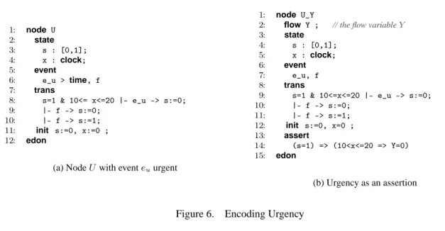
Urgency as an assertion The semantics of urgency (see Def. 3.6) implies that when a transition

be-comes urgent (i.e. its guard is true) time elapsing is forbidden and this is the semantics proposed in [29]. It does not imply that the urgent transition is fired. Also this notion is different from the notion of urgency inUPPAAL[20] which only constrains processes to synchronize on common channels (synchronized events) whenever they can.

To be more precise assume we have a component U with an urgent transition eu as defined on

Fig. 6(a).

Start in configuration(s = 0, x = 0). At some point f can occur. If it occurs before x = 10 it is

possible to let some time elapse untilx = 10 reaching (s = 1, x = 10). At this point the urgent transition

1: node U 2: state 3: s : [0,1]; 4: x : clock; 5: event 6: e_u > time, f 7: trans 8: s=1 & 10<= x<=20 |- e_u -> s:=0; 9: |- f -> s:=0; 10: |- f -> s:=1; 11: init s:=0, x:=0 ; 12: edon

(a) Node U with event euurgent

1: node U_Y

2: flow Y ; // the flow variableY

3: state 4: s : [0,1]; 5: x : clock; 6: event 7: e_u, f 8: trans 9: s=1 & 10<=x<=20 |- e_u -> s:=0; 10: |- f -> s:=0; 11: |- f -> s:=1; 12: init s:=0, x=0 ; 13: assert 14: (s=1) => (10<x<=20 => Y=0) 15: edon (b) Urgency as an assertion

Figure 6. Encoding Urgency

configuration the urgent event eu is no more enabled and time can elapse. Thus to use our notion of

urgency to force a transition to occur, one must ensure that once an urgent transition is enabled (x = 10)

no other transition can disable it (to achieve this, one could change the enabling conditionTrue of line`9

of nodeU to x<10).

To encode urgency, we use an additional real flow variable Y (see line 2 of Fig. 6(b)). This flow

variable is assumed to be reset to0 on each discrete transition and evolves at rate 1 (synchronous with

physical time) on delay transitions. How this will be achieved will be dealt with later in this section.

The syntactical encoding of urgency consists in adding a timed invariant (line 14 of nodeU_Y, Fig. 6(b))

to constrain time elapsing. Note that this assertion implies Y = 0 only when x > 10 (and not x ≥

10). Intuitively, assume we reach a configuration (s = 1, x < 10). Then time can elapse from this

configuration untilx = 10. Indeed (s = 1, x = 10) satisfies Def. 3.6 as for each strictly preceding

instant the assertion is true. From this configuration on time cannot elapse asY > 0 and the assertion

forbids it. Now if we reach(s = 1, 10 ≤ x ≤ 20) by firing a discrete transition, Y is set to 0 and time

elapsing is also forbidden. This achieves urgency (in the sense that time elapsing is prevented).

Some limitations of our encoding is that we do not know how to deal with urgent transitions with

sharp urgent guards asx = 5. This is why we require an additional assumption on guards for urgent

transitions: the (temporal) guardγumust satisfy∃² > 0 , ν ∈ Jγu↑K =⇒ ∀²0 ≤ ² ν + ²0 ∈ JγuK. We

refer to this latter property asγuis not sharp.

Correctness of the encoding LetT = (VS∪ CS, VF∪ CF, E, A, M, <) be a timed component where

< consists in one element: eu > time (eu is urgent). Assume there is one urgent transition tu =

((gu, γu), eu, (au, Ru)), γu is not sharp, and there is a flow variableY that is reset on each discrete

transition and evolving at rate1 on delay transitions.

Define the timed component Tu = (VS ∪ CS, VF ∪ CF, E, A ∧ ϕu, M, ∅) with ϕu

def

= gu =⇒

¡

(γu∧ ¬(γu↑)) =⇒ Y = 0

¢

. Note that we assumeY is an invisible variable that does not belong to

for timed interfaced transition systems that do not have the same sets of flow variables (remind that Def. 3.2 imposes the two systems to have the same interface).

Theorem 3.5. JT K and JTuK are timed bisimilar.

The proof is given in appendix A.5.

Implementation of the encoding To implement our encoding and add a fresh flow variableY , we

proceed as follows:

1. create nodeU_Y from node U, as described by Fig. 6(b),

2. build a new nodeYY (Fig. 7(a)) that manages a variableY that satisfies the assumptions we needed

before: Y is reset on each discrete transition and evolves at rate 1 on delay transitions. Each

discrete event of other components will be synchronized with eventu of YY;

3. build a parent nodeUU that synchronizes U_Y and YY; this node is given in Fig. 7(b).

node YY flow Y; event u; state y : clock; trans |- u -> y:=0 ; init y:=0; assert Y=y edon (a) Node YY node UU event e_u,f;

sub CU_Y:U_Y; C_YY:YY;

sync <f,C_YY.u,CU_Y.f>; <e_u,C_YY.u,CU_Y.e_u>; assert CU_Y.Y=C_YY.Y edon (b) Node UU

Figure 7. Hierarchical Modeling of Urgency

This scheme can be carried out for multiple urgent events. We do not detail this in this paper as it is just a technical exercise.

Now that we know how to encode timed priority syntactically and how to flatten a node into a component. We proceed with a translation of timed components into timed automata. This will enable us to check various timed properties.

4.

From Timed Nodes to Timed Automata

In this section, we present a translation ofTimed AltaRicaspecifications to timed automata [17]. This

way we can extract a timed automaton from aTimed AltaRicaspecification and carry out some

veri-fication of temporal properties using tools for analysing timed systems likeUPPAAL[5], CMC[6] or

KRONOS [31]. Notice that thanks to theorem 3.4 we only need to define the translation for timed components.