Metric and latticial medians

HAL Id: halshs-00408174

https://halshs.archives-ouvertes.fr/halshs-00408174

Submitted on 29 Jul 2009

HAL is a multi-disciplinary open access archive for the deposit and dissemination of sci-entific research documents, whether they are pub-lished or not. The documents may come from teaching and research institutions in France or abroad, or from public or private research centers.

L’archive ouverte pluridisciplinaire HAL, est destinée au dépôt et à la diffusion de documents scientifiques de niveau recherche, publiés ou non, émanant des établissements d’enseignement et de recherche français ou étrangers, des laboratoires publics ou privés.

Bernard Monjardet, Jean-Pierre Barthélemy, Olivier Hudry, Bruno Leclerc

To cite this version:

Bernard Monjardet, Jean-Pierre Barthélemy, Olivier Hudry, Bruno Leclerc. Metric and latticial me-dians. Denis Bouyssou, Didier Dubois, Marc Pirlot, Henri Prade. Decision-making Process: Concepts and Methods, Wiley, pp.811-856, 2009. �halshs-00408174�

6.1. Introduction

The previous chapter of this book dealt with some aggregation problems arising in the field of collective choice or multicriteria decision. This chapter studies a family of aggregation methods often met in literature and which may be qualified as median procedure. In this introduction, we first consider the concept of median in general, then the medians of binary relations, and last latticial medians.

6.1.1. Medians, in general

The concept of median comes first from geometry. Every one of us dealt in school with special lines in triangles. An angle bisector cuts an angle into two equal angles and comes to an end on the opposite side. An altitude is a straight line through a vertex and perpendicular to the opposite side. A median is a straight line through a vertex and the midpoint of the opposite side, which is divided into two equal parts. More generally, medians are based on equal shares. The median of a sorted statistical series divides it into two equal parts. In their famous Dictionary of statistical terms, Kendall and Buckland [KEN 57] distinguish between “median” and “median centre” by writing that, “according to the Italian tradition”, the median centre is a point such that the sum of the distances to the points of a given set is minimum. In fact, these two notions coincide, as already pointed out by Laplace [LAP 1774]. So medians relate two kinds of structures: an ordinal structure (here, a

1 _{Chapter written by Olivier HUDRY, Bruno LECLERC, Bernard MONJARDET and Jean-Pierre}

BARTHÉLEMY. Olivier Hudry would like to thank Lucile Denœud-Belgacem very much for her help in the translation of his part of this chapter.

linear order; more generally, a lattice or a semilattice) and a metric structure (we will speak about metric median in this case). It is entertaining to observe that, if the median is of metric nature, it is not of geometric nature: the intersection of the three medians of a triangle is its centre of gravity and not the (metric) median of its three vertices. Moreover, the median of aligned points depends only on the succession of these points and not on the lengths of the intervals between them.

6.1.2. Medians of binary relations

The problem of the aggregation of binary relations (here, finite complete preorders) has been formally raised by Arrow [ARR 51]. The notion of median occurred quickly in the prolongation of this work and according to the two above mentioned dimensions: ordinal and metric. With respect to the first, Guilbaud [GUI 52] dated back the Arrowian questions to the voting theories developed at the end of 18th century by Borda [BOR 1784], Condorcet [CAR 1785] and some others (see [BLA 58]). Especially, Guilbaud insisted on the fact that the majority rule is not generally applicable, and he added: “The analytic study of Condorcet’s paradox will lead us to perceive how one can build a median in various partially ordered structures”. Indeed, Condorcet (and some others after him) noticed that the usual voting procedures made possible the election of a candidate defeated by another by a majority of voters. Then, Condorcet proposed to split the vote into duels (i.e. to compare the candidates pairwise) and to consider the candidate defeating all the others by a majority as the winner. Unfortunately, Condorcet realized that this voting procedure raised a major difficulty, called Condorcet’s effect by Guilbaud (and “voting paradox” in the English literature): it can happen that each candidate is defeated majoritarily by another one (cf. an example in Section 6.2.4).

At the end of the fifties, Kemeny [KEM 59] introduced the notion of metric median of linear orders in order to palliate Arrow’s impossibility result. This notion of median is based on the symmetric difference distance, a distance given by the number of “disagreements” between two binary relations. Kemeny’s justification to use this distance was based on its axiomatic characterization. Since these pioneer works, the works on the median of binary relations have considerably increased. One will find in [BAR 81] a review of the already abundant literature devoted to this subject before the eighties

.

From an algorithmic point of view, observe finally that, except some rather obvious cases, the search of a median (in Kemeny’ sense and for various types of binary relations) leads generally to NP-hard problems (see references in [HUD 08a]).

6.1.3. Medians in lattices

As it is usual in mathematics, the understanding of a strong relation between two approaches is reached with the help of an abstract scheme in which both approaches embed. Here, the abstract model of lattices (and semilattices) will join ordinal (Guilbaud) and metric (Kemeny) approaches. In two seminal papers, Barbut ([BAR 61] and [BAR 67]) showed that Laplace’s result, on the equivalence of ordinal and metric medians (of a series of numbers), generalizes to distributive lattices. Moreover, he explicitly related these medians, on the one hand, with Condorcet’s majority rule, and, on the other hand, with ordinal statistics as developed by Kendall [KEN 38] (the celebrated Kendall coefficient τ is nothing but a normalization between –1 and +1 of the symmetric difference distance, which was later extensively considered by Kemeny). Then, Barbut’s results were systematized by Monjardet who introduced, among others, the notion of median interval [MON 80]. Significant extensions were then developed into two directions:

– to larger types of ordinal structures, especially to modular lattices (and semilattices);

– to the study of medians in trees (a topic initiated, with no doubt, by Camille Jordan [JOR 1869]).

Finally, any statement simultaneously valid in trees and in distributive lattices may be expected to remain valid in the more general abstract structure of median semilattices (previously considered by Sholander [SHO 54] and Avann [AVA 61]). For instance, Barbut’s results on distributive lattices, together with those of Zelinka [ZEL 68] and Slater [SLA 78] on trees, were extended to median semilattices by Bandelt and Barthélemy [BAN 84].

The topic considered in this chapter is very prolific. Barthélemy and Monjardet’s paper [BAR 81] written more than twenty years ago contained about 200 references. Their number has surely at least tripled (in particular cluster analysis is become a big consumer of medians). So, we have been forced to drastic choices. On the relational side, we essentially restrict the field to the cases of arbitrary binary relations, tournaments and linear orders (nevertheless other relations occur in the last section as an application of the latticial median). On the metric side, we insist on the symmetric difference distance and its extension to semilattices. We do not deal with the “geodesic” aspects (for example, in the permutohedron lattice) which refer as well to graph theory as to ordered set theory. On the latticial side, we insist on the structure where medians have a natural algebraic expression, namely the median semilattices. This is not a reason to forget that similar or more general results (in semimodular and even arbitrary semilattices) have been obtained more or less recently (see, for example, [LEC 93] and [LEC 94]).

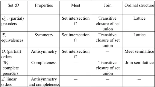
This chapter is divided into five sections, including this introduction. Section 6.2 gives the general frame, with the main definitions that will be useful later, and includes a study of the medians, in the simple cases of general binary relations and tournaments. Section 6.3 deals with median (linear) orders, and especially considers the problem of their effective computation. It includes developments about several questions relevant from a combinatorial optimization point of view. Medians in (semi)lattices are considered in Section 6.4. It is first observed that several sets of binary relations, conveniently ordered, are lattices or semilattices. Then, the attention moves from binary relations to lattices. First, the extension of the symmetric difference metric to lattices involves a definition of medians in such structures. We focus on median semilattices, previously mentioned as a privileged frame for the unification of almost all the “positive” results of the literature. This section also comes back on the uses, pointing out how the lattice approach may provide results about several types of binary relations, but also about other models of preferences (for instance, some types of choice functions). Finally, in the conclusion of the chapter, we recapitulate the different notions of medians encountered, their relationships and the situations where the median procedure turns out to be an easy method.

6.2. Median relations  6 . 2 . 1 . The model

We consider in this chapter

– a finite set V = {1, 2, …, v} of v elements henceforth called voters, but which could also be agents, criteria, etc.

– a finite set X = {x, y, z, ...} of n elements henceforth called candidates, but which could also be decisions, objects, etc.

Each voter is assumed to compare the candidates pairwise. So his preferences between the candidates are expressed by a binary relation R defined on X . One assumes that R belongs to a given set D of binary relations defined on X. So if R  =  P(X2_{) is the set of all the subsets of X}2 _{i.e., the set of all binary relations} defined on X , one has D ⊆R. When the preference relation Ri of each voter i is given, we obtain the so-called profile of the individual preferences of the voters. We denote such a profile by Π  = ( R1, R2, ...,  Rv). Thus the set of all the possible preferences profiles is Dv.

The collective preference must often belong to the same set of relations as the individual preferences i.e., it must belong to D. But we can also allow the collective relation to belong to a set M (for “models”) of relations, with generally D ⊆ M ⊆ R. Then, an aggregation procedure is a map from Dv _to M. Later on, we will need

to extend this definition by considering that the aggregation procedure can lead to several collective preference relations for the same profile of individual preferences. Then, an aggregation procedure becomes a map from Dv _{to P*(}M ), where P*(M ) denotes the set of nonempty subsets of M .

The applied aggregation procedure is required to satisfy “good properties”. For instance, if all the voters prefer a candidate to another one, this unanimous preference must be kept in the collective preference. To find “good” aggregation procedures is not an easy task. Indeed, we face strong obstacles like the “effet Condorcet” (see Section 6.3) or Arrow’s theorem [ARR 51] (see, for instance, Chapter 5 of this book and the papers in the issue 163 of Mathématiques et Sciences humaines [MSH 03]). Then we cannot be too ambitious on the qualities of the considered aggregation procedures.

The aggregation procedures that we are going to study in this chapter belong to the large class of the so-called metric aggregation procedures. They are based on a very natural idea found in various contexts, for example in data analysis. We look for the collective preference that is the “closest” –in a sense to specify– to the profile of individual preferences. In order to specify this closeness, we begin by defining a distance d on the set M of possible collective preference relations, which thus becomes a metric space (M, d). Afterwards in this metric space we define a remoteness (see [BAR 81]) between a profile of individual preferences and an arbitrary relation of M. The collective preference relations associated with this profile are the relations of M minimizing this remoteness.

6.2.2. The median procedure

Let (M, d) be the metric space where M is the set of all possible collective preference relations and d a distance on M. The median procedure is the metric aggregation procedure where the remoteness E(Π, R) between a profile Π  = ( R1, R2, ...,  Rv) of individual preferences and a relation R of M is obtained as the sum of the distances of the relations Ri of this profile to the relation R:

E(Π, R) = d(Ri, R) i=1

v

∑

.

DEFINITION 6.1.– Let Π ∈ Dv be a profile of individual preferences and M  ⊆  R. An M-median of Π is a relation of M that is a solution of the following optimization problem: minimize {E(Π, M): M ∈ M }.

As M is a finite set, there always exists at least one M-median of a profile and there can exist several M-medians. We denote by Med_M(Π) the set of M-medians of a profile Π. Obviously, the M-medians of a profile depend on the chosen distance d on M. Hereafter, we will only consider the most natural and used distance between binary relations, namely the symmetric difference distance δ. Recall the definition of this distance. Let R and R′ be two binary relations defined on a set X and RΔ ′ R be their symmetric difference. Then,

δ(R, R′ ) = RΔ ′ R = R∪R′  – R∩R′  = R \ R′  + R′ \ R, what can also be written:

δ R, ′

(

R

)

=

|

{(x, y): [(x, y) ∈ R and (x, y) ∉ ′ R )] or [(x, y) ∉ R and (x, y) ∈ ′ R )]}

|

. In other words, the symmetric difference distance between R and R ′ is the number of ordered pairs of X belonging to one of these relations and not to the other. It counts the number of disagreements between these two relations.

Then, for the chosen distance δ, the remoteness of a profile Π  = ( R1, R2, ...,  Rv) to a relation R is:

E(Π, R) = δ( Ri, R) i=1

v

∑

.

6.2.3. The R -medians of a profile of relations

We begin by considering the case where the individual preferences of the voters on the candidates can be arbitrary binary relations i.e., D = R. This case, unrealistic in a voting context, can be achieved for other aggregation contexts. Moreover the results obtained for this case remain valid for particular relations. We need to define parameters associated to a profile Π = (R1, R2, ...,  Rv). We set:

Π

V (x, y) = {i ∈ V: x Ri y}, c

V_Π(x, y) = {i ∈ V: (x, y) ∉ Ri},

Π

v (x, y) = |V_Π(x, y)| = |{i ∈ V: x Ri y}|, c

v_Π(x, y) = |V_Πc(x, y)| = |{i ∈ V: (x, y) ∉ Ri}|,

Π

w (x, y) = v_Π(x, y) – vc_Π(x, y).

So, V_Π(x, y) is the set of voters preferring candidate x to candidate y, v_Π(x, y) is the number of these voters and v_Πc (x, y) is the number of voters that do not prefer x

to y (what, generally, does not mean that they prefer y to x). One has obviously v_Π(x , y )  +  v_Πc (x, y) = v and w_Π(x, y) = 2v_Π(x, y) – v. When there is no risk of ambiguity i.e., almost always, we drop the index Π in the above notation (for example, V_Π(x,y) becomes V(x, y)).

A first result states the remoteness of a profile to an arbitrary relation R by means of the previous parameters, and the changes in this remoteness when an ordered pair is removed from or added to R.

LEMMA 6.2.– For Π = (R1,  R2,  ..., R v) ∈ Rv and R ∈ R, we have:

(a) E(Π, R) = vc_{( x, y)} ( x, y)∈R

∑

+ v( x, y) (x, y)∉R

∑

; (b) E(Π, R) = Ri i=1 v

∑

− w( x, y) ( x, y)∈R

∑

;

(c) if (x, y) ∈ R, E(Π, R \ {(x, y)}) = E(Π, R) + w(x, y); (d) if (x, y) ∉ R, E(Π, R ∪ {(x, y)}) = E(Π, R) – w(x, y). Proof

Let us first prove (a). By definition of E(Π, R), we have: E(Π, R) = δ( Ri, R) i=1 v

∑

= R_iΔR i=1 v

∑

.

Let us introduce the characteristic function δi of RiΔR defined by:

∀ x, y

(

)

∈ X2, δi(x, y) = 1 if (x, y) ∈ RiΔR and δi(x, y) = 0 otherwise. Then: E(Π, R) = δi( x, y) (x, y)∈X

∑

2 i=1 v

∑

.

By partitioning X2 _{into R and its complement X}2_{\R, we obtain:} E(Π, R) = δi(x, y) i=1 v

∑

( x, y)∈R

∑

+ δi(x, y) i=1 v

∑

( x, y)∉R

∑

= vc( x, y) ( x, y)∈R

∑

+ v( x, y) ( x, y)∉R

∑

,

what proves the first relation. Adding and subtracting v( x, y) ( x, y)∈R

∑

, we obtain (b): E(Π, R) = v( x, y) ( x, y)∈R

∑

+ v( x, y) ( x, y)∉R

∑

– v( x, y) (x, y)∈R

∑

− vc_{(x, y)} (x, y)∈R

∑

        = v( x, y) ( x, y)∈X

∑

2 – w( x, y) ( x, y)∈R

∑

= Ri i=1 v

∑

– w( x, y) ( x, y)∈R

∑

.

Formulas (c) and (d) are immediate consequences of (b). ❑

In the simple cases, the median relations of a profile are linked to the “majority” relations associated to this profile. We define now these relations after introducing some notation:

for Π ∈ Rv _{and for an integer σ, we set:}

R(Π, σ) = {(x, y) ∈ X2_{: v(x, y) ≥ σ}.}

Here we also generally denote simply this relation by R(σ). It contains all the pairwise preferences supported by at least σ voters. On the other hand, if r is a real number, the notation r  (respectively r  ) denotes the integer part by excess (respectively by defect) of r. Finally, we set α=

_

( +ν 1)/2

_

and



( +ν 1)/2



=

β (thus, if v = 2p + 1, α = β = p + 1; if v = 2p, α = p + 1 and β =  p).

DEFINITION 6.3.– For Π ∈ Rv_{, the strict majority relation associated to Π is the}

relation

R(α) = {(x, y) ∈ X2: v(x, y) ≥ α=

_

( +ν 1)/2

_

}

and the majority relation associated to Π is the relation

R(β) = {(x, y) ∈ X2_{: v(x, y) ≥ β=}

_

_{( +ν 1)/2}

_

_}.

A candidate x is thus preferred to a candidate y in the strict majority relation (respectively, in the majority relation) if the number of voters preferring x to y in profile Π is strictly greater than (respectively, greater than or equal to) half the voters. Obviously, these two relations are the same if the number of voters is odd. We have also the equalities:

R(α) = {(x, y) ∈ X2_{: v(x, y) > v}c_{(x, y)} = {(x, y) ∈ X}2_{: w(x, y) > 0}} and R(β) = {(x, y) ∈ X2_{: v(x, y) ≥ v}c_{(x, y)} = {(x, y) ∈ X}2_{: w(x, y) ≥ 0}.}

The set R(β) \ R(α) = {(x, y) ∈ X2: w(x, y) = 0} is the set of the ordered pairs (x, y) of candidates for which there are as many voters preferring x to y as voters not preferring x to y. In the case where, for all the voters, x is not preferred to y if and only if y is preferred to x, R(β) \ R(α) is the set of the ordered pairs of candidates which are ex æquo, i.e., of candidates for which the numbers of voters preferring one of the candidates to the other are equal.

After a recall of the notion of interval in a lattice (see below Section 6.4.1 for the definition of a lattice), we can state the first result on the (arbitrary) medians of a profile of (arbitrary) relations. In the Boolean lattice (R, ⊆) of all the binary relations defined on X , the interval [S, T] associated to two relations S and T satisfying S ⊆ T is the set {R ∈R: S ⊆ R ⊆ T}.

PROPOSITION 6.4.– Let Π ∈ Rv _{be a profile of binary relations on X. We have:}

Med_R(Π) = [R(α), R(β)].

The number of R-medians of Π is 2|R(β)\R(α)|. If R(β) \ R(α) = ∅ (in particular if the number of voters is odd), then Π has a unique median.

Proof.

Let R be an R-median of Π. If R(α) ⊆ R is not satisfied, there exists (x , y ) ∈   X2 _{with w(x, y) > 0 and (x, y) ∉ R. By Lemma 6.2 (d), we have:}

E(Π, R ∪ {(x, y)}) = E(Π, R) – w(x, y) < E(Π, R),

what is impossible, since R is a median of Π. Likewise, if R ⊆ R(β ) is not satisfied, there exists (x, y) ∈ X2 _{with (x, y) ∈ R and w(x, y) < 0. By Lemma 6.2} (c), we have:

E(Π, R \ {(x, y)}) = E(Π, R) + w(x, y), and still a contradiction.

So, the R-medians of Π are in the interval [R(α), R(β)] and, since all the relations R of this interval have the same remoteness to the profile (i.e., E(Π, R) =  E(Π, R(α)) = Ri

i=1 v

∑

– w( x, y)

w( x, y)> 0

∑

), this interval provides all the R-medians of Π.

And since we may add or not any element of R(β) \ R(α) to form an R-median

of Π, we immediately get the number of these R-medians. ❑

The R-medians of Π are thus all the relations between the two majority relations of Π. They form the interval [R(α), R(β)] – called the median interval – of the Boolean lattice (R , ⊆) of all the binary relations. The last section of this chapter will come back on the links between medians and lattices, but we can already observe that the majority relations are obtained by means of the operations of this lattice i.e., by means of the union and of the intersection of relations. Indeed, we have

( )

U I

α ≥ ⊆ ∈         = α W V W i W i R R and and

( )

U I

β ≥ ⊆ ∈         = β W V W i W i R R and .

6.2.4. The M -medians of a profile of relations

We now consider the case where the collective preference relations associated to a profile Π are not arbitrary relations but must belong to a given set M of binary relations i.e., must be the M-medians of Π. We can always consider the R-medians of Π i.e., the median interval [R(α), R(β)], but this interval may contain no relation belonging to M. For example, if D and M are both the set of the linear orders on three candidates x, y and z, it is easy to see that the R-medians of the profile formed by the three linear orders x > y > z, y > z > x and z > x > y is the reflexive relation R defined by xRy, yRz and zRx; this relation is not a linear order (it is a 3-cycle!). In fact we have the following, obvious but not uninteresting, result:

PROPOSITION 6.5.– Let Π ∈ Rv _and M ⊆ R. If M ∩ Med

R(Π) ≠ ∅, then Med_M(Π) = M ∩ Med_R(Π).

Proof.

Indeed, if a relation of M belongs to the median interval of a profile Π, then this relation (as well as all the other relations of M belonging to this interval) minimizes the remoteness of the profile to any relation of M, since it minimizes this

remoteness on the set of all binary relations. ❑

6.2.5. The T-medians of a profile of tournaments

We now restrict the relations modelling the individual and collective preferences of the voters by assuming that they are tournaments. A tournament T on X is a complete (i.e., xTy not satisfied implies yTx) and antisymmetric (i.e., xTy and yTx

imply x = y) relation. A tournament that is also transitive (i.e., xTy and yTz imply xTz) is a linear order (the classical – and simplest – model of transitive preference). But preference relations which are non-transitive tournaments often appear, for instance when a voter is asked what his preferred candidate is in each pair of candidates (it is the so-called paired-comparison method). We denote by T (respectively, L) the set of tournaments (respectively, linear orders) defined on X. It immediately follows from the properties of tournaments that, for a profile Π  = ( T1, T2, …, Tv) ∈ Tv (and in particular for Π ∈ Lv), we have for all x and y:

c

v_Π(x, y) = v_Π(y, x) if x ≠ y; v_Πc (x, x) = 0;

Π

w (x, y) = 2v_Π(x, y) – v; w_Π(x, x) = v;

v_Π(x, y) + v_Π(y, x) = v if x ≠ y; v_Π(x, y) + v_Π(y, x) = 2v if x = y.

As above, when there is no risk of ambiguity i.e., almost always, we omit the index Π in the notation. The remoteness of a tournament T to a profile of tournaments Π = (T1, T2, …, Tv) is then given by:

E(Π, T) = v y, x

(

)

( x, y)∈T

∑

+ v x, y

(

)

( x, y)∉T

∑

= v.n (n +1) 2 –_{( x, y)∈T}

∑

w( x, y).

With this formula and Proposition 6.5, we easily find all the median tournaments of a profile of tournaments i.e., all the tournaments T minimizing E(Π, T) in the set T of all the tournaments defined on X.

PROPOSITION 6.6.– Let Π ∈ Tv be a profile of tournaments. Then Med_T(Π) = T ∩[R(α), R(β)]. Moreover, the number of median tournaments of Π is 2|R(β) \ R(α)|/2. The remoteness of a median tournament T to the profile Π is:

E(Π, T) = v.n (n +1)

2 –_{w( x, y)> 0}

∑

w( x, y). Proof.

By Proposition 6.5, we have only to show that there always exists a tournament in the median interval [R(α), R(β)] of Π. Yet, we obtain such a tournament by adding, to the antisymmetric relation R(α), one and only one of the two ordered pairs (x, y) and (y, x) whenever x and y are ex æquo i.e., when v(x, y) = v(y, x). ❑

6.3. The median linear orders (L-medians) of a profile of linear orders

Let us consider now the case for which the voters’ preferences are linear orders. Since linear orders are particular tournaments, we can apply the previous results to find the median tournaments of a profile Π of linear orders. These are the tournaments belonging to the median interval of Π, which contains always some tournaments, according to Proposition 6.6 stated above.

Everything may change if we search now for the median linear orders of Π i.e., the linear orders L minimizing E(Π, L) among the set L of linear orders defined on X. Indeed, as shown in the example given in Section 6.2.4 (before Proposition 6.5), the median interval of a profile of linear orders may contain no linear order (in this example, the median interval is reduced to the majority relation, and this single tournament is a circuit i.e., a directed cycle). We must then distinguish between two cases. In the first case, there exists a linear order in the median interval of Π or, equivalently, the strict majority relation R(α) of Π has no circuit. In this case (according to Proposition 6.6), the median orders of Π are all the linear orders belonging to the median interval, i.e. all the linear orders that contain the relation R(α) (it is well-known that a relation is contained in a linear order if and only if the relation has no circuit). The second case is the one where the median interval of the profile contains no linear order or, equivalently, the case where the strict majority relation contains a circuit. In this case, we say that a Condorcet effect occurs2_{. The} possible existence of a Condorcet effect has the following consequence. Whereas obtaining median relations or median tournaments of a profile was easy, the problem consisting in searching for a median linear order becomes hard (actually NP-hard, see Section 6.3.4) and requires the study of the properties of such orders and the use of combinatorial optimization methods to provide exact or approximate solutions. This issue will be the subject of this section (Section 6.3); in Section 6.4, we will come back to the “easy” case, which can be dealt with in the framework of “median semilattice”.

2 _{The possible existence of circuits in the majority relation was indeed shown b y}

Condorcet in his work [CAR 1785], where he advocates the use of this relation. A sharp analyse [YOU 88] of Condorcet’s propositions — not always very clear — in order t o overcome the existence of such circuits has also led to credit him with the paternity of the process providing the median orders of a profile of linear orders. Actually, this process may be defined in many ways (cf. [MON 90a]), which explains the fact that it has been proposed by several authors, amongst whom the first seems to be J.G. Kemeny, hence the name of Kemeny rule (see [KEM 59]).

6.3.1. Binary linear programming formulation

Consider a profile of linear orders Π = (L1, L2, ..., Lv) ∈ Lv and a linear order L. We have seen in Section 6.2.3 (Lemma 6.2) that the remoteness E(Π, L) can be stated as: E(Π, L) = Li i=1 v

∑

− w( x, y) (x ,y)∈L

∑

.

In order to formulate the remoteness with 0-1 variables, let us introduce the characteristic function ρ = ρ

( )

x y _{(x, y)∈X}2 of L. It is defined from X2 to {0, 1} by

ρx y= 1 if xLy, and ρx y= 0 otherwise. As we have, for any Li (1 ≤ i ≤ v), the relation 2 ) 1 ( + = n n

Li , we obtain the following formulation for the remoteness: E(Π, L) = v.n (n +1)

2 −_{(x, y}

∑

_)∈Xw x, y2

(

)

.ρx y

.

Since the variables are the terms ρx y for x, y

(

)

∈X2, this formulation allows us to consider E(Π, L) as the objective function of a linear programming problem with binary variables ρx y. As minimizing a function is the same as maximizing its opposite (with opposite signs for the optima), minimizing E(Π, L) is the same as maximizing w x, y

₍

₎

.ρx y

x, y (

∑

)∈X2

up to an additive constant, which will be omitted in the sequel.

It just remains to state the characteristic properties of a linear order as linear constraints. The reader will easily convince himself that these properties can be expressed as the following constraints:

• reflexivity: ∀ x ∈ X, ρx x = 1; • antisymmetry: ∀ (x, y) ∈ X2 _{with x ≠ y, ρ} x y + ρy x ≤ 1; • completeness: ∀ (x, y) ∈ X2 _{with x ≠ y, ρ} x y + ρy x ≥ 1; • transitivity: ∀ (x, y, z) ∈ X3_{, ρ} x y + ρyz – ρxz ≤ 1.

Thus the determination of a median order is the same as the resolution of the following binary linear programming problem:

Maximize w x, y

(

)

.ρx y x, y

(

∑

)∈X2

under the constraints

(

)

(

)

(

)

{ }

       ∈ ρ ∈ ∀ ≤ ρ − ρ + ρ ∈ ∀ = ρ + ρ ≠ ∈ ∀ = ρ ∈ ∀ 1 , 0 , , 1 , , , 1 , with , 1 , 2 3 2 xy xz yz xy yx xy xx X y x X z y x y x X y x X x .

6.3.2. Formulation using weighted directed graphs

Since a binary relation can be associated with a graph and conversely, we can formulate the problem with the help of graphs. The previous considerations show that the voters’ preferences can be summarized by the data contained in the terms w(x, y) for any element x and any element y of X (with w(y, x) = – w(x, y) for x ≠ y since we consider individual preferences that are linear orders; in the general case, the preferences can be summarized by the terms v(x, y)). Previous considerations show

that minimizing the remoteness is the same as maximizing the

sum w x, y

(

)

.ρx y x, y

(

∑

)∈X2

.

We can therefore summarize a profile Π = (L1, L2, ..., Lv) defined on X by a directed graph G = (X, X2_{) (in other words, G contains all the possible arcs i.e.,} directed edges) in which each arc (x, y) is weighted by w(x, y); we will say that the weighted graph G represents the profile Π. Notice that the weights of the arcs (x, y) and (y, x), for x ≠ y, are opposite. Moreover, since w(x, y) is equal to 2 v(x, y) − v , all the weights have the same parity as v and are between –v (no voter prefers x to y) and v (all the voters prefer x to y, which is the case in particular if x = y). We may wonder which graphs represent profiles of linear orders. The works of Debord [DEB 87], extending those of McGarvey [MCG 53], give such a characterization, when the number of linear orders is large enough.

THEOREM 6.7.– Let G = (X, X2) be a graph containing all the possible arcs, which are weighted by a function w. Then G represents a profile of v (v > 0) linear orders if the following properties are satisfied:

1. for all (x, y) ∈ X2, w(x, y) has the same parity as v; 2. for all x ∈ X, w(x, x) = v;

3. for all (x, y) ∈ X2 with x ≠ y, w(y, x) = – w(x, y); 4. v ≥

∑

≠ y x y x w( , ) 2 1

In the sequel, we will say that a weight-function w satisfies the property (P) if it verifies the following conditions:

1. all the values taken by w have the same parity; 2. the quantities w(x, x) are the same for all x ∈ X; 3. for all (x, y) ∈ X2 _{with x ≠ y, w(y, x) = – w(x, y).}

We will say that w satisfies the property (P′ ) if its values are non-negative and if it verifies the conditions 1 and 2 stated above.

Debord’s proof of Theorem 6.7 consists in building a profile of linear orders from the graph G. The minimum number v of linear orders involved in this construction is about

∑

≠ y x y x w( , ) 2 1

(the exact value depends on the parity of the weights w(x, y)); this quantity is not necessarily the minimum number of required linear orders3. Let us notice also that the construction performed by Debord to build the profile is polynomial if the quantities w(x, y) are upper-bounded by a polynomial in n or if the profile is represented in a slightly different manner than before: instead of describing the profile Π by enumerating the v orders of Π, we enumerate only the orders which are pairwise distinct and which appear in Π, along with the number of occurrences for each such order (see [HUD 89] for more details)4.

Similarly, we may associate a graph to the searched median order L. For this, it suffices to consider the graph of which the adjacency matrix admits the ρx y’s as its entries, where ρ

( )

x y _{(x, y)∈X}2 still denotes the characteristic function of L. From a

graph theoretic point of view, determining a linear order maximizing

3 _{There exist graphs G representing profiles of linear orders but that do not satisfy}

Condition 4 of Theorem 6.7. Except for some simple cases, we do not know how t o characterize these graphs, nor even how to recognize them in polynomial time.

4 _{This graph theoretic representation of the profiles is used in particular to study the}

problem complexity, since its polynomiality allows to deal with the representative graphs rather than the profiles without changing qualitatively the obtained results. For instance, it can be used in order to prove Theorem 6.16 stated in Subsection 6.3.4. On the other hand, Theorem 6.7 provides also the characterization of a profile of v tournaments, with a slight adaptation: it suffices to replace Condition 4 by the inequality

) , ( ) , ( max y x y x w

v ≥ . This inequality, with the parity of v and the fact that v is non-negative, gives then all the possible values for v. A particular case is the one for which v is equal to 1 (the profile is reduced to one tournament, that can be for instance the majority tournament of a profile of linear orders): we obtain the problem stated by P. Slater [SLA 61] to fit a tournament to a linear order; in this case, all the weights w are equal to 1 or –1.

w x, y

(

)

.ρx y x, y

(

∑

)∈X2

is then the same as selecting some arcs of G constituting a linear order and such that the sum of the weights of the selected arcs is maximum: these arcs (x, y) will be the ones defined by the equality ρx y = 1.

Beyond this formulation, the properties of linear orders (constituting the profile as well as the one searched for the median relation) permit to state the search of a median order in several equivalent ways, what is the object of the following subsection.

6.3.3. Equivalent formulations for the search of a median order of a profile of linear orders

We can notice that, because of the relation w(y, x) = – w(x, y) for x ≠ y, the weights of the arcs of the graph G, representing the profile Π, are partially redundant. Therefore we may keep only the arcs with positive weights or, for the pairs of arcs (x, y) and (y, x) weighted by zero, one of the two arcs chosen arbitrarily. We obtain then a non-negatively weighted tournament, which also represents the profile Π. This model can often be found in the literature, leading to new formulations for the problem of the search of a median linear order of a profile of linear orders. We give some examples below (without proving their equivalences5; see [CHA 96b] or [CHA 07b] for more details). We start by recalling the three statements aforementioned: the first is the original one, the second is the one permitting to express the problem as a 0-1 linear programming problem; the third is the one obtained by considering the graph representing the profile. The solutions of Problems 6.8, 6.9 and 6.10 are thus the same, but are considered according to several points of view: as a binary relation for Problem 6.8, or as a set of binary variables (defining the characteristic function of the solution of Problem 6.8) for Problem 6.9, or even as a graph (of which the adjacency matrix is given by the solution of Problem 6.9) for Problem 6.10.

PROBLEM 6.8.– Given a profile Π of v linear orders defined on X, determine a median linear order of Π.

5 _{These formulations are often known under different names. Some of them have been}

mentioned above, such as problem of the median order or Kemeny rule, but we can also find Linear Order Problem or Linear Ordering Problem, and so on. We specify some of these names in the following.

PROBLEM 6.9.– Given the integers w(x, y) satisfying the property (P), determine an optimal solution of the following problem:

Maximize w x, y

(

)

.ρx y x, y

(

∑

)∈X2

under the constraints

(

)

(

)

(

)

{ }

       ∈ ρ ∈ ∀ ≤ ρ − ρ + ρ ∈ ∀ = ρ + ρ ≠ ∈ ∀ = ρ ∈ ∀ 1 , 0 , , 1 , , , 1 , with , 1 , 2 3 2 xy xz yz xy yx xy xx X y x X z y x y x X y x X x .

In order to state some of the following problems, we introduce some new notation. Let G = (X, A) be a graph whose arcs a are weighted by w(a). For any

subset B of A, the quantity

∑

∈ = B b b w B

w( ) ( ) will be called the weight of B.

PROBLEM 6.10.– Given a graph G = (X, X2_{) containing all the possible arcs and} such that each arc (x, y) is weighted by w(x, y), these weights satisfying property (P), determine L ⊂ X2 with a maximum weight w(L) and such that (X, L) is the graph of a linear order defined on X.

For the following formulation, let us recall that a linear order is a transitive tournament and conversely. If we keep from G only the positively weighted arcs and some arcs with weights equal to zero in order to obtain a tournament T as specified above (see the beginning of Subsection 6.3.3), selecting in G an arc (x, y) with a non-positive weight (such an arc does not appear in T, but the reversed arc (y, x) does appear in T) is the same as reversing in T the arc (x, y) in order to recover (y, x). Thus we obtain the formulation of Problem 6.11 (known as the minimum reversing set problem in the case where all the weights are equal to 1; see [BAR 95a] or [CHA 07b]). Let us notice that an optimal solution of Problem 6.11 (a transitive tournament) still defines an optimal solution of Problem 6.8, i.e. a median order.

PROBLEM 6.11.– Given a tournament T = (X, A) whose arcs (x, y) are weighted by weights w(x, y) that satisfy property (P′ ), determine a subset A ′ of A with a minimum weight and such that reversing the elements of A ′ in T transforms T into a transitive tournament.

A tournament T is transitive (i.e. represents a linear order) if and only if T contains no circuit of length greater than or equal to 3 (in terms of number of arcs)6_. This remark could permit to prove the equivalence between the statement of Problem 6.11 and the one of Problem 6.12. More precisely, the optimal solutions of Problem 6.11 (subsets of arcs) are not necessarily the same as those of Problem 6.12. But it is easy to show that the weights of the optimal solutions of Problem 6.11 and Problem 6.12 are equal: the optimal subsets of arcs of these problems can differ only by some arcs with a weight equal to zero.

PROBLEM 6.12.– Given a tournament T = (X, A) whose arcs (x, y) are weighted by weights w(x, y) that satisfy property (P′ ), determine a subset A ′ of A with a minimum weight such that the graph obtained from T by deleting the arcs of A ′ contains no circuit of length greater than or equal to 3.

The following formulation is a consequence of the one of Problem 6.12. Its only interest is to relate two problems that are sometimes studied separately (Problem 6.12 is a weighted formulation of the minimum feedback arc set problem, and Problem 6.13 is a weighted formulation of the maximum arc consistent set problem, also called the acyclic subdigraph problem). We will see however in the following that both problems do not behave similarly with respect to approximation algorithms.

PROBLEM 6.13.– Given a tournament T = (X, A) whose arcs (x, y) are weighted by weights w(x, y) that satisfy property (P′ ), determine a subset A ′ of A with a maximum weight such that the graph (X, A′ ) contains no circuit of length greater than or equal to 3.

Problem 6.14 states Problems 6.11 and 6.12 in terms of matrix (statement already used by P. Slater [SLA 61] to define its problem of fitting a tournament – in which all the weights are equal to 1 – into a linear order; this approach was also used by D.H. Younger [YOU 63]). For this, given a tournament T  = ( X , A) whose arcs (x, y) are weighted by weights w(x, y) that satisfy property (P′ ), we define the

matrix M = 

( )

(_x,y)_X2

xy

m

∈ of the weights of T by:

   ∈ = otherwise 0 ) , ( if ) , (x y x y A w mxy .

6 _{In other words, there must be no circuit except the loops (x, x), for x ∈ X, which are}

characteristic of the reflexivity (remember that, by definition of a tournament, there is n o circuit of length 2).

PROBLEM 6.14.– Given the matrix M of the weights of a tournament weighted by w that satisfies property (P′ ), determine a same ordering on the lines and the rows of M such that the sum of the terms located below the diagonal is minimum.7

For the last formulation, we need some more sophisticated tools: hypergraphs, or systems of sets, which are a generalization of undirected graphs. More precisely, a hypergraph H = (Y, F) is a pair of sets constituted by a set Y , whose elements are called vertices, and by a subset F of the set of nonempty parts of Y covering all the elements of Y. If all the elements of F have cardinality equal to 2, we find back the usual notion of undirected graph without isolated vertex. Given a tournament T = (X, A), we consider here the hypergraph H(T) of the circuits of T: the vertices of H(T) are the arcs of T which are not loops and which the circuits of T go through, and the elements of F are the subsets of X defining the circuits of T. A vertex cover of a hypergraph H  = ( Y , F ) is a subset Y ′ of Y such that any element of F (a nonempty subset of Y) contains at least one element of Y ′. For a tournament T whose arcs are weighted, each vertex of H(T) has a weight, which is the weight of the arc of T associated with the considered vertex of H(T); we can therefore define the weight of a vertex cover as the sum of the weights of its vertices. We obtain then the last formulation considered herein (already given in [BER 72] for Slater’s problem):

PROBLEM 6.15 Given a tournament T = (X, A) whose arcs (x, y) are weighted by weights w(x, y) that satisfy property (P′ ), determine a vertex cover with a minimum weight of the hypergraph H(T) of the circuits of T.

Any vertex cover of H(T) selects a subset of arcs of T which is a solution of Problem 6.12: removing these arcs in T leaves a graph without any circuit. In particular, a minimum vertex cover will provide an optimal solution of Problem 6.12, and hence an optimal solution of Problem 6.11, i.e. will define a median linear order by reversing these arcs.

6.3.4. Complexity of the search of a median order of a profile of linear orders

The theory of complexity (see [GAR 79] or [BAR 96]) studies the efficiency of algorithms and the intrinsic difficulty of a problem. Broadly speaking, an algorithm is said to be polynomial if the number of elementary operations (like arithmetic operations, or comparisons, and so on) performed to solve any given instance can be

7 _{A variant, linked to Problem 6.13, would consist in maximizing the sum of the terms}

located above the diagonal. It is then a particular case of the problem met in economics under the name of “triangulation” of a square table of coefficients that reflect industrial exchanges (see for instance [GRÖ 84] or [REI 85]).

upper-bounded by a polynomial in the size of the considered instance. A problem is said to be polynomial if there exists an algorithm of polynomial complexity to solve it. There exist many problems for which we do not know any polynomial algorithm to solve them (which does not mean that such an algorithm does not exist). It is the case in particular for the NP-complete and the NP-hard problems8_. From a practical point of view, the consequence of the NP-hardness of a problem is that the algorithms designed to solve this problem have large complexities (typically exponential): the computation time required to solve such a problem exactly may become prohibitive quickly when the size of the data increases.9 _{Thus it is} important, when dealing with the resolution of a problem from a practical point of view, to know its complexity. Theorem 6.16 gives the complexity of the aggregation of a profile of linear orders into a linear order ([ORL 81], [BAR 89], [DWO 01], [HUD 89]).

THEOREM 6.16.– The problem of the determination of a median linear order of a profile of linear orders is NP-hard.

Other complexity results (as well as references) can be found in [WAK 86], [WAK 98] and in [HUD 08a] about the computation of median relations (including the proof of Theorem 6.16; see also [HUD 08b] for the complexity of other voting procedures). Except for some trivial cases, the problems of preferences aggregation are generally NP-hard or of unknown complexity. For instance, the aggregation of a profile of linear orders into a complete preorder is also NP-hard; similarly, Slater’s problem (i.e., fitting a tournament into a linear order, which corresponds to a profile reduced to one tournament) is also NP-hard ([ALO 06], [CHA 07a], [CON 06]; see

8 _{A NP-complete problem is a decision problem (i.e. a problem in which a question is set}

whose answer is “yes” or “no”) which belongs to the class NP (the class of non-deterministic polynomial decision problems: for any instance admitting the answer “yes”, it is possible to check in polynomial time, still with respect to the size of the instance, that the answer is really “yes”, with the help of a solution provided by someone who guesses such a solution) and which is at least as difficult as any other problem of NP. Indeed, NP-complete problems constitute the most difficult problems inside the class NP: the existence of a polynomial algorithm solving such a problem would involve the existence of polynomial algorithms for all the problems of NP. A NP-hard problem, which may be a decision problem or not, is a problem at least as difficult as a NP-complete problem. A decision problem can be associated canonically with an optimization problem; if this decision problem is NP-complete, then the optimization problem is itself NP-hard.

9 _{In order to illustrate the increasing of a non-polynomial complexity, let us consider the}

method consisting in enumerating the n! linear orders and keeping the best one. If we suppose that we run a computer that can deal with one thousand millions of linear orders per second, it would take around 4 ms for n = 10, 77 years for n = 20, 8.4×1 01 3 _centuries

also [CHA 07b] or [HUD 08c]). On the other hand, if there is no Condorcet effect (the majority tournament representing the profile has no circuit), the median linear orders are exactly the majority linear orders and thus can be computed in polynomial time.

Let us mention however a polynomial case which is not trivial: the aggregation of a profile of unimodal linear orders (see [BLA 48]). In order to define the structure of a unimodal order, we assume that the candidates are ordered following a criterion independent of the voters, and defining a linear order on the candidates noted p (for instance, for a political election, the usual scale going from left to extreme-right, if we suppose that we can always identify the political membership of a candidate and distinguish any two candidates according to this criterion, which is not always an easy task in practice). Let x1 p x2 p ... p xn be the order of the candidates with respect to p , for an appropriate numbering of the candidates. We assume moreover that each voter attributes a numerical value to each candidate. With respect to the numbering induced by _{p , let γ}ki be the value attributed by voter i (for 1 ≤  i ≤ v) to candidate xk (for 1 ≤ k ≤ n), all these values being distinct for any given i. We will say that the preference order Li of voter i is unimodal with respect to p if there exists an index k(i), with 1 ≤ k(i) ≤ n, such that the series

γi_k

( )

_{1≤k≤k (i)} is increasing and the series γ

( )

ik _k(i)≤k≤n is decreasing (in the example given previously of a political election, it means that the voter i has a favourite candidate xk(i), and that the more we move away from this candidate, towards the left or the right, the less appreciated the candidates; but nothing is said about the respective values of two candidates located on both sides of xk(i)). Hence this order is defined by xk  Li  xk′ if and only if we have γki > γk i′ . A profile of linear orders is said to be a profile of unimodal linear orders if there exists an order p defined on X such that all the orders of the profile are unimodal with respect to the order p . In this case, as stated above, the computation of a median linear order can be done in polynomial time (more precisely, the majority relation of unimodal linear orders is a unimodal linear order).

6.3.5. Exact and approximate methods

From the algorithmic point of view, a consequence of Theorem 6.16 is that we do not know, in general, any polynomial algorithm computing a median order exactly (and such an algorithm does not exist if P is different from NP). We are just going to present herein the main algorithmic directions to compute median orders, the problem being often stated through a weighted tournament (the interested reader will find some bibliographical references in [BAR 81], [HUD 97] or in [CHA 07b], in addition to those given below).

Because of the NP-hardness of the problem, exact methods have large complexities, and therefore do not allow solving large problems. These methods are mainly based on branch and bound methods, with several more or less sophisticated components. Notice in particular, for the design of an evaluation function, the application of the continuous relaxation to the formulation of Problem 6.9 stated above (the constraints ρxy∈

{ }

0,1 are replaced by ρxy∈

[ ]

0,1 ), the Lagrangean relaxation of the transitivity constraints (see [ARD 84] or [CHA 06]) and the application of polyhedral theory using cutting planes (these methods are called branch and cut; see for instance [JÜN 85], [REI 85], [MIT 96] and [MIT 00]). Other attempts are based on some combinatorial properties (see [CHA 97] or [CHA 06]) or on appropriate structures in order to store extra information. For instance, the use of a heap speeds up the search of the leaf of the search-tree to be developed in a “Best-First” strategy [WOI 97], and the use of a beginning-sections-tree permits to prune the search-beginning-sections-tree in another way than the usual application of the evaluation function [GUÉ 95]. The performance of these algorithms much depends on the considered instances. It is possible to solve some real instances with sizes up to a hundred candidates in a “reasonable” time (for example, the software available at the Web address http://www.enst.fr/~charon/tournament/median.html can deal with instances simulating some real data with 100 candidates and 25 voters in about 1 second). Random instances seem more difficult to solve (the same software requires about 1000 seconds to solve random instances of Slater’s problem with 36 candidates; other results provided by this software can be found in [CHA 06]).

Another possibility is to look for approximate solutions, with the hope to compute “good” solutions in a “reasonable” time. Some of these heuristics are specific to the considered problem (several dealt initially with Slater’s problem, but they can often be generalized to the case of a weighted tournament; see for instance [BEC 67], [SMI 74], [GOD 83], [COO 88], [BAR 89], [KAY 95], [CHA 96a] or [MEN 00]). Other methods come from metaheuristics (general approximate methods) such as simulated annealing, tabu search, noising methods, genetic algorithms or even some hybridization between these different methods (see for instance [HUD 89], [CHA 98], [CAM 99], [LAG 99], [CON 00], [CAM 01], [SCH 03] or [CHA 06]). If the quality of some specific heuristics may decrease quite fast with the size of the considered instance, metaheuristics seem to provide good results in a limited amount of computation time. For instance, in the experiments reported in [CHA 06], dealing with 5790 tournaments with up to 100 vertices, the noising methods (see [CHA 02] for a presentation of these methods) could provide an exact solution in a negligible time for 5784 tournaments (the other six tournaments were solved exactly by a second application of the method).

We can also mention another type of methods to solve difficult problems: the probabilistic methods. These methods have been applied to tournaments in which all

the weights are equal to 1 in [POL 86] and [POL 88]. In [POL 86], a recursive algorithm is designed to deal with several optimization problems, including the search of a partial graph without circuit in a given directed graph. Given a graph G  = ( X , A) weighted by a function c with non-negative values, the algorithm provides for some values of a real parameter λ belonging to [0, 1], a partial graph H = (X, B) with c(b )

b ∈B

∑

≥ λ c(a )

a∈A

∑

+1 − λ

2 ξ(G) , where ξ(G) denotes the weight of a minimum (with respect to c) spanning tree of G. For the search of a maximum partial graph without circuit of a directed antisymmetric graph weighted by c which is the constant function equal to 1, the value λ = 0.5 gives some interesting results. Indeed, we obtain an algorithm that selects in a tournament at least

4 1 4 ) 3 ( − + + n n n

arcs without circuit of length (in number of arcs) greater than or equal to 3, and thus that reverses at most

4 ) 1 (n− 2

arcs to obtain a linear order. This result is improved in [POL 88], thanks to a probabilistic method in O(n3 logn) that computes (at least for n large enough) a partial graph without circuit of length (in number of arcs) greater than or equal to 3 in a tournament in which all weights are equal to 1, with at least π + + 8 4 ) 3 (n n n n

arcs of the tournament, and therefore a linear order is obtained by reversing at most π − − 8 4 ) 1 (n n n n arcs.

The last possibility considered here is relative to approximation algorithms with performance guarantees (see [VAZ 03]). Indeed, we can design a deterministic algorithm for Problem 6.13 stated above (search for a partial subgraph without circuit and of maximum weight) which maybe does not provide an optimal solution systematically but permits to obtain a solution not “too far” from an optimal solution. For this, it suffices to put the vertices of the tournament on a horizontal line, according to any numbering of the vertices, for instance x1, x2, ..., xn. With respect to this alignment, some arcs (that are not loops) are directed from the left to the right, and the others from the right to the left. The selection of the loops and of the arcs directed from the left to the right provides a partial graph without circuit of length greater than or equal to 3; let w1 be the sum of the weights of these arcs. If wmax denotes the weight of an optimal solution of Problem 6.13 for the considered tournament, we obtain then wmax ≥ w1. By doing the same with the loops and the arcs directed from the right to the left, we obtain another solution of weight w2 which verifies also the inequality wmax ≥ w2. Let W be the sum of all the weights of the tournament: W = w(a)

a ∈A

∑

the sum w1 + w2, we obtain the following relations: w1 + w2 = W + n.v and wmax ≤ W. We may assume without loss of generality that w2 is at least as great as w1 (otherwise we reverse the vertices numbering). Then we get the relations

wmax

2 < w2 ≤ wmax, or equivalently

wmax− w2

wmax < 1

2: the relative error if we choose the solution associated with w2 instead of an optimal solution cannot be greater than 50 %, for any considered tournament. So we can make a mistake but, in some extent, not a too large one10.

6.3.6. Properties of median orders

In this subsection, we mention some properties of the median linear orders of profiles of linear orders. The first property can be established from a reasoning close to the one which ends the previous subsection. We assume here that the considered profile of linear orders is described by its representative tournament (see Subsection 6.3.3) and we focus on Problem 6.11 (inversion of a set of arcs of minimum weight in order to transform the tournament associated with the profile into a linear order).

PROPOSITION 6.17.– Let T = (X, A) be the tournament associated with a profile Π of linear orders and let w be its weight function. Let L = x1 > x2 > ... > xn be a median

order of Π. Then we have, for any i between 1 and n – 1: w( xj, xk) ( xj, xk)∈A 1≤ j≤i<k≤ n

∑

≥ w( xk, xj) (xk, xj)∈A 1≤ j≤i<k ≤n

∑

. Proof.

Assume that there exists an index i for which the previous inequality is not satisfied. If we put the vertices of T on a horizontal line, the indices increasing from the left to the right, and if we split the vertices with indices between 1 and i from the others by a vertical line, the arcs which cross the vertical line from the right to the left have a total weight strictly greater than the total weight of the arcs crossing the line from the left to the right. Let us consider then the linear order L′ obtained by swapping the left part of the vertical line and the right part, that is the linear order L′ = xi+1 > ... > xn > x1 > ... > xi. Since L′ requires the inversion of the same arcs

10 _{Notice that, for the existence of algorithms with performance guarantees, the eight}

problems stated in Subsection 6.3.3 are not necessarily equivalent. Indeed, the process described above cannot be applied to Problem 6.12, because of the lack of a lower bound for the minimum value of this problem which would be proportional to W but not equal t o zero.

as L except for the arcs which cross the vertical line (i.e. the arcs involved in one of the two sums in the statement of the proposition), it is easy to see than L′ would be necessarily better than L, a contradiction with the optimality of L. Hence the result.

❑ As shown by the following proposition ([YOU 63] and [JAC 69]), any interval of a median linear order is a median order of the subtournament induced by this interval.

PROPOSITION 6.18.– Let T = (X, A) be the weighted tournament associated with a profile Π of linear orders and let L = x1 > x2 > ... > xn be a median order of Π.

Then, for any i and any j with 1 ≤ i < j ≤ n, xi > xi+1 > ... > xj is a median order of

the subtournament of T induced by xi, xi+1, ..., xj.

Proof.

Assume that there exist two indices i and j for which Proposition 6.18 is false. Let L′ be the linear order obtained by replacing xi > ... > xj in L by a median order of the subtournament of T induced by xi, ..., xj. It is easy to see that then L′ would

be better than L, a contradiction with the optimality of L. ❑

We can deduce the following corollary.

COROLLARY 6.19.– Let T = (X, A) be the weighted tournament associated with a profile Π of linear orders and let w be its weight function. Let L = x1 > x2 > ... > xn

be a median order of Π. We assume that, for a ∈ A, no weight w(a) is equal to 0. Then, for any i between 1 and n – 1, the arc between xi and xi+1 is directed from xi

t o  xi+1.

Proof.

It is sufficient to apply Proposition 6.18 with j = i + 1. ❑

In particular, if we apply Corollary 6.19 to a tournament T whose weights are equal to 1 (Slater’s problem), we obtain a well-known result (see [REM 66]), specifying that the arcs between two consecutive vertices in any Slater order of T define a Hamiltonian path11 of T. The link between median orders and Hamiltonian paths is also involved to prove Theorem 6.20.

11 _{Remember that a Hamiltonian path of T is a path going through each vertex of T}