Inverse unsteady heat conduction problem of second kind

Titre:

Title: Inverse Unsteady Heat Conduction Problem of Second Kind Auteurs:

Authors: Hui Jiang, The Hung Nguyen et Michel Prud’homme Date: 2005

Type: Rapport / Report Référence:

Citation:

Jiang, H., Nguyen, T. H. & Prud’homme, M. (2005). Inverse Unsteady Heat

Conduction Problem of Second Kind (Rapport technique n° EPM-RT-2005-06).

Document en libre accès dans PolyPublie Open Access document in PolyPublie

URL de PolyPublie:

PolyPublie URL: https://publications.polymtl.ca/3145/

Version: Version officielle de l'éditeur / Published version_{Non révisé par les pairs / Unrefereed} Conditions d’utilisation:

Terms of Use: Tous droits réservés / All rights reserved

Document publié chez l’éditeur officiel

Document issued by the official publisher

Maison d’édition:

Publisher: Les Éditions de l’École Polytechnique

URL officiel:

Official URL: https://publications.polymtl.ca/3145/

Mention légale:

Legal notice: Tous droits réservés / All rights reserved Ce fichier a été téléchargé à partir de PolyPublie, le dépôt institutionnel de Polytechnique Montréal

This file has been downloaded from PolyPublie, the institutional repository of Polytechnique Montréal

EPM–RT–2005-06

INVERSE HEAT CONDUCTION PROBLEMS OF SECOND KIND

Hui Jiang, The Hung Nguyen, Michel Prud’homme Département de Génie mécanique

École Polytechnique de Montréal

EPM-RT-2005-06

Inverse Heat Conduction Problems of Second Kind

Hui Jiang

The Hung Nguyen

Michel Prud’homme

Département de Génie Mécanique

École Polytechnique de Montréal

2005

Hui Jiang, The Hung Nguyen, Michel Prud’homme Tous droits réservés

Dépôt légal :

Bibliothèque nationale du Québec, 2005 Bibliothèque nationale du Canada, 2005 EPM-RT-2005-06

Inverse Unsteady Heat Conduction Problem of Second Kind

par : Hui Jiang, The Hung Nguyen, Michel Prud’homme Département de génie mécanique

École Polytechnique de Montréal

Toute reproduction de ce document à des fins d'étude personnelle ou de recherche est autorisée à la condition que la citation ci-dessus y soit mentionnée.

Tout autre usage doit faire l'objet d'une autorisation écrite des auteurs. Les demandes peuvent être adressées directement aux auteurs (consulter le bottin sur le site http://www.polymtl.ca/) ou par l'entremise de la Bibliothèque :

École Polytechnique de Montréal

Bibliothèque – Service de fourniture de documents Case postale 6079, Succursale «Centre-Ville» Montréal (Québec)

Canada H3C 3A7

Téléphone : (514) 340-4846

Télécopie : (514) 340-4026

Courrier électronique : biblio.sfd@courriel.polymtl.ca

Abstract

The problem of determining the time-dependent heat flux imposed on the boundary of a solid slab from the temperature distribution at the final time is solved by the conjugate gradient (CG) and the truncated singular value decomposition (TSVD) methods. The Tikhonov regularization is used to regularize the solution when the given data contain random errors. The recovering of the exact boundary condition is shown to depend on the total time of the heating/cooling process. It is found that the exact boundary heat flux can be recovered for about one tenth of the diffusion time, beyond which we obtain only the time-averaged heat flux. However, by using a modified conjugate gradient method, we may reconstruct the boundary heat flux for much larger times if its initial value is known. We also show that these methods can be effectively used to solve the control problem.

Introduction

The classic inverse heat conduction problems (IHCP), i.e., to determine the boundary conditions, initial conditions, heat sources, and thermo-physical properties from the temperature measurements at all times, have been extensively investigated. One of the most well-known methods is proposed by Tikhonov [1] based on the concept of conditionally-well-posed problems. Alifanov [2] developed a self regularization technique by conjugate gradient method. Beck [3] introduced the so-called method of future times where the solution corresponding to the current time is determined by the measured data at several future times. Murio [4] developed the so-called mollification method based on data smoothing techniques while the boundary element method was often used to deal with complex geometries [5]. A practical review of these methods can be found in Woodbury [6].

A much less studied IHCP is to estimate the boundary or initial conditions from the temperature distribution at the final time. This problem may be referred to as IHCP of second kind while the above mentioned problems may be called IHCP of first kind. For example, a retrospective convection problem was solved by Nguyen and Zhang [7] to trace back the initial temperature field. Recently, control problems have been considered within the framework of inverse problems [8, 9, 10]. For example, in order to obtain a high quality steel production, it is necessary to reduce the temperature uniformly during the cooling process. The semi-solid forming technology also requires a uniform temperature of the heated material at the final time to obtain a desired globular microstructure. To achieve a uniform final temperature field under a Stefan-Boltzmann boundary condition, Kelley and Sachs [11] developed a Steihaug trust-region-conjugate-gradient method with a smoothing step at each iteration. It appears that the Steihaug trust-region-conjugate-gradient method has stronger convergence properties than the non-linear conjugate gradient method, especially for constrained problems. The numerical tests show that the error functional is about 10-3 _{after only one iteration.} Huang [12] solved a similar 1-D control problem by the conjugate gradient method

change steeply near the final time. The author concluded that the standard CGM can be successfully applied to solve the nonlinear control problem but the estimated solution is difficult to realize in practice. More recently, the same control problem was extended to 3-D geometries by Huang and Li [13]. Numerical tests were performed for rectangular and irregular domains. It was found that, as in the 1-D problem, the estimated boundary heat flux tends to a constant value and drastically change just before the final time.

While many authors have solved this control problem, the reconstruction of boundary heat fluxes from the temperature measurements at the final time has not been published in the open literature. Although they may be treated by the same methods, the control and reconstruction problems are basically different: There may be no exact solution to a control problem, while an exact solution must de

facto exist in a reconstruction problem.

In this paper we solve both the reconstruction and control problems, using the conjugate gradient method (CGM) and the truncated singular value decomposition (TSVD) method, respectively.

Problem Definition and Formulation

Let us consider a metal bar that is heated (or cooled) from the right side, while its left side is adiabatic. The initial temperature,T(x,0)=f(x), is

known. An internal heat source which is a function of space and time may exist within the system. The geometry and boundary conditions are summarized in Fig.1. Our objective is to determine the heat flux q(t) at the right boundary during the period 0≤t≤ tffrom

the measured temperature distribution T(x,t_f)=T_E(x)at the final time tf. The Direct Problem

This 1-D heat conduction problem is governed by Heating or Cooling x 0 L ??? ) ( = = ∂ ∂ t q x T 0 = ∂ ∂ x T Insulation FIG. 1

S x T k t T c 2₂ + ∂ ∂ = ∂ ∂ ρ (1) where S=S(x,t)denotes the internal heat source. The dimensionless temperature, length, time and heat source can be defined as follows:

_T T T0 T ∗ ₌ − ∆ , L x x∗= _, 2 cL k t t ρ = ∗ _, T k SL S 2 ∆ = ∗ ₍₂₎ with k L Q T₌ ref

∆ and T0 being a reference temperature. Omitting the superscript “*” from now, and substituting Eq. (2) into Eq. (1), we obtain the non-dimensional equation S x T t T 2 2 + ∂ ∂ = ∂ ∂ ₍₃₎

The boundary and initial conditions are 0 x T 0 x = ∂ ∂ = , q(t) x T 1 x = ∂ ∂ = , T(x,0)=f(x) (4)

Conjugate Gradient Method

The Inverse Problem

The inverse problem of finding a boundary heat flux q(t) such that

) x ( T ) t , x (

T _f = _E may be solved by minimizing an error functional defined by =

_∫

[

−

]

+ξ

_∫

f t 0 2 2 E f 1 0 dt ) t ( q 2 dx ) x ( T ) t , x ( T 2 1 ) q ( E (5)

where ξ is the so-called Tikhonov regularization parameter. Among the various minimization algorithms, the conjugate gradient method is frequently used because of its efficiency and self-regularization. In this iterative algorithm, the searching direction is obtained by solving an adjoint problem, while step size is determined by solving the sensitivity problem.

ε − ∆ ε + = → ε ) q ( T ) q q ( T lim T~ 0 (6)

From Eq. (3), we have

      ε − ∆ ε + +       ε − ∆ ε + ∂ ∂ =       ε − ∆ ε + ∂ ∂ → ε → ε → ε ) q ( S ) q q ( S lim ) q ( T ) q q ( T x lim ) q ( T ) q q ( T t lim 0 2 2 0 0

The heat source is given, so lim S(q q) S(q) 0

0 =     ε − ∆ ε + → ε .

According to the definition of the sensitivity, we readily obtain the sensitivity equation 2₂ x T ~ t T~ ∂ ∂ = ∂ ∂ (7) subject to the initial condition and boundary conditions

T~(x,0)=0, 0 x T ~ 0 x = ∂ ∂ = , q(t) x T ~ 1 x =∆ ∂ ∂ = (8)

The Adjoint Equation

The main task in CGM is the determination of the gradient of the objective functional ∇E, which is related to the directional derivative of E in the direction ∆q. According to the definition of the object functional and the sensitivity, we have

[

]

[

]

[

]

{

}

(

)

(

E q

)

dt dt q q dx T ) t , x ( T ) t , x ( T~ dt q dx T ) q ( T dt ) q q ( dx T ) q q ( T lim 2 1 ) q ( E ) q q ( E lim ) q ( E D f f f f t 0 t 0 1 0 E f f t 0 2 1 0 2 E t 0 2 1 0 2 E 0 0 q

∫

∫

∫

∫

∫

∫

∫

∆ ⋅ ∇ = ∆ ⋅ ξ + − ⋅ = ε ξ − − − ∆ ε + ξ + − ∆ ε + = ε − ∆ ε + = → ε → ε ∆ (9)

Using the Lagrange multiplier method we may rewrite Eq. (9) as

_∫

{

[

]

}

_∫

(

)

_∫∫

_⋅      ∂ ∂ − ∂ ∂ + ∆ ⋅ ξ + ⋅ − = ∆ f f t 0 1 0 2 2 t 0 1 0 f E f q dxdt x T ~ t T~ T dt q q dx ) t , x ( T~ T ) t , x ( T ) q ( E D (10)

[

]

{

}

[

T(1,t) q

]

dt

(

q q

)

dt dxdt x T T~ x dxdt x T t T T~ dx T~ T ) T T ( ) q ( E D f f f f f t 0 t 0 t 0 1 0 t 0 1 0 2 2 1 0 t t E q

∫

∫

∫∫

∫∫

∫

∆ ⋅ ξ + ∆ ⋅ − ⋅         ∂ ∂ ∂ ∂ + ⋅         ∂ ∂ + ∂ ∂ − + − = = ∆ (11)

If the adjoint temperature satisfies the following equation and “initial” and boundary conditions: 0 x T t T 2 2 = ∂ ∂ + ∂ ∂ _or 2 2 x T T ∂ ∂ = τ ∂ ∂ _, t t_f − = τ (12) 0 x T 0 x = ∂ ∂ = , 0 x T 1 x = ∂ ∂ = (13) T(x,τ=0)=−(T(x,t=t_f)−T_E(x)) (14) then the first, second and third terms of the right hand side of Eq. (11) vanish and Eq. (11) becomes D E(q)

{

[

q T(1,t)

]

q

}

dt f t 0 q =

∫

ξ − ⋅∆ ∆ (15)

Comparing Eq. (15) and Eq. (9), we obtain the gradient of the object functional ∇E=ξq−T(1,t) (16)

The Conjugate Gradient Algorithm

For CGM of Polak-Ribiere type, the iterative process may be expressed as _qk+1_=qk _+αk_Pk ₍₁₇₎ 1 k T 1 k k T 1 k k k 1 k k k k g ) g ( g ) g g ( P g P − − − − − = β β + − = (18) where g stands for the gradient of the objective functional. On the other hand, the step size should make the first order derivative of E in the direction _αk _vanish:

[

]

(

)

(

)

0 dt P q dx T~ T T dt ) P ( dx ) T~ ( dt ) P ( dt P q dx T~ T T~ T dt P ) P q ( dx T~ T ) P q ( T E f f f f f t 0 k k 1 0 k E k t 0 2 k 1 0 2 k k t 0 2 k k t 0 k k 1 0 k E k k k t 0 k k k k 1 0 E k k k k = ξ + − +         ξ + α = α ξ + ξ + − α + ≈ α + ξ + − α + = α ∂ ∂

∫

∫

∫

∫

∫

∫

∫

∫

∫

(19)

(

)

∫

∫

∫

∫

ξ + ξ + − − = α ⇒ f f t 0 2 k 1 0 2 k t 0 k k 1 0 k E k k dt ) P ( dx ) T~ ( dt P q dx T~ T T (20)

Note that the temperature is here assumed to vary linearly with the heat flux q. The CGM algorithm may be summarized as follows:

1. Set the initial guess q0 ₌q₀(t) _{and iteration counter k = 0.}

2. Solve the direct problem with _qk_{to obtainT}k_.

3. Evaluate the differenceTk(x,tf)−TE.

4. Solve the adjoint problem backward in time for k

T .

5. Evaluate the gradient according to Eq.(16). 6. Calculate the search direction_Pk_:

   > β + ∇ − = ∇ − = ₋ 0 k if P E 0 k if E Pk _k k_{k k 1 (21)}

∫

∫

− − ∇ ∇ ∇ − ∇ = β f f t 0 2 1 k t 0 k 1 k k k dt ) E ( dt E ) E E ( (22) 7. Solve the sensitivity problem with _∆q=Pk_{at x = 1 to obtain T}~k_.

8. Calculate the step size _αk _{with Eq. (20).}

9. Update _qk+1 _=qk_+αk_Pk_.

10. Set k = k + 1, go back to step 2, repeat until the convergence criterion _Ek <ε _is

satisfied.

The direct, sensitivity and adjoint equations are solved by the finite differences method with an implicit time scheme.

Fredholm Equation and SVD

If the source term S(x, t) = 0, we may express the solution of Eq. (3) and (4) as

∑ ∫

∑ ∫

∫

∫

∞ = τ − π − ∞ = π − π         τ τ − + π         π + τ τ + = 1 n n t 0 ) t ( n 1 n t n 1 0 t 0 1 0 ) x n cos( d ) ( q ) 1 ( e 2 ) x n cos( e dx ) x n cos( ) x ( f 2 d ) ( q dx ) x ( f ) t , x ( T 2 2 2 2 (23)

The derivation can be found in [14]. If we set the initial temperature field T(x, 0)=f(x)=0, the temperature distribution at final time is

G(x,t)q(t)dt T(x,t_f) t 0 f =

∫

(24)

∑

∞ = − π _{π π} + = 1 n ) t t ( n _{cos(n )cos(n x)} e 2 1 ) t , x ( G 2 2 f (25) Eq.(24) is known as Fredholm equation of first kind. q(t) is the unknown function to be solved with T(x, tf) being a known “right-hand-side”. G(x, t) is called the kernel. Eq.(24) may be cast into a matrix equation:

[G]⋅{q}={T} (26) whose solution is q ₌G−1_⋅T_{, where [G]}−1 _{is the inverse of [G]. Matrix [G] and vector}

{T} can be obtained by various numerical techniques. In this paper the trapezoidal method is chosen. Theoretically speaking, we can thus directly determine the solution of the inverse problem. Unfortunately, in this problem, it appears that

0 G

det ≈ and the condition number N_C→∞, so [G] is a singular matrix and classic

techniques such as the Gaussian elimination and LU decomposition can not give a correct inverse of [G]. We then have to adopt the singular value decomposition (SVD) technique according to which the kernel [G] can be expressed in the following form: [V] w 0 0 0 0 0 w 0 0 0 w ] U [ ] G [ n 2 1             = " # % " " (27)

where wi are the singular values of [G] and ui and vi are called the left and right

singular vectors of [G]. The solution of Fredholm equation then is

(

[U] {T}

)

w 1 diag ] V [ } q { T i               = .

As the too small singular values will result in the oscillation of the solution due to the amplification effect of

i

w

1 _{, we may adopt a simple but effective regularization}

technique called truncated singular value decomposition: if w_i≤τ (τ is an arbitrary

small number), let 0 w

1

i

= . Suppose wk is the first singular value reaching τ, the integer k is called truncation parameter. The choice of the truncation index is very important: if k is too large, the solution will be too corrupted with noise; if it is too small, too much information about the solution will be lost. Alternatively, Tikhonov regularization may be used to replace

i w 1 _by i 2 2 i 2 i w 1 w w ξ

+ for all the singular values.

The regularization parameters τ and ξ may be determined by the Picard condition, the L-Curve, and the discrepancy principle or the generalized cross validation (GCV).

It should be noted that the Fredholm equation can also be solved by the conjugate gradient method to minimize the error function E

(

) (

)

{q} {q} 2 } T { } T { } T { } T { 2 1 E T E T E ξ + − − = (29) {TE} is the temperature distribution at t=tf , and{T}=[G]⋅{q}. It appears that E is a quadratic function of q:

(

) (

)

{q} {q} 2 } T { } q { ] G [ } T { } q { ] G [ 2 1 E T E T E ξ + − ⋅ − ⋅ = (30)

Let [H]=[G]T⋅[G], the gradient of E in the direction of q is

{∇E}=[G]T

(

[G]⋅{q}−{T_E}

)

+ξ{q}=[H]⋅{q}−[G]T{T_E}+ξ{q} (31)

The boundary heat flux is then determined iteratively by

with α being the step size and P the conjugate search direction. Let E 0 k = α ∂ ∂ α = α , we must have {_∇Ek+1}T{Pk}₌0 ₍₃₃₎

Substituting Eq.(31) and (32) into Eq.(33),

(

(

)

)

(

[G] {q } [G] {P } {T }

)

[G]{P } ({q } {P }) {P } 0 } P { } q { } T { } q { ] G [ ] G [ k T k k k k T E k k k k T 1 k E 1 k T = α + ξ + − α + ⋅ = ξ + − ⋅ + + (34)

As α is a scalar, let{Qk}=[G]{Pk}, we have

(

)

(

)

T _{k k T k k k T k k T k k k} 2 _k 2 E k k T k k k k T E k k k P Q ( } P { } P { } Q { } Q ({ } P { } q { } Q { } T { } q ]{ G [ 0 } P { }) P { } q ({ } Q { } T { } Q { } q ]{ G [ ξ + α − = ξ + α − = ξ + − ⇒ = α + ξ + − α + (35)

Then we obtain the step size

(

)

₂ k 2 k k T k k T E k k P Q } P { } q { } Q { } T { } q ]{ G [ ξ + ξ + − − = α (36)

On the other hand, the searching direction may be expressed as

{Pk}₌₋{_∇Ek}_+βk{Pk−1} ₍₃₇₎

For the conjugate search direction, we must have

{Pk}T[H]{Pk−1}₌0 ₍₃₈₎

Substituting Eq.(37) into Eq.(38), we get

₋{_∇Ek}T[H]{Pk−1}_+βk{Pk−1}T[H]{Pk−1}₌0 ₍₃₉₎ Since {∇Ek}−{∇Ek−1}=[H]

(

{qk}−{qk−1}

)

=αk−1[H]{Pk−1} (40) Then {_∇Ek}T

(

{_∇Ek}₋{_∇Ek−1}

)

_=βk{Pk−1}T

(

{_∇Ek}₋{_∇Ek−1}

)

or

(

{_∇Ek}₋{_∇Ek−1}

)

T{_∇Ek}_=βk

(

{_∇Ek}₋{_∇Ek−1}

)

T{Pk−1} ₍₄₁₎

Because of Eq.(33), we have

(

_{k k 1 T}

)

_{k 1 k k 1} 2

(

)

2 k 1 k 1 k T 1 k k 1 k T 1 k k k T 1 k k E } E { } E { } P { } E { } E { } P { } E { } E { } E { } E { − − − − − − − − − − ∇ β = ∇ ∇ β = β + ∇ − ∇ β − = ∇ β − = ∇ ∇ − ∇ (42)

(

₂

)

1 k k T 1 k k k E } E { } E { } E { − − ∇ ∇ ∇ − ∇ = β (43)

The iterative process may be described as follows: 1. Set initial guess q0 ₌q₀(t)_{, iteration counter k = 0.}

2. Calculate _Tk _{with q}k_{according to Eq.(26).}

3. Evaluate the gradient of error function according to Eq.(31).

4. Calculate the search direction_Pk _{with Eq.(21), β}k_{is obtained with Eq.(43).}

5. Calculate the step size _αk _{with Eq. (36).}

6. Update _qk+1 _=qk_+αk_Pk_.

7. Set k = k + 1, go back to step 2, repeat until the convergence criterion _Ek <ε _is

satisfied.

In summary, we have presented three methods to solve the IHCP of second kind: 1. CGM with adjoint equation; 2. TSVD with Fredholm equation; 3. CGM with Fredholm equation. Algorithm 1 and algorithm 3 are both based on the CG; we will not therefore discuss algorithm 3. However, it must be noted that the latter is much simpler since the step size and conjugate search direction can be obtained directly, i.e. the adjoint and sensitivity equations are not needed.

Existence and Uniqueness of Solution

The possibility of solving a reconstruction problem depends on the existence and uniqueness of its solution. In fact, it can be proved that the inverse heat

conduction problem of second kind possesses a unique solution. On the other hand,

exact solutions of control problems may not exist. These problems may be treated as an optimization problem and we may obtain a solution to make 2

E

T

T− as small as possible, but it may be not unique.

Recovering the Exact Heat Fluxes

Now let us first consider the possibility of reconstructing the exact boundary conditions.

Inverse Solution By CGM

Let us set the initial guess q0_{=0 and the regularization parameterξ=0, we then} have∇E=−T(1,t) which can be obtained by solving the adjoint problem (12), (13),

(14): T (x,t) C C e cos(n x) 1 n t n n 0 k 2 2 π ⋅ + =

∑

∞ = π ₍₄₄₎

(

T (x,t ) T (x)

)

) t , x ( T ) x ( e dx ) x n cos( ) x ( 2 C dx ) x ( C E f k f k t n 1 0 n 1 0 0 f 2 2 − − = = ψ π ψ = ψ = π

∫

∫

The gradient of the error function can be expressed by a series of exponential function:

∫

∫

∑

π ψ − = ψ − = + = ∇ + ∞ = − π 1 0 1 n n 1 0 0 1 n ) t t ( n n 0 k dx ) x n cos( ) x ( 2 ) 1 ( b , dx ) x ( b e b b E 2 2 f (45)

Since ψ(x) may be an arbitrary continuous function, then b0 and bn must be arbitrary real numbers. We may rewrite (45) as

E b b exp

(

(t t )

)

b exp

(

4 (t t )

)

b exp(n2 2(t t_f))

n f 2 2 f 2 1 0 k _{= + π − + π − + + π −} ∇ " (46)

Noting that the coefficient _βk_{that determines the conjugate direction is a}

constant in each iteration, it follows that the inverse solution obtained by CGM is also a series of exponential functions

q(t) a a exp

(

(t t )

)

a exp

(

4 (t t )

)

a exp(n2 2(t t_f))

n f 2 2 f 2 1 0+ π − + π − + + π − = " (47)

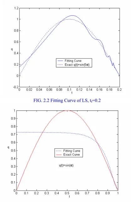
If the exact solution q(t) is known, the coefficients a0 and an may be obtained numericall. Table 1-3 and FIG 2.1-2.3 present the results of sine profiles for tf=0.1, tf=0.2 and tf=1.0, respectively. It appears that series like Eq.(47) do not express well an arbitrary boundary heat flux if the final time is greater than 0.1.

Table 1: Fitting Coefficients of Least Square, Exactq(t)=sin(10πt),t∈[0,0.1]

a0 a1 a2 a3 a4 a5 a6 a7 a8 a9

-0.0004 0.0013 -0.0020 0.0039 -0.0112 0.0392 -0.1354 0.4146 -1.0541 2.1268

a10 a11 a12 a13 a14

-3.2697 3.6541 -2.7738 1.2686 -0.2618

Table 2: Fitting Coefficients of Least Square, Exactq(t)=sin(5πt),t∈[0,0.2]

a0 a1 a2 a3 a4 a5 a6 a7 a8 a9

0.0000 0.0000 0.0000 0.0002 -0.0010 0.0062 -0.0331 0.1464 -0.5196 1.4288

a10 a11 a12 a13 a14

-2.9180 4.1903 -3.9174 2.1011 -0.4839

Table 3: Fitting Coefficients of Least Square, Exactq(t)=sin(πt),t∈[0,1]

a0 a1 a2 a3 a4 a5 a6 a7

0.0007 -0.0008 -0.0033 0.0380 -0.2626 1.1110 -2.2427 1.3598

FIG. 2.2 Fitting Curve of LS, tf=0.2

FIG. 2.3 Fitting Curve of LS, tf=1

Note that the exact heat fluxes q(t)=0.5+eπ2(t−tf)(t

f=1) and q(t)=sin(10πt) (tf=0.1) are recovered with a very good accuracy. For a flux with sine profile (tf=1), the reconstruction solution differs considerably from the exact data, increasing the number of iteration does not improve the results. However this inaccurate solution can make T−TE very small, with a relative error of about 0.01%.

FIG.2.4 Inverse Solution by CGM, Exact heat flux q(t)=0.5+eπ2(t−tf) t

f = 1, ξ=0, S(x,t)=0

FIG.2.6 Inverse Solution by CGM, Exact heat flux q(t)=sin(πt), tf = 1.0, ξ=0, S(x,t)=0

Degree of Ill-Posedness

The degree of ill-posedness is one of the most important character of inverse problems. It influences the stability and accuracy of the inverse (reconstruction) solution. Let us look at the Fredholm integral equation where the decay rate of the singular values wi is an important factor: if it is very fast, the problem is severely ill-posed and vice versa. We may study the ill-posedness of the inverse problem through its kernel [G]. Although the solution is unique, the kernel G strongly depends on the upper limit of the integral, i.e. the final time tf. If the kernel [G] is too “smooth”, the decay rate of its singular values is very fast. FIG.2.7 shows the decay of singular values for different final times. According to the definition of Hofmann [15], a decrease of the final time will decrease the decay rate of singular values. In other words, if the final time is shorter, the inverse problem becomes less ill-posed. This is in agreement with the discrete Picard condition (DPC). The

solution will make the problem ill-posed. From FIG.2.8 and FIG.2.9, we can see that if tf=1, DPC is satisfied only for i<12, and SVD should be truncated at k=11; but if tf=0.1, the truncation parameter k reaches 20. More tests indicate that if tf is longer, k should be smaller, and the problem becomes more ill-posed since a too small truncation parameter will result in the loss of accuracy of solution. Results of a numerical test are presented in FIG.2.10a and b.

If k is chosen by DPC, i.e. k=11, the solution obtained by TSVD is very similar to the one obtained by CGM (see FIG.2.6). However, if k is larger, for example k=13, the DPC will not be satisfied, and the oscillation of solution cannot be avoided.

FIG.2.8 Discrete Picard Condition, Exact solutionq(t)=sin(πt),tf=1, imax=100

FIG.2.10a Solution of Inverse Problem, Exact heat flux q(t)=sin(πt), k=11, imax=100

FIG.2.10b Solution of Inverse Problem, Exact heat flux q(t)=sin(πt), k=13, imax=100

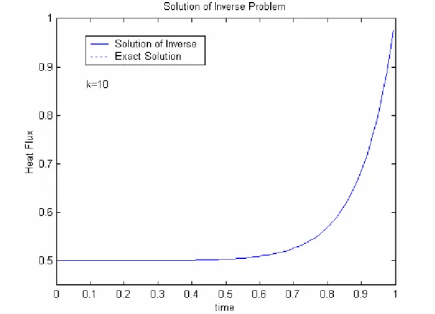
If the final time is short, for example t_f ≤0.1, the problem is moderately or mildly ill-posed. At t_f =0.1, we successfully reconstruct the heat flux with a sine profile. If q(t) may be expressed with Eq. (47), the correct solution can be obtained for any final time. For _{q(t)=0.5+0.5e}t−1.0 _{and t 1}

f = , it is found that the DPC is satisfied for i≤10

FIG.2.11 shows that the inverse solution agrees perfectly with the exact data. It can be concluded that the IHCP of second kind can be regularized successfully for any final time if q(t) has a profile of Eq.(47).

FIG. 2.11 Inverse Solution by TSVD, Exact heat flux _{q(t)=0.5+0.5e}t−1.0_{, t}

f=1.0, k=10, imax=100

Modified CGM

The above results show that the inverse solution is very difficult to converge to the exact value if the final time is greater than 0.1. On other hand, the global minimum (namely the heat flux q that makes the error functional E(q) exactly equal to zero) is unique. A proper search direction we may lead to the global minimum. In fact, a modification of the conjugate direction is found to improve the reconstruction results. This modified CG method [16-19] is based on the assumption that q(t) is a continuously differentiable function defined as

) t ( q d ) t ( dq t t _{′ ∆ ′}

q(t=0)=∆q(t=0)=0 (48) Applying the rule of differentiation under the integral sign, we have the identity

) t , 1 ( T t d ) t , 1 ( T dt d t tf = ′ ′

∫

(49) Introducing Eq.(53) into Eq.(15), we obtain

dt q t d ) t , 1 ( T dt d ) q ( E D dt dq E D f f t 0 t t q q

∫

∫

        ∆ ⋅         ′ ′ = ≡       ∆ ∆ (50)

Integrating the first term of the right hand side of Eq. (50) by parts and rewriting the second term, we get

∫

∫

∫

_       ′ ′ ∆ −         ∆ ⋅         ′ ′ =       ∆ f f f f t 0 t t t 0 t t q T(1,t)dt dt dt q d q t d ) t , 1 ( T dt dq E D (51) Then

∫

∫

_       ′ ′ − ∆ =       ∆ f f t 0 t t q T(1,t)dt dt dt q d dt dq E D (52)

By comparing Eq.(9) with Eq.(52), we have

∫

∫

′ ∇ = ′ ′ − =       ∇ f f t t t t t Ed t d ) t , 1 ( T dt dq E (53)

The modified search direction is related to the derivative of the direction of decent Rk _{by the relation} =

_∫

t ′ 0 k k _{R dt} p (54) where k k_Rk 1 dt dq E R +γ −      −∇ = (55) and the conjugate coefficient _γk _{is given by Eq. (18) and the gradient of the error}

function is       ∆ ∇ dt q d E :

∫

∫

⋅             ∇ ⋅       ∇ ⋅             ∇ −       ∇ = γ − − f f t 0 2 1 k t 0 k 1 k k k dx dt dq E dx dt dq E dt dq E dt dq E (56)

If we make a modification according to Eq.(54), the search direction becomes

∑

∞

(

)

= π − − π     ₋ π − π + + = 1 n t n ) t t ( n 2 2 2 2 n 2 02 01 k mod f 2 2 f 2 2 e e n 1 t n c t c t c ) t ( p (57)

which contains linear and second order components and is thus more adaptable to an arbitrary heat flux than the regular search direction. However, its shortcoming is

guess initial ) 0 t ( pk

mod = = , i.e. the inverse solution is equal to the initial guess at t=0.

Our strategy is therefore:

1) set initial guess=0, solve the minimization problem using the modified method firstly;

2) set the solution of 1) as initial guess, solve the minimization problem using regular method and obtain the final inverse solution.

Numerical Solutions by CGM and TSVD

Typical Profiles

In this section, we reconstruct some typical profiles during the time interval

1 . 0 t

0≤ ≤ . Linear and sine curves are well recovered by CGM and TSVD (see FIG.2.5, FIG.3.1). However, the iterative CGM may need hundreds of iterations to arrive at an accurate solution. The process of convergence is slow, and computation time is long. TSVD is a direct regularization method and its total calculation time is much shorter. The inverse solutions for the triangular profile are acceptable. Comparing the solutions obtained by TSVD with the solutions obtained by CGM, we remark that the former are better than the latter. It may be due to the fact that the accumulation of numerical errors in the iteration process may affect the accuracy of solutions. As for long pulse heating which is often used in industries, the result is reasonable but its accuracy is not satisfactory as a smooth heat flux q(t) is easier

FIG.3.1a Inverse Solution by CGM, Exact heat flux q(t)=10t, tf = 0.1, ξ=0, S(x,t)=0

FIG.3.1b Inverse Solution by TSVD, Exact heat flux q(t)=10t, tf = 0.1, k=20, S(x,t)=0

FIG.3.2b Inverse Solution by TSVD, Triangular exact heat flux profile, tf =0.1, k=20, S(x,t)=0

Inverse Solutions with Noisy Data

In practice, the errors of measurements cannot be avoided. In order to simulate the actual measurements, the noisy data T_E(1+σ∑) are used instead of the exact data TE, where Σ <1 is a uniformly distributed random real number. In

ill-posed problems, a small error in input data may result in a big error in the solution. FIG.3.4 shows that a small error (σ=0.001) can affect the Picard condition

significantly. Tikhonov method can be used in both CGM and SVD methods to regularize the solution. Determining the regularization parameter is the most important task in Tikhonov method. A well-known method of choosing the regularization parameter is the L-curve criterion [20]. This method proposes that the optimal regularization parameter that balances the regularization errors and perturbation errors occurs at the “corner” of a plot of solution norm vs. residual norm.

FIG.3.4a Discrete Picard Condition Exact solution q(t)₌exp[_π2(t₋t_f)]

tf=1.0, σ=0, imax=100

FIG.3.4b Discrete Picard Condition Exact solution q(t)₌exp[_π2(t₋t_f)]

tf=1.0, σ=0.001, imax=100

In this report we only determine ξ for SVD method, because the whole process is

the same for CGM, it should be only remarked that the optimal regularization parameters for CGM and for SVD may be different. Normally, the latter is greater than the former because CGM has a stronger regularization ability. FIG.3.5 gives an example of L-curve for SVD algorithm, for an exact heat flux q(t)=10t, with a

final time tf=0.1 and a noise level σ=0.01. The vertical axis denotes the residual norm Gq−TE ₂; the horizontal axis denotes the norm of the regularized solution q ₂.

For each ξ, we get a point. For a set of ξ, we get an L-shaped curve. The “corner”

point ξ=0.001 is the optimal regularization parameter. The corresponding regularized solution shown in FIG.3.6 is very close to the exact solution. If ξ is

more or less than this value, the reconstructed solution will oscillate or bias the true heat flux. The results of another test (see FIG.3.7 and FIG.3.8) suggest that if the heat flux is of the form given by Eq. (47), the inverse solution is not significantly affected by random noises even with σ as large as 10%. SVD and CGM

provide similar solutions even though their regularization parameters are different.

FIG.3.6 Inverse Solution by SVD, Exact solution q(t)=10t, Noise level σ=0.01, ξ=0.001

FIG. 3.7 Inverse Solution by CGM FIG.3.8 Inverse Solution by SVD Exact heat flux q(t)₌exp[_π2(t₋t_f)] _{Exact heat flux q(t) exp[ (t t )]}

f 2 ₋ π = 1 . 0 = σ , 001ξ=0. σ=0.1, 01ξ=0.

FIG.3.9 Inverse Solution for Unconstrained Problem

FIG.3.10 Inverse Solution for Constrained Problem

Constrained and Unconstrained Control Problems

Let us consider the following control problem: the temperature is zero at t=0, determine the heat flux at active boundary to obtain a temperature as uniform as possible at tf=1, e.g. T(x,1)=1. The exact solution for this problem does not exist and the ‘optimum’ solution is not unique. In engineering practice, the heating process may be limited by several conditions, and we have to deal with a constrained control problem. For example, the constraints on the boundary heat flux may be q_min(t) =0,q_max(t)=0.1+4t . The solutions for the unconstrained and constrained problems are illustrated in Fig.3.9 and Fig.3.10. For the former, the

Numerical Solutions by Modified CGM

Some Typical Profiles

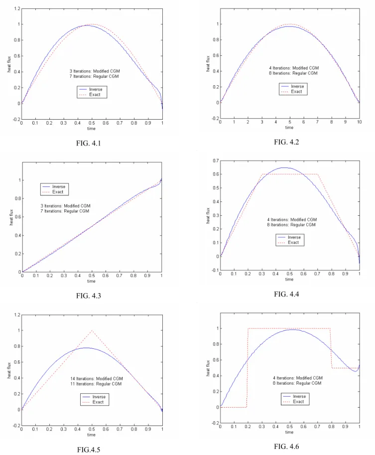
In this section, we reconstruct of some typical profiles. Linear and sine curves are well recovered by a combination of the modified and regular CGM (see FIG.4.1-FIG.4.3). We start the iteration process with the modified CGM until a reasonable profile of heat flux is attained. Afterwards, the regular CGM is employed to accelerate the convergence. The estimation by the modified CGM is treated as the initial guess values. Comparing FIG4.1 with FIG.4.2, we may conclude that the accuracy of the solution is not affected by the final time. The inverse solutions shown in FIG.4.4 and FIG.4.5 with the triangular and trapezoidal profiles are acceptable. As for rectangular or stair-shaped profiles which are often used in industries, the results (FIG.4.6) are reasonable but their accuracies are not satisfactory.

Inverse Solutions with Noisy Data

In order to simulate the errors in actual measurements, data with relative errors

) 1 (

T_E +σ∑ or with absolute errors T_E +T_maxσ∑are used instead of the exact value T_E,

where Σ <1 is a uniformly distributed random real number and Tmaxis the maximum

range of the measurement device. Although Tikhonov regularization may stabilize the solution effectively, the CGM itself also has a regularization power, and Tikhonov regularization is not always necessary in CGM. In this section, the Tikhonov parameter is set to zero.

The numerical tests indicate that a maximum relative error of 5% and a maximum absolute error of 0.05⋅Tmax (class 5 accuracy) do not affect the accuracy of the

FIG. 4.1 FIG. 4.3 FIG.4.5 FIG. 4.2 FIG. 4.4 FIG. 4.6

Modified CGM is based on the assumption q(t)=∆q(t =0)=0which makes the search direction Pk(t₌0)₌0_{. If the exact q(t=0) is not equal to this initial guess value, the} additional iterations executed by using regular CGM does not help (FIG.4.10.1) because this method cannot find the correct solutions near the initial time. However, if q(t=0) is known, this difficulty may be alleviated by setting it as the initial guess (FIG.4.10.2). In engineering practice, the exact heat flux at t=0 is not known, but a possible range may be given. FIG.4.10.3 and FIG.4.10.4 show that an acceptable solution can be obtained even with an error of ±20% in the initial guess. Optimal Control Problem

Let us determine the heat flux at the active boundary to obtain a temperature as uniform as possible at tf=1, e.g. T(x,1)=1. The solutions obtained by the regular and modified CGM are respectively illustrated in Fig.4.11 and Fig.4.12. For the former, the relative error Er= T−TE /TE is about 0.91% after 9

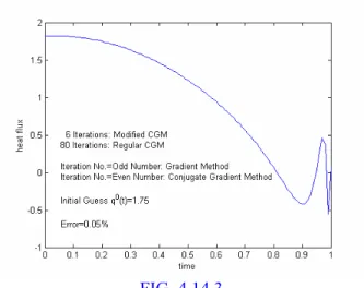
iterations; for the latter, E_r =0.51%.This suggests that the modified method gives a better solution. To achieve a uniform temperature at the final time, the heat flux at the beginning of heating process should be as high as possible. Suppose the maximum possible heat flux qmax=1.75, and set it as the initial guess, the modified CGM may give a solution with a relative error of 0.28% as shown in FIG.4.13.

FIG.4.7.1: Inverse Solution

FIG.4.8.1: Inverse Solution

FIG.4.9.1: Inverse Solution

FIG.4.7.2: Relative Error σ=5%

FIG.4.8.2: Relative Error σ=5%

FIG.4.9.2: Absolute Error

05 . 0 =

FIG.4.10.1

FIG.4.10.3

FIG.4.10.2

FIG.4.10.4

FIG. 4.12

FIG. 4.13

Alternating Searching Direction

We note that the convergence may be very difficult after 9 iterations if the final time is equal to 1.0. The relative error will not decrease as the iteration number is increased. If we alternate the search directions, e.g. gradient direction (steepest descent method) and conjugate gradient direction, we may obtain a better solution as shown in FIG.4.14. As the solution of this optimization problem is not unique, the alternating search direction technique may avoid some “bad” points

Optimal Heating Time

If the heating process is longer, the final temperature distribution is more uniform. If the final time is infinite, the temperature distribution may be absolutely uniform! Industrial heating requires however a heating time as short as possible to achieve a high production rate. FIG.4.15 presents the relationship between the final time and the relative error. The corner of the L-shaped curve is the optimum point. For regular CGM or modified CGM, the optimum final time is 0.5. The heating strategies for tf=0.5 are shown in FIG.4.16 and FIG.4.17. The evolutions of the temperature distributions for tf=0.5 and tf=1.0 are illustrated in FIG.4.18 and FIG.4.19. Unfortunately, such an optimal heating yields

(

Tmax −TE

)

/TE over 55% if

tf=0.5 !

A Real Industrial Example

Let us consider the heating process of an aluminum billet with a diameter of 76mm from 20 to 580 o_{C in 300 seconds, such that the final temperature should} be as uniform as possible. The dimensionless time corresponding to 5 minutes is 10. Both regular CGM and modified CGM may lead to an optimal heating strategy (FIG.4.20 and FIG.4.21). However, the latter scheme is easier realize than the former because it is smoother and requires no cooling period.

FIG.4.16 FIG. 4.14.2 0 1 2 3 4 5 6 7 8 0 0.2 0.4 0.6 0.8 1 1.2 1.4 1.6 1.8 2 Time R el at iv e E rro r (% ) Regular CGM Modified CGM+Regular CGM FIG. 4.15 FIG. 4.17 FIG.4.18.1 FIG.4.19.1

FIG.4.18.2 FIG.4.19.2

FIG.4.20.1

FIG.4.21.1

FIG.4.20.2

Conclusion

Singular value decomposition and iterative conjugate gradient methods are used to solve the IHCP of second kind. It is found that this inverse problem is severely ill-posed. In general, it is possible to recover a boundary heat flux only for a non-dimensional final time of the order of 0.1. On the other hand, for control problems, either constrained or unconstrained, we can obtain a satisfactory solution with a very small discrepancy between the target and the actual temperatures at the final time.

A modified conjugate gradient method may be used to reconstruct a heat flux with satisfactory accuracy for any final time if its value at t=0 is known. For boundary control problems, the modified algorithm may give a better solution than the CGM. Acknowledgements

This research was supported by the Natural Sciences and Engineering Research Council of Canada.

REFERENCES

1. A.N. Tikhonov, Regularization of Ill-posed Problems, Doklady Akad. Nauk SSSR, Vol.153, 1963.

2. O.M. Alifanov, Inverse Heat Transfer Problems, Springer-Verlag, Berlin Heidelberg, 1994.

3. J.V. Beck, B. Blackwell, C.R. St-Clair Jr, Inverse Heat Conduction: Ill-Posed Problems, Wiley Interscience, New York, 1985.

4. D. A. Murio, The Mollification Method and the Numerical Solution of Ill-Posed Problems, John Wiley & Sons, New York, 1993.

Packaging and Manufacturing Technology (CPMT)-Part A, Vol. 18, No.3, pp. 540-545, 1995.

6. K.A. Woodbury, Inverse Engineering Handbook, CRC Press, Boca Raton, 2003. 7. T.H. Nguyen, X.L. Zhang, Back to the Initial State of Convection: A Retrospective Heat Transfer Problem, 1994

8. R. Lezius and F. Tröltzsch, Theoretical and Numerical Aspects of Controlled Cooling of Steel Profiles, Progress in Industrial Mathematics at ECMI 94, Wiley-Tenbner, pp. 380-388, 1996.

9. T.H. Nguyen, C-Q. Zheng, C.A Loong, Induction Heating of Semi-Solid Aluminum and Magnesium Alloys, 2nd Internation Conference on Computational Heat and Mass Transfer, Rio de Janeiro, Brazil, October 2001.

10. Hsin-Sen Chu, Temperature uniformity of 12-inch silicon wafer during rapid thermal processing, Journal of the Chinese Society of Mechanical Engineers, Vol. 24, No. 4, pp.391-406, 2003.

11. C.T. Kelley and E. W. Sachs, A Trust Region Method for Parabolic Boundary Control Problems, SIAM J. Optimization., Vol.9, No.4, pp. 1064-1081, 1999.

12. C.H. Huang, A Nonlinear Optimal Control Problem in Determining the Strength of the Optimal Boundary Heat Fluxes, Numerical Heat Transfer, Part B, Vol.40, pp.411-429, 2001.

13. C.H. Huang and C.Y. Li, A Three-Dimensional Optimal Control Problem in Determining the Boundary Control Heat Fluxes, Heat and Mass Transfer, Vol.39, pp. 589-598, 2003.

14. M. H. James and N. D. Dewynne, Heat Conduction, Blackwell Science Publications, Oxford London Edinburgh, 1986.

15. B. Hofmann, Regularization for Applied Inverse and Ill-Posed Problems, Teubner, Stuttgart, German, 1986.

16. C.H. Huang and M.N. Özisik, Inverse Problem of Determining Unknown Wall Heat Flux in Laminar Flow Through a Parallel Plate Duct, Numerical Heat Transfer, Part A, 21, pp.55-70 ,1992.

17. H. M. Park and O. Y. Chung, An Inverse Natural Convection Problem of Estimating the Strength of a Heat Source, Int. J. Heat Mass Transfer, 42, pp. 4259-4273, 1999.

18. H.M. Park and W.S. Jung, The Karhunen-Loève Galerkin Method for the Inverse Natural Convection Problems, Int. J. Heat Mass Transfer, 44, pp. 155-167 , 2001.

19. S. Jasmin and M. Prud´homme, Inverse determination of a heat source from a solute concentration generation model in porous medium, Int. J. Heat Mass Transfer, 2004.

20. P.C. Hanson, Rank-Deficient and Discrete Ill-Posed Problems: Numerical Aspects of Linear Inversion, SIAM, Philadelphia, 1998.