WASP-166b: a bloated super-Neptune transiting a V = 9 star

arXiv:1811.05292v2 [astro-ph.EP] 9 Jul 2019

WASP-166b: a bloated super-Neptune transiting a V = 9

star

Coel Hellier

1

, D.R. Anderson

1

, A.H.M.J. Triaud

2,3

, F. Bouchy

2

, A. Burdanov

4

,

A. Collier Cameron

5

, L. Delrez

4,6

, D. Ehrenreich

2

, M. Gillon

4

, E. Jehin

4

,

M. Lendl

7,2

, E. Linder

8

, L.D. Nielsen

2

, P.F.L. Maxted

1

, F. Pepe

2

, D. Pollacco

9

,

D. Queloz

6

, D. S´egransan

2

, B. Smalley

1

, J. J. Spake

10

, L. Y. Temple

1

, S. Udry

2

,

R.G. West

9

, and A. Wyttenbach

11

1_{Astrophysics Group, Keele University, Staffordshire, ST5 5BG, UK}

2_{Observatoire astronomique de l’Universit´e de Gen`eve 51 ch. des Maillettes, 1290 Sauverny, Switzerland</sub> 3<sub>School of Physics & Astronomy, University of Birmingham, Edgbaston, Birmingham, B15 2TT, UK</sub> 4<sub>Space sciences, Technologies and Astrophysics Research (STAR) Institute, Universit´e de Li`ege,} All´ee du 6 Aoˆut, 17, Bat. B5C, 4000 Li`ege, Belgium

5_{SUPA, School of Physics and Astronomy, University of St. Andrews, North Haugh, Fife, KY16 9SS, UK} 6_{Cavendish Laboratory, J J Thomson Avenue, Cambridge, CB3 0HE, UK}

7_{Space Research Institute, Austrian Academy of Sciences, Schmiedlstr. 6, 8042, Graz, Austria} 8_{Physikalisches Institut, University of Bern, Sidlerstrasse 5, 3012, Bern, Switzerland}

9_{Department of Physics, University of Warwick, Gibbet Hill Road, Coventry CV4 7AL, UK} 10_{Astrophysics Group, School of Physics, University of Exeter, Stocker Road, Exeter, EX4 4QL, UK} 11_{Leiden Observatory, Leiden University, Postbus 9513, 2300 RA Leiden, The Netherlands}

date

ABSTRACT

We report the discovery of WASP-166b, a super-Neptune planet with a mass of 0.1

M

(1.9 M

) and a bloated radius of 0.63 R

. It transits a V = 9.36, F9V star

in a 5.44-d orbit that is aligned with the stellar rotation axis (sky-projected obliquity

angle λ = 3 ± 5 degrees). Variations in the radial-velocity measurements are likely the

result of magnetic activity over a 12-d stellar rotation period. WASP-166b appears to

be a rare object within the “Neptune desert”.

Key words:

Planetary Systems – stars: individual (WASP-166)

1

INTRODUCTION

Planets with low surface gravities have the largest

atmo-spheric scale heights and so are the best targets for

at-mospheric characterisation by the technique of transmission

spectroscopy, in which the planet’s atmosphere is projected

against the host-star photosphere during transit. Having a

bloated radius also means that planets of sub-Saturn mass

can still produce deep-enough transits to be found in

ground-based surveys. Thus discoveries such as WASP-107b (0.12

M

; 0.94 R

;

Anderson et al. 2017

) and WASP-127b

(0.18 M

; 1.37 R

;

Lam et al. 2017

) are prime targets

for characterisation (e.g.

Kreidberg et al. 2018

;

Spake et al.

2018

;

Palle et al. 2017

;

Chen et al. 2018

). The importance

of such targets, particularly ones transiting bright stars, will

increase further with the launch of the James Webb Space

Telescope.

Planets between the masses of Neptune and Saturn are

transitional between ice giants and gaseous giants, and so

could help to elucidate why some proto-planets undergo

run-away gaseous accretion while others do not. There are also

far fewer Neptune-mass systems known, compared to the

abundance of super-Earths found by the Kepler mission,

and the several-hundred transiting hot Jupiters now found

by the ground-based surveys. The absence of Neptunes is

particularly pronounced at short orbital periods, leading to

the discussion of a “Neptune desert” (

Mazeh et al. 2016

).

Here we report the discovery of WASP-166b, the

lowest-mass planet yet found by the WASP survey, at only twice

the mass of Neptune.

2

OBSERVATIONS

From 2006 to 2012 WASP-South operated as an array of

eight cameras based on 200-mm, f/1.8 Canon lenses backed

by 2k×2k Peltier-cooled CCDs (see

Pollacco et al. 2006

for

an account of the WASP project). Each field was observed

Relative flux WASP 0.99 1 1.01 0.4 0.6 0.8 1 1.2 1.4 1.6 Relative flux Orbital phase TRAPPIST EulerCAM TESS 0.97 0.98 0.99 1 0.98 1 1.02

Figure 1. WASP-166b photometry: (Top) The WASP data folded on the transit period. (Main panel) Photometry from TRAPPIST-South, EulerCAM, and the three TESS transits, to-gether with the fitted MCMC model (the TRAPPIST ingress, green points, and egress, blue points, are from different transits but are shown together).

with typically 10-min cadence. The data were processed

into a magnitude for each catalogued star, and the

result-ing lightcurves accumulated in a central archive. This was

then searched for transit signals, with the best candidates

sent for followup with the TRAPPIST-South photometer

(

Gillon et al. 2013

) and the Euler/CORALIE spectrograph

(

Triaud et al. 2013

). This combination has resulted in many

discoveries of transiting exoplanets (e.g.

Hellier et al. 2018

)

and the techniques and methods used here are continuations

of those from previous papers.

WASP-166 was adopted as a candidate in 2014, after

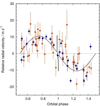
Relative radial velocity / m s

-1 Orbital phase -20 -10 0 10 20 30 0.6 0.8 1 1.2 1.4

Figure 2.The HARPS (blue) and CORALIE (orange) radial velocities and fitted orbital model (the HARPS data in Fig. 4 are not shown here for clarity).

Table 1.Observations of WASP-166:

Facility Date Notes

WASP-South 2006 May–2012 May 33 400 points

CORALIE 2014 Feb–2017 Jan 41 RVs

HARPS (orbit) 2016 Apr–2018 Mar 27 RVs HARPS (transit) 2017 Jan 14 75 RVs HARPS (transit) 2017 Mar 04 52 RVs HARPS (transit) 2017 Mar 15 66 RVs

TRAPPIST-South 2014 Mar 05 z band

EulerCAM 2016 Feb 05 Icband

TRAPPIST-South 2016 Feb 16 z′_band

TESS 2019 Feb 2–27 3 transits

detection of a 5.44-d transit signal. Radial-velocity (RV)

observations with CORALIE found orbital motion at the

transit period, but also showed additional variations. We

thus accumulated more RV data than is usual for WASP

planet discoveries in order to look for additional bodies or

a longer-term trend. This amounted to 41 RVs with

1.2-m Euler/CORALIE over a three-year period, and 220 RVs

with the ESO 3.6-m/HARPS, of which 27 covered the orbit,

while 75, 52 and 66 were taken in sequences covering

tran-sits on three different nights. The CORALIE and HARPS

data were reduced using standard pipelines, as described

in

Rickman et al.

(

2019

),

Udry et al.

(

2019

) and references

therein.

Further photometric observations (listed in Table 1)

in-clude two partial transit lightcurves from TRAPPIST-South

(one ingress and one egress) and a full transit from

Euler-CAM (

Lendl et al. 2012

), which unfortunately has excess

red noise owing to poor observing conditions.

In 2019 February, after completion of the initial version

of this paper, the TESS satellite observed the sky sector

Bisector span / m s -1

HARPS

CORALIE

Figure 3.The spectroscopic bisector spans against orbital phase. The HARPS and CORALIE data are plotted separately since their accuracy is different. The absence of any correlation with radial velocity is a check against transit mimics.

Relative radial velocity / m s

-1 Orbital phase -35 -30 -25 -20 -15 -10 -5 0 5 10 15 20 25 0.96 0.97 0.98 0.99 1 1.01 1.02 1.03 1.04

Figure 4.HARPS radial-velocity data through transit along with the fitted R–M model. The colours denote data from different nights (blue: 2017-01-14; green 2017-03-04; orange 2017-03-15).

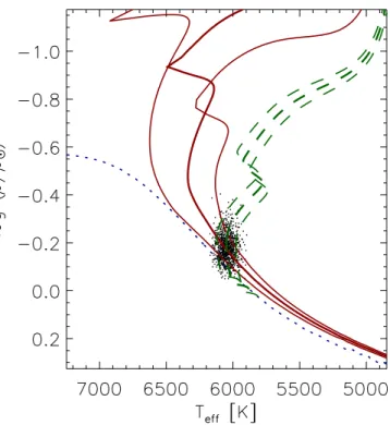
Figure 5. The host star’s effective temperature (Teff) versus density (where the dots are outputs of the bagemass MCMC). The blue dotted line is the zero-age main sequence, the green dashed lines are the evolutionary tracks (for the best-fitting mass of 1.18 M⊙and error bounds of 0.03 M⊙), while the red lines are isochrones (for the best-fitting age of 2.1 Gyr and error bars of 0.9 Gyr).

that includes WASP-166. TESS (

Ricker et al. 2016

) is

per-forming an all-sky transit survey aimed primarily at rocky

planets too small to be found by the ground-based surveys.

It has four cameras, each with a 10-cm lens backed by four

2048x2048 CCDs covering a field of 24

_x24

_{, and observing}

in a bandpass from 600 to 1000 nm.

We downloaded the public TESS lightcurve for

WASP-166 (= TIC 408310006 = TOI-576) from the Mikulski

Archive for Space Telescopes (MAST). We used the

stan-dard aperture-photometry data products, and extracted

sec-tions of the data around the known transit times. Three

transits were observed over the 25-d period (a fourth was

recorded shortly after recovery from a data gap, and we

dis-card it owing to strong out-of-transit variability).

3

SPECTRAL ANALYSIS

For a spectral analysis of the host star we combined and

added the HARPS spectra and adopted the methods of

Doyle et al.

(

2013

). The resulting parameters are listed in

Table 2. The effective temperature, T

= 6050 ± 50 K,

comes from the Hα line, and suggests a spectral type of F9.

The surface gravity, log g = 4.5 ± 0.1 comes from Na i D

and Mg i b lines. The metallicity value of [Fe/H] = +0.19

±

_{0.05 comes from equivalent-width measurements of}

un-blended Fe i lines. The Fe i lines were also used to estimate

Table 2.System parameters for WASP-166. 1SWASP J093930.08–205856.8 2MASS 09393009–2058568 BD–20 2976 RA = 09h₃₉m_30.09s_{, Dec = –20}◦₅₈′ 56.9′′ (J2000) V mag = 9.36; GAIA G = 9.26; J = 8.35 Rotational modulation: < 1 mmag

GAIA DR2 pm (RA) –55.082 ± 0.072 (Dec) 10.927 ± 0.069 mas/yr GAIA DR2 parallax: 8.7301 ± 0.0448 mas

Distance = 113 ± 1 pc

Stellar parameters from spectroscopic analysis.

Spectral type F9V Teff (K) 6050 ± 50 log g 4.5 ± 0.1 v sin i (km s−1_{) 4.6 ± 0.8} [Fe/H] +0.19 ± 0.05 log A(Li) 2.68 ± 0.08

Age (bagemass) (Gyr) 2.1 ± 0.9

Parameters from MCMC analysis (fitted parameters denoted †).

P (d)† _{5.443540 ± 0.000004} Tc(TDB)† _{245 7664.3289 ± 0.0006} T14(d)† _{0.150 ± 0.001} T12= T34(d) 0.0088 ± 0.0012 ∆F†_{= R}2 P/R2∗ 0.00281 ± 0.00007 b† _{0.39 ± 0.10} i (◦_{) 88.0 ± 0.7} K1(km s−1₎† _{0.0104 ± 0.0004} γ (km s−1₎† _{23.6285 ± 0.0003} e 0 (adopted) (< 0.07 at 2σ) a/R∗ 11.3 ± 0.6 M∗(M⊙) 1.19 ± 0.06 R∗(R⊙) 1.22 ± 0.06 log g∗(cgs) 4.34 ± 0.05 ρ∗(ρ⊙) 0.65 ± 0.10 MP (MJup) 0.101 ± 0.005 RP(RJup) 0.63 ± 0.03 log gP(cgs) 2.77 ± 0.05 ρP(ρJ) 0.41 ± 0.07 λ (deg)† _{3 ± 5} v sin i (km s−1_{) 5.1 ± 0.3} a (AU) 0.0641 ± 0.0011 Irradiation (W m−2_{) 6.0 ± 0.6 ×10}5 TP,A=0(K) 1270 ± 30

Priors were M∗= 1.18 ± 0.03 M⊙and R∗= 1.23 ± 0.06 R⊙ Errors are 1σ; Limb-darkening coefficients were:

r band: a1 = 0.512, a2 = 0.337, a3 = –0.138, a4 = –0.015 I band: a1 = 0.579, a2 = 0.039, a3 = 0.104, a4 = –0.101 z band: a1 = 0.599 , a2 = –0.076 , a3 = 0.191, a4 = –0.131

a rotation speed of v sin i = 4.6 ± 0.8 km s

_{, after}

convolv-ing with the HARPS instrumental resolution (R = 120 000),

and also accounting for an estimate of the macroturbulence

take from

Doyle et al.

(

2014

). We also report a value for the

lithium abundance of log A(Li) = 2.68 ± 0.08.

According to Gaia DR2 (

Gaia Collaboration et al.

2018

), WASP-166 has a relatively high proper motion of

56 mas/yr, which at the DR2 distance gives a transverse

velocity of 30.0 ± 0.3 km s

_{, which complements the DR2}

radial velocity of 24.0 ± 0.4 km s

_{. WASP-166 is relatively}

isolated, with the nearest DR2 star being 8 arcsecs away and

9 magnitudes fainter. There is no excess astrometric noise

reported (such noise can indicate an unresolved binary).

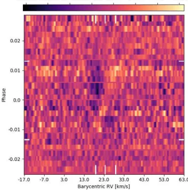
Figure 6.The line profiles through transit. The white lines show (x-axis) the mean γ velocity of the system and the v sin i line width, and (y-axis) the beginning and end of transit. The Doppler shadow of the planet moves from blue to red over the transit. The mean profile has been subtracted, resulting in a reduced level elsewhere in transit.

4

SYSTEM ANALYSIS

As is standard for WASP discovery papers, we combined the

photometry and radial-velocity datasets into a Markov-chain

Monte-Carlo (MCMC) analysis (e.g.

Collier Cameron et al.

2007

). This fits parameters including T

(the epoch of

mid-transit), P (the orbital period), ∆F (the transit depth that

would be observed in the absence of limb-darkening), T

(duration from first to fourth contact), b (the impact

pa-rameter) and K

(the stellar reflex velocity). For fitting the

photometry we adopted the 4-parameter, non-linear limb

darkening of

Claret

(

2000

), interpolating coefficients for the

appropriate stellar temperature and metallicity.

We allowed for radial-velocity offsets between different

datasets, treating the CORALIE data before and after a

November 2014 upgrade, the HARPS data round the orbit,

and the three HARPS transit observations, all as

indepen-dent sets (the RV values are listed in Table A1). The γ

velocity of the system given in Table 2 is that for the 27

HARPS datapoints around the orbit.

We adopted a zero-eccentricity fit for WASP-166b, as

is usually the case for lower-mass, short-period planets. It is

clear, though, that there are additional radial-velocity

devi-ations from the fitted model; indeed the fit to the HARPS

RVs around the orbit has a χ

_{of 217 for 27 datapoints.}

Allowing an eccentric solution did not significantly improve

the fit (producing a not-significant value of e = 0.03 ± 0.02,

with a 2-σ upper limit of 0.07), nor did allowing a

long-term drift in the RVs. Adding a second sinusoid, as could

be caused by a second planet, also failed to model the

ad-ditional variability, with tells us that it is not a coherent

modulation.

The MCMC process accounts for the additional RV

variability, and indeed any red noise in the transit

lightcurves, by inflating each dataset’s errors to give χ

ν

= 1;

this balances the different datasets’ influence on the final

re-sult and inflates the errors on the output parameters.

As is usual in WASP discovery papers we also

con-strained the stellar mass by adopting a prior based on the

measured effective temperature and metallicity values,

to-gether with the stellar density obtained by an initial fit to

the transit. For this we used the bagemass code described

in

Maxted et al.

(

2015

). This resulted in a mass estimate of

1.18 ± 0.03 M

, and also an age estimate of 2.1 ± 0.9 Gyr.

The measured lithium abundance is consistent with this age

estimate, though does not constrain the age further.

Lastly, we include a constraint on the stellar radius

de-rived from Gaia DR2 (

Gaia Collaboration et al. 2018

). The

DR2 parallax of 8.730 ± 0.045 mas implies a distance of 113

±

_{1 pc (where we have applied the correction suggested by}

Stassun & Torres 2018

). Using the Infra-Red Flux Method

(

Blackwell & Shallis 1977

) this implies a stellar radius of

1.23 ± 0.06 R

, which we adopt as a prior. The initial

ver-sion of this paper lacked the TESS data and so, with only

limited photometry, the parameters were less secure.

How-ever, the Gaia input tied down the stellar radius, and hence

the impact parameter, and thus, after including the TESS

data, the values have changed by less than an error bar.

The adopted system parameters are listed in Table 2,

while the data and fit are shown in Figs. 1 to 4. We also

show a modified H–R diagram for the star in Fig.

5

.

4.1

The Rossiter–McLaughlin effect

The above MCMC fit included fitting the in-transit

ra-dial velocities, where we use the parameterisation of

Hirano et al.

(

2011

) to model the RV deviations caused by

the Rossiter–McLaughlin effect (Fig. 4). Any differences

be-tween the data on the three different nights of data could be

caused by the planet crossing starspots or faculae regions.

The sky-projected obliquity angle, λ, is measured as

3 ± 5 degrees, and thus the planet’s orbit is aligned with

the stellar rotation. The fitted v sin i of 5.1 ± 0.3 km s

_is

consistent with the spectroscopic value of 4.6 ± 0.8 km s

_.

In Fig. 6 we show the HARPS line profiles through

transit, in a tomographic display following the methods in

Temple et al.

(

2018

). This figure shows the averaged data

from all three transits, with the mean profile subtracted to

better show variations. The planet trace can be seen moving

prograde from blue to red over the transit. Fitting the

to-mogram directly (e.g.

Temple et al. 2018

), as opposed to

fit-ting the modelled RVs, produces parameters consistent with

those in Table 2, where again the uncertainties are currently

dominated by the quality of the photometry.

4.2

Possible magnetic activity

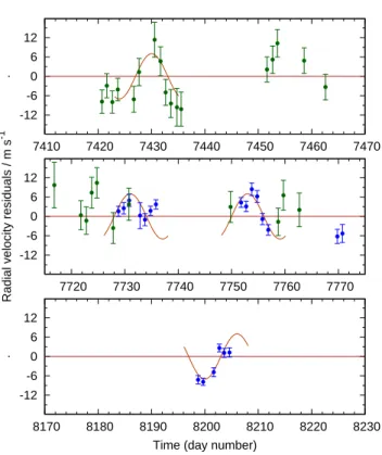
The RV data clearly show deviations about the orbital model

(Fig. 2). To illustrate this we plot in Fig. 7 some of the

resid-ual RV values as a function of time (omitting the in-transit

R–M sequences). The residuals appear to be correlated from

night to night.

Radial velocity residuals / m s

-1 -12 -6 0 6 12 8170 8180 8190 8200 8210 8220 8230 .

Time (day number)

Figure 7. The residuals of the RV data to the orbital model, plotted as a function of time. Blue and green symbols are HARPS and CORALIE data respectively. The red line shows portions of sinusoid (not phase coherent) that illustrate the putative 12.1-day stellar rotation period.

Given the transit and the fact that the planet’s orbit

is aligned we can presume that the stellar rotation axis is

perpendicular to the line of sight, and thus combining the

v

sin i fitted to the R–M effect with the fitted stellar radius

we obtain a rotational period of 12.1 ± 0.9 days. To guide the

eye we plot in Fig. 7 portions of 12.1-d sinusoid (amplitude

7 m s

_{), and conclude that the RV deviations might result}

from magnetic activity.

We have also investigated the variability by modelling

the HARPS RVs using a gaussian-process (GP) analysis

fol-lowing the method detailed in

Haywood et al.

(

2014

). To

model the residuals, this adds to the orbital motion three

hyperparameters (with uniform priors), namely an

ampli-tude a, a period P

(taken to be the rotational period), and

an exponential decay timescale, t

(being the timescale

on which magnetic activity would lose coherence). We set

the last to ∼ 30 d, which is physically realistic, but is not

constrained by the data since we have few observations

sepa-rated by that timescale. The “corner plot” of the GP output

is shown in Fig. 8.

The analysis produces a clear preference for a rotational

period of 12.3 ± 1.9 days, consistent with that from the R–

M v sin i, and in line with the magnetic-activity hypothesis.

The resulting values of K

= 0.0100 ± 0.0006 km s

and

γ

= 23.6288 ± 0.0012 km s

_{are consistent with those in}

Table 2.

Having found evidence of a 12-d rotational period we

then searched the WASP lightcurve for any rotational

mod-0.0000 06 0.0000 12 0.0000 18 0.0000 24 a 7.5 10.0 12.5 15.0 17.5 Prot (d ay ) 24 28 32 36 40 tdeca y (d ay ) 0.00880.00960.01040.0112 K (km~s−1) 23.626 23.628 23.630 23.632 γ (km ~s −1) 0.0000 06 0.0000 12 0.0000 18 0.0000 24 a 7.5 10.0 12.5 15.0 17.5 Prot (day) 24 28 32 36 40 tdecay (day) 23.6 26 23.62823.63023.632 γ (km~s−1)

Figure 8. Parameter distributions from the gaussian-process analysis of the correlated RV residuals. The decay timescale tdecay is not constrained by the data, but there is a clear preference for a rotational period, Prot = 12.3 ± 1.9 day.

ulation, using the methods of

Maxted et al.

(

2011

). The

WASP data amount to 33 000 data points spanning ∼ 150

nights of coverage in each of six consecutive seasons from

2007 to 2012. We found no significant modulation to a 95%

limit of 1 mmag. Given the lack of a photometric

modu-lation, the correlated RV residuals might be attributable to

magnetic suppression of photospheric convection in spot-free

facular active regions (e.g.

Milbourne et al. 2019

).

5

DISCUSSION

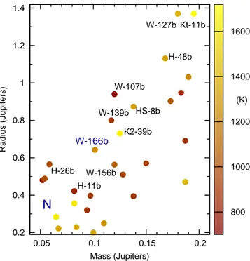
With a mass of 1.9 Neptunes, WASP-166b is the

lowest-mass planet yet discovered by the WASP survey. It also has

a bloated radius of 0.63 ± 0.03 R

. The “super-Neptune”

region of the mass–radius diagram for known, short-period

transiting exoplanets is plotted in Fig. 9, showing that

WASP-166b is near the upper size bound for a planet of its

mass. The empirically observed upper bound (from

WASP-127b to WASP-107b to HAT-P-26b) is falling rapidly in this

mass range, which may be telling us about radius-inflation

mechanisms and the ability of a lower-mass planet to hold

onto its envelope under the effects of irradiation.

For example,

Mazeh et al.

(

2016

) have shown that there

is a “Neptune desert” at short orbital periods, with almost

no hot-Neptune planets at periods < 5 d and fewer at periods

<

10 d, when compared to abundant hot Jupiters and

super-Earths (see also

Thorngren & Fortney 2018

on the lack of

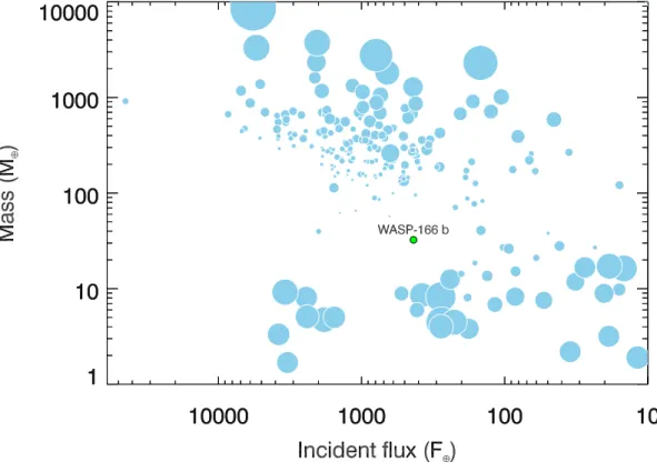
inflated sub-Saturns). To illustrate the “Neptune” or

“sub-Jovian desert” we highlight the location of WASP-166b on

a plot of planet mass against insolation (Fig. 10).

0.2 0.4 0.6 0.8 1 1.2 1.4 0.05 0.1 0.15 0.2 Radius (Jupiters) Mass (Jupiters)

N

W-166b

Figure 9.Masses and radii of transiting “hot” super-Neptune planets (with orbital periods < 10 d). The symbols are coloured according to the planet’s equilibrium temperature. The labelled planets are WASP-107b (Anderson et al. 2017), WASP-127b

(Lam et al. 2017), WASP-139b (Hellier et al. 2017), WASP-156b

(Demangeon et al. 2018), HAT-P-11b (Bakos et al. 2010),

HAT-P-26b (Hartman et al. 2011), HAT-P-48b (Bakos et al. 2016), HATS-8b (Bayliss et al. 2015), KELT-11b (Pepper et al. 2017) and K2-39b (Van Eylen et al. 2016;Petigura et al. 2017). The lo-cation of Neptune is marked with an N.

The desert is likely the result of photo-irradiation

of inwardly migrating planets (e.g.

Sestovic et al. 2018

;

Owen & Lai 2018

;

Szab´

o & K´

alm´

an 2019

). Jupiter-mass

planets are able to resist photo-evaporation, and continue

to migrate inwards by tidal orbital decay, whereas a

low-surface-gravity Neptune such as WASP-166b could not. A

hot Neptune could instead be captured into a short-period

orbit from a high-eccentricity-migration pathway, and so,

being new to its orbit, would not have undergone the

photo-evaporation that would have occurred had it migrated there

by the slower process of orbital decay. However, such

cap-ture only occurs for a narrow range of parameter space

(

Owen & Lai 2018

), and so such systems would be rare.

With a period of 5.4 d and orbiting an F star,

WASP-166b has a relatively high irradiation of 6 × 10

_{W m}

(440 times Earth’s insolation) for such a low-surface-gravity

planet. Thus it appears to be a rare object, with a radius

bloated by irradiation, on the boundary of the Neptune

desert.

The Rossiter–McLaughlin observations show that the

orbit is aligned (λ = 3 ± 5 degrees). This is consistent

with it being on a lengthy inwardly migration, during which

it has become bloated owing to irradiation. However,

re-cent capture from high-ecre-centricity pathways can also

pro-duce aligned orbits, so this is not conclusive. Relatively

few of the super-Neptune planets in Fig. 9 have had

obliq-uity angles measured, though those that have –

HAT-Figure 10. Exoplanet mass versus incident flux, showing the location of WASP-166b in the “sub-Jovian desert”. The symbol area is proportional to the bulk density of the planet. We include only planets with host stars brighter than V = 12. Data are from http://exoplanets.org/

P-11b (

Bakos et al. 2010

;

Winn et al. 2010

), WASP-107b

(

Anderson et al. 2017

;

Dai & Winn 2017

;

Moˇcnik et al.

2017

) and GJ 436b (

Gillon et al. 2007

;

Bourrier et al. 2018

)

– are all known to be misaligned.

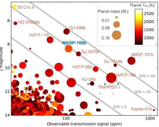
The bloated nature of WASP-166b combines with a

bright host star of V = 9.36 to make it a prime target

for atmospheric characterisation. Indeed, recent

observa-tions of irradiated low-surface-gravity planets show

indi-cations of photo-evaporating atmospheres (e.g.

Spake et al.

2018

;

Mansfield et al. 2018

). The expected signal for a

trans-mission spectrum depends on the atmospheric scale height,

transit depth, and host-star magnitude (e.g. equation 36 of

Winn 2010

). In Fig. 11 we compare the signal expected for

WASP-166b with other low-mass planets (M < 0.2 M

).

This shows that WASP-166b is likely to be among the best

targets for such studies, though this may be more difficult if

the star is indeed magnetically active, as indicated by

cor-related deviations in the RV data. We suggest that

WASP-166b is potentially a prime target for the James Webb Space

Telescope, and that it should first be observed with HST in

order to assess the cloudiness of its atmosphere.

ACKNOWLEDGEMENTS

WASP-South is hosted by the South African

Astronomi-cal Observatory and we are grateful for their ongoing

sup-port and assistance. Funding for WASP came from

consor-tium universities and from the UK’s Science and

Technol-ogy Facilities Council (STFC). ACC acknowledges support

from STFC consolidated grant number ST/R000824/1. The

Euler Swiss telescope is supported by the Swiss National

Science Foundation. The HARPS data result from

observa-tions made at ESO 3.6 m telescope at the La Silla

Obser-vatory under ESO programmes 097.C-0434 and 098.C-0304.

TRAPPIST-South is funded by the Belgian Fund for

Scien-tific Research (Fond National de la Recherche Scientifique,

FNRS) under the grant FRFC 2.5.594.09.F, with the

partic-ipation of the Swiss National Science Fundation (SNF). The

research leading to these results has received funding from

the ARC grant for Concerted Research Actions, financed

by the Wallonia-Brussels Federation. M.G. and E.J. are

Se-nior Research Associates at the FNRS-F.R.S. L.D.

acknowl-edges support from a Gruber Foundation Fellowship. This

project has received funding from the European Research

Council (ERC) under the European Unions Horizon 2020

research and innovation programme (project Four Aces;

grant agreement No 724427). This work has been carried

out in the frame of the National Centre for Competence in

Research PlanetS supported by the Swiss National Science

Foundation (SNSF). This paper includes data collected with

the TESS mission, obtained from the MAST data archive at

the Space Telescope Science Institute (STScI). Funding for

!! "

#

#

#

$ %

&

'(

) (

Figure 11.An illustration of prime low-mass planets (< 0.2 MJup) for atmospheric characterisation, based on the scale height of the atmosphere, the transit depth, and the host-star brightness.

the TESS mission is provided by the NASA Explorer

Pro-gram. We thank the many people involved in the creation of

TESS data. We acknowledge use of data from the European

Space Agency (ESA) mission Gaia, as processed by the Gaia

Data Processing and Analysis Consortium (DPAC).

REFERENCES

Anderson D. R., et al., 2017,A&A,604, A110

Bakos G. ´A., et al., 2010,ApJ,710, 1724

Bakos G. ´A., et al., 2016, preprint, (arXiv:1606.04556₎

Bayliss D., et al., 2015,AJ,150, 49

Blackwell D. E., Shallis M. J., 1977,MNRAS,180, 177

Bourrier V., et al., 2018,Nature,553, 477

Chen G., et al., 2018,A&A,616, A145

Claret A., 2000, A&A,363, 1081

Collier Cameron A., et al., 2007,MNRAS,375, 951

Dai F., Winn J. N., 2017,AJ,153, 205

Demangeon O. D. S., et al., 2018,A&A,610, A63

Doyle A. P., et al., 2013,MNRAS,428, 3164

Doyle A. P., Davies G. R., Smalley B., Chaplin W. J., Elsworth Y., 2014,MNRAS,444, 3592

Gaia Collaboration et al., 2018,A&A,616, A1

Gillon M., et al., 2007,A&A,472, L13

Gillon M., et al., 2013,A&A,552, A82

Hartman J. D., et al., 2011,ApJ,728, 138

Haywood R. D., et al., 2014,MNRAS,443, 2517

Hellier C., et al., 2017,MNRAS,465, 3693

Hellier C., et al., 2018,MNRAS,

Hirano T., Suto Y., Winn J. N., Taruya A., Narita N., Albrecht S., Sato B., 2011,ApJ,742, 69

Kreidberg L., Line M. R., Thorngren D., Morley C. V., Stevenson K. B., 2018,ApJ,858, L6

Lam K. W. F., et al., 2017,A&A,599, A3

Lendl M., et al., 2012,A&A,544, A72

Mansfield M., et al., 2018,ApJ,868, L34

Maxted P. F. L., et al., 2011,PASP,123, 547

Maxted P. F. L., Serenelli A. M., Southworth J., 2015, A&A,

575, A36

Mazeh T., Holczer T., Faigler S., 2016,A&A,589, A75

Milbourne T. W., et al., 2019,ApJ,874, 107

Moˇcnik T., Hellier C., Anderson D. R., Clark B. J. M., South-worth J., 2017,MNRAS,469, 1622

Owen J. E., Lai D., 2018,MNRAS,479, 5012

Palle E., et al., 2017,A&A,602, L15

Pepper J., et al., 2017,AJ,153, 215

Petigura E. A., et al., 2017,AJ,153, 142

Pollacco D. L., et al., 2006,PASP,118, 1407

Ricker G. R., et al., 2016, in Space Telescopes and Instrumenta-tion 2016: Optical, Infrared, and Millimeter Wave. p. 99042B,

doi:10.1117/12.2232071

Rickman E. L., et al., 2019, arXiv e-prints,

Sestovic M., Demory B.-O., Queloz D., 2018,A&A,616, A76

Spake J. J., et al., 2018,Nature,557, 68

Stassun K. G., Torres G., 2018,ApJ,862, 61

Szab´o G. M., K´alm´an S., 2019, arXiv e-prints, Temple L. Y., et al., 2018,MNRAS,480, 5307

Thorngren D. P., Fortney J. J., 2018,AJ,155, 214

Triaud A. H. M. J., et al., 2013,A&A,551, A80

Udry S., et al., 2019,A&A,622, A37

Van Eylen V., et al., 2016,AJ,152, 143

Winn J. N., 2010, preprint, (arXiv:1001.2010) Winn J. N., et al., 2010,ApJ,723, L223

This paper has been typeset from a TEX/LA_{TEX file prepared by} the author.

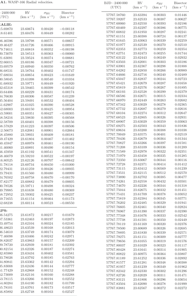
Table A1.WASP-166 Radial velocities. BJD – 2400 000 RV σRV Bisector (UTC) (km s−1_{) (km s}−1_{) (km s}−1₎ CORALIE: 56715.69870 23.60674 0.00420 −0.00118 56718.61401 23.60476 0.00449 0.00282 57186.46596 23.59798 0.00571 0.00657 57189.46427 23.61726 0.00466 0.00915 57379.74611 23.60818 0.00352 −0.00198 57420.73070 23.58513 0.00363 −0.00060 57421.63091 23.59524 0.00374 0.00681 57422.66015 23.60186 0.00347 −0.00721 57423.69579 23.60940 0.00350 0.00762 57426.68531 23.58764 0.00402 0.01747 57427.68034 23.60654 0.00423 −0.01649 57430.58045 23.61098 0.00540 0.01034 57431.68932 23.59771 0.00449 −0.01920 57432.65318 23.59465 0.00399 0.00542 57433.64406 23.60229 0.00431 0.00174 57434.76630 23.60306 0.00587 0.01239 57435.56404 23.59491 0.00532 0.00404 57451.62907 23.61025 0.00390 0.00528 57452.68003 23.60150 0.00425 0.00954 57453.59001 23.60351 0.00427 −0.00305 57458.58216 23.59830 0.00395 0.00568 57462.58709 23.60401 0.00398 0.00156 57488.57829 23.61223 0.00397 0.00506 57512.56673 23.62081 0.00901 0.02664 57558.45880 23.59931 0.00409 0.00181 57559.47429 23.61804 0.00467 0.01462 57560.45947 23.60978 0.00461 −0.00190 57561.46060 23.60891 0.00490 0.00154 57566.45959 23.61192 0.00541 0.01347 57568.46079 23.59210 0.00522 −0.00197 57716.80525 23.62126 0.00707 −0.00642 57721.78118 23.60734 0.00450 −0.01000 57722.79431 23.61259 0.00426 −0.00935 57723.79431 23.61560 0.00480 0.00999 57724.76502 23.60758 0.00470 −0.00170 57727.82177 23.60882 0.00479 0.00605 57730.78526 23.59711 0.00498 0.00324 57749.79985 23.61638 0.00480 0.00369 57758.72952 23.59302 0.00425 0.00237 57759.71655 23.61154 0.00464 0.01173 57762.68238 23.60114 0.00523 −0.00550 HARPS: 57486.54275 23.61872 0.00217 0.01679 57487.53361 23.62463 0.00197 0.02873 57523.49754 23.62104 0.00324 0.02185 57526.48623 23.63539 0.00168 0.02013 57536.54610 23.63749 0.00174 0.03079 57577.46098 23.63466 0.00242 0.02971 57728.82037 23.63863 0.00157 0.02209 57729.78720 23.62939 0.00181 0.02392 57730.82154 23.62326 0.00187 0.02274 57732.85980 23.63434 0.00402 0.03581 57733.78026 23.63792 0.00185 0.02763 57734.80841 23.63362 0.00142 0.02294 57735.83008 23.62436 0.00144 0.02777 57751.77429 23.62868 0.00152 0.02248 57752.73009 23.62116 0.00160 0.02288 57753.78115 23.63266 0.00194 0.02552 57754.80284 23.64190 0.00182 0.01799 57755.78101 23.63761 0.00173 0.03517 57756.85892 23.62748 0.00163 0.02527 BJD – 2400 000 RV σRV Bisector (UTC) (km s−1_{) (km s}−1_{) (km s}−1₎ 57767.58760 23.63394 0.00303 0.01446 57767.59207 23.62533 0.00387 0.00627 57767.60060 23.62550 0.00393 0.02186 57767.60469 23.62297 0.00386 0.00775 57767.60832 23.61950 0.00287 0.02241 57767.61151 23.60388 0.00724 0.00137 57767.61645 23.63063 0.00339 0.02259 57767.61977 23.62539 0.00270 0.02510 57767.62353 23.62773 0.00259 0.02354 57767.62751 23.62473 0.00255 0.01744 57767.63122 23.62443 0.00249 0.02932 57767.63503 23.62001 0.00303 0.03186 57767.63901 23.62367 0.00298 0.01888 57767.64282 23.62850 0.00266 0.00989 57767.64666 23.62716 0.00240 0.02489 57767.65047 23.62837 0.00244 0.02723 57767.65421 23.62679 0.00287 0.01658 57767.65819 23.62576 0.00267 0.01895 57767.66193 23.62528 0.00299 0.02379 57767.66586 23.62671 0.00315 0.02334 57767.66970 23.62449 0.00263 0.02682 57767.67342 23.63029 0.00278 0.02365 57767.67732 23.62687 0.00279 0.02616 57767.68104 23.62274 0.00312 0.02647 57767.68523 23.62805 0.00326 0.02931 57767.68907 23.63029 0.00359 0.03063 57767.69275 23.62503 0.00343 0.01836 57767.69634 23.63200 0.00388 0.01038 57767.70049 23.63575 0.00401 0.02519 57767.70436 23.62679 0.00364 0.01344 57767.70827 23.63266 0.00397 0.01581 57767.71208 23.63109 0.00336 0.01289 57767.71589 23.62978 0.00322 0.02351 57767.71979 23.63458 0.00335 0.01285 57767.72350 23.63067 0.00344 0.00116 57767.72728 23.62371 0.00414 0.01412 57767.73115 23.63412 0.00569 0.01239 57767.73531 23.62115 0.00512 0.02570 57767.73890 23.62702 0.00385 0.00477 57767.74261 23.62558 0.00432 0.03501 57767.74670 23.62226 0.00344 0.01318 57767.75044 23.62675 0.00332 0.01451 57767.75431 23.61709 0.00378 0.03052 57767.75819 23.62384 0.00345 0.03771 57767.76202 23.62485 0.00329 0.01941 57767.76605 23.62461 0.00340 0.02824 57767.76967 23.61390 0.00337 0.02390 57767.77348 23.61676 0.00333 0.02542 57767.77738 23.61591 0.00350 0.02449 57767.78119 23.61169 0.00320 0.02376 57767.78500 23.60689 0.00326 0.02685 57767.78895 23.61830 0.00339 0.02571 57767.79275 23.61151 0.00309 0.02777 57767.79656 23.61055 0.00319 0.01576 57767.80037 23.61029 0.00323 0.01117 57767.80428 23.61641 0.00314 0.01905 57767.80822 23.60975 0.00364 0.03807 57767.81189 23.61252 0.00336 0.02892 57767.81577 23.61281 0.00348 0.00388 57767.81957 23.61239 0.00349 0.01962 57767.82342 23.62330 0.00302 0.01296 57767.82726 23.62029 0.00311 0.01471 57767.83121 23.61806 0.00296 0.03654 57767.83504 23.62090 0.00278 0.01999 57767.83881 23.62567 0.00272 0.02272

BJD – 2400 000 RV σRV Bisector (UTC) (km s−1_{) (km s}−1_{) (km s}−1₎ 57767.84263 23.62769 0.00276 0.03642 57767.84646 23.62409 0.00290 0.02824 57767.85041 23.62141 0.00297 0.02191 57767.85429 23.62807 0.00285 0.02369 57767.85802 23.61976 0.00308 0.02249 57767.86187 23.62543 0.00292 0.03571 57767.86566 23.61653 0.00328 0.01006 57767.86958 23.62595 0.00320 0.03263 57767.87338 23.62471 0.00306 0.02682 57767.87724 23.62356 0.00284 0.02180 57769.80714 23.61499 0.00219 0.02590 57770.75537 23.62649 0.00281 0.02549 57816.65537 23.63019 0.00210 0.02144 57816.66032 23.62917 0.00204 0.01473 57816.67017 23.62837 0.00244 0.01715 57816.67507 23.63615 0.00262 0.01374 57816.67886 23.63392 0.00261 0.02071 57816.68266 23.63469 0.00283 0.01612 57816.68652 23.63993 0.00280 0.01991 57816.69042 23.63850 0.00285 0.02664 57816.69419 23.63915 0.00271 0.02256 57816.69791 23.63940 0.00279 0.01625 57816.70188 23.63349 0.00323 0.03297 57816.70578 23.63760 0.00310 0.02489 57816.70961 23.63197 0.00300 0.01579 57816.71334 23.63354 0.00289 0.01285 57816.71721 23.63807 0.00281 0.02084 57816.72097 23.63601 0.00292 0.02362 57816.72490 23.63239 0.00297 0.01569 57816.72856 23.63962 0.00312 0.01805 57816.73260 23.63272 0.00334 0.01253 57816.73633 23.62798 0.00317 0.02418 57816.74019 23.62777 0.00325 0.02878 57816.74404 23.62656 0.00312 0.02588 57816.74787 23.62564 0.00335 0.03502 57816.75177 23.62932 0.00324 −0.00833 57816.75556 23.62015 0.00320 0.03667 57816.75929 23.62272 0.00305 0.03631 57816.76336 23.62788 0.00344 0.02356 57816.76706 23.62189 0.00314 0.01721 57816.77082 23.61831 0.00307 0.04728 57816.77461 23.62033 0.00303 0.01428 57816.77864 23.61918 0.00347 0.03644 57816.78237 23.61925 0.00330 0.03297 57816.78610 23.61773 0.00355 0.02491 57816.79007 23.62124 0.00328 0.02607 57816.79383 23.61770 0.00337 0.02593 57816.79766 23.61668 0.00384 0.03799 57816.80145 23.60814 0.00352 0.02619 57816.80537 23.61670 0.00362 0.02351 57816.80909 23.61294 0.00376 0.02974 57816.81303 23.62676 0.00385 0.01295 57816.81682 23.62619 0.00381 0.01807 57816.82062 23.61808 0.00393 0.02724 57816.82449 23.62186 0.00398 0.03071 57816.82832 23.62480 0.00416 0.02181 57816.83212 23.62562 0.00439 0.02305 57816.83599 23.61783 0.00442 0.00742 57816.83982 23.62403 0.00471 0.02442 57816.84358 23.62622 0.00465 0.01361 57816.84738 23.61928 0.00512 −0.00844 57816.85131 23.61671 0.00493 0.02648 57816.85511 23.62293 0.00502 0.02198 57816.85898 23.61311 0.00498 0.00126 BJD – 2400 000 RV σRV Bisector (UTC) (km s−1_{) (km s}−1_{) (km s}−1₎ 57827.53425 23.62930 0.00280 0.02204 57827.53872 23.63603 0.00290 0.02670 57827.54345 23.63423 0.00285 0.02590 57827.54786 23.62957 0.00259 0.02816 57827.55227 23.63447 0.00278 0.01389 57827.55676 23.63066 0.00297 0.02514 57827.56098 23.63909 0.00305 0.02265 57827.56519 23.63729 0.00373 0.02886 57827.57028 23.64419 0.00428 0.02696 57827.57457 23.64038 0.00364 0.02522 57827.57890 23.65067 0.00382 0.02796 57827.58327 23.64449 0.00309 0.02050 57827.58769 23.64204 0.00295 0.02194 57827.59202 23.64369 0.00286 0.03653 57827.59643 23.64428 0.00285 0.02834 57827.60084 23.64191 0.00267 0.03241 57827.60533 23.63830 0.00263 0.01467 57827.60976 23.64247 0.00262 0.02718 57827.61409 23.64307 0.00264 0.01784 57827.61850 23.63863 0.00266 0.04245 57827.62295 23.63842 0.00252 0.01951 57827.62728 23.63858 0.00241 0.02096 57827.63170 23.63444 0.00238 0.02134 57827.63615 23.63524 0.00238 0.01689 57827.64056 23.63139 0.00264 0.01744 57827.64497 23.63212 0.00243 0.02347 57827.64938 23.62593 0.00239 0.02557 57827.65372 23.62390 0.00251 0.02587 57827.65821 23.62888 0.00241 0.02687 57827.66262 23.62513 0.00246 0.02387 57827.66703 23.61826 0.00244 0.03302 57827.67144 23.62351 0.00237 0.01251 57827.67526 23.60691 0.00768 −0.01366 57827.68085 23.61397 0.00330 0.02234 57827.68469 23.62346 0.00271 0.01181 57827.68917 23.61960 0.00271 0.01719 57827.69354 23.62385 0.00272 0.01891 57827.69801 23.62317 0.00337 0.03128 57827.70243 23.62472 0.00259 0.02089 57827.70685 23.62682 0.00261 0.01774 57827.71126 23.63026 0.00259 0.02072 57827.71559 23.62902 0.00272 0.00473 57827.71986 23.62284 0.00418 0.02883 57827.72448 23.63551 0.00267 0.03343 57827.72884 23.62753 0.00266 0.02473 57827.73326 23.63365 0.00270 0.02559 57827.73771 23.62836 0.00282 0.02362 57827.74242 23.62463 0.00315 0.02299 57827.74657 23.63381 0.00288 0.02348 57827.75090 23.62604 0.00292 0.01722 57827.75536 23.62729 0.00298 0.03213 57827.75977 23.62853 0.00294 0.02042 57827.76467 23.63083 0.00395 0.02306 57827.76868 23.63494 0.00308 0.04233 57827.77297 23.61858 0.00347 0.02458 57827.77742 23.63191 0.00324 0.01560 57827.78183 23.63586 0.00356 0.01705 57827.78629 23.62552 0.00359 0.02208 57827.79066 23.63287 0.00373 0.01926 57827.79507 23.62353 0.00402 0.02713 57827.79944 23.63074 0.00404 0.02189 57827.80389 23.63272 0.00406 0.01771 57827.80837 23.62434 0.00435 −0.00767 57827.81284 23.62679 0.00437 0.02713 57827.81780 23.62169 0.00599 0.03090 57827.82180 23.63132 0.00444 0.01595

BJD – 2400 000 RV σRV Bisector (UTC) (km s−1_{) (km s}−1_{) (km s}−1₎ 58198.71811 23.61212 0.00130 0.02011 58199.67572 23.61200 0.00111 0.02893 58201.64627 23.63373 0.00139 0.02105 58202.70438 23.63717 0.00119 0.01943 58203.61226 23.62522 0.00141 0.01834 58204.60885 23.61929 0.00145 0.02213 Bisector errors are twice RV errors. Lines denote an instrument upgrade, or separate through-transit sequences